Analysis of the determinants of automotive mobility behavior

HAL Id: hal-02016076

https://hal.archives-ouvertes.fr/hal-02016076

Submitted on 15 Feb 2019

HAL is a multi-disciplinary open access

archive for the deposit and dissemination of sci-entific research documents, whether they are pub-lished or not. The documents may come from teaching and research institutions in France or abroad, or from public or private research centers.

L’archive ouverte pluridisciplinaire HAL, est destinée au dépôt et à la diffusion de documents scientifiques de niveau recherche, publiés ou non, émanant des établissements d’enseignement et de recherche français ou étrangers, des laboratoires publics ou privés.

behavior

Minh Phuoc Doan, Iragaël Joly

To cite this version:

Minh Phuoc Doan, Iragaël Joly. Analysis of the determinants of automotive mobility behavior. [Rap-port de recherche] PREDIT. 2016, 70 p. �hal-02016076�

Analysis of the determinants

of automotive mobility

behavior

Rapport de recherche du programme de recherche EVOLMOB : Analyse des facteurs explicatifs de l’évolution de la mobilité urbaine –

Comparaison internationale, implications pour l’action et la modélisation

Convention de subvention : 13-MT-GO6-1-CVS-001

Septembre 2016

Minh-Phuoc DOAN

Iragaël Joly

Résumé

Ce rapport s’inscrit dans le cadre du projet de recherche EVOLMOB qui associe le LET, le GAEL (UPMF Grenoble) et l’Ecole Polytechnique de Montréal sur les évolutions récentes de mobilité.

Le but est de déterminer les facteurs les plus influents ainsi que leur évolution dans le temps grâce à l'exploitation des résultats de plusieurs enquêtes successives sur la même ville à 10 ans d'intervalle. Les données sont extraites des enquêtes ménages déplacements de Grenoble, effectuées en 2002 et 2010. L’analyse statistique du choix modal des individus est fondée sur la méthode économétrique des choix discrets, plus spécifiquement l’estimation d’un modèle logit multinomial. Son fondement dans la théorie de l’utilité aléatoire (Random Utility Theory, McFadden, 2000) permet l’estimation d’indicateurs économiques d’aide à la décision, comme les élasticités des demandes pour les modes de transport et les consentements à payer pour les attributs des modes. Les variables socio-économiques, les caractéristiques des trajets et des zones urbaines parcourues sont intégrées dans les estimations. La méthode permet d’évaluer simultanément les effets respectifs de ces variables. L’étude aborde aussi la transférabilité des résultats d’estimation entre les deux périodes d’observation des mobilités grenobloises.

Les résultats identifiés sont cohérents avec les effets attendus et identifiés dans la littérature (DeWitte et al 2013). La voiture domine les parts modales à Grenoble, mais une légère baisse est identifiée entre 2002 et 2010. Certains facteurs du choix automobile, comme le taux de motorisation ou la localisation résidentielle en zone péri-urbaine semblent voir leur effet se réduire entre les deux périodes.

Enfin, les résultats illustrent la très grande hétérogénéité des indicateurs économiques déduits des estimations, telles que les élasticités du choix modal au temps de transport ou les équivalents en temps des attributs des modes.

Avant-propos

Ce rapport est issu en très grande partie du mémoire de master 2 Sustainable Industrial Engineering réalisé

par Minh-Phuoc DOAN au sein du Laboratoire d’Economie Appliquée de Grenoble dans le cadre du projet EvolMob - Analyse des facteurs explicatifs de l’évolution de la mobilité urbaine, financé par le PREDIT sous la convention de subvention 13-MT-GO6-1-CVS-001-2013.

Analysis of the determinants of automotive mobility behavior

1. Economical literature of travel mode choice ... 5

Introduction to travel mode choice problem ... 5

1.1.1 Travel mode choice definition ... 5

1.1.2 Travel mode choice determinants ... 7

Research about travel mode choice in France ... 12

1.2.1 Paris... 13

1.2.2 Lyon ... 14

1.2.3 Grenoble ... 14

1.2.4 Conclusion ... 15

Literature conclusion ... 15

2. Method and data ... 16

Method ... 16

2.1.1 Discrete choice models ... 16

2.1.2 Model selection criteria... 22

2.1.3 Marginal effect and elasticity... 23

2.1.4 Willingness to pay and willingness to wait... 24

2.1.5 Multicollinearity ... 25

Data ... 26

2.2.1 Introduction to the French national household-trip survey ... 26

2.2.2 Data treatment ... 30

3. Results ... 32

Variable definition ... 32

Single trips ... 39

3.2.1 Model estimation ... 39

3.2.2 Mode choice evolution ... 40

Four-trip loops ... 46

3.3.1 Model estimation ... 46

4. Conclusion ... 55

5. References ... 57

6. Table of figures ... 58

Introduction:

After a continuous increase of car use in most of the metropolitans of the OECD (Organization for Economic Co-operation and Development), we witness a reversal trend in many countries with the decrease of the car use according to measured indicators and the cities. However, due to the economic crisis, the public authority doesn’t have enough financial resources to ensure the development of all the sectors of the transport network. Therefore, it’s essential to clearly understand the determinant factors of mobility behaviors and their evolution to concentrate interventions on.

Many factors have been used to explain this evolution such as population age, petrol price, congestion, travel policy, alternative modes and environmental concern.

However, which factors are the most important ones for single trips of an individual? Are their contributions to mode choice the same among different trip motives, and over time? And if we consider trips of each individual as a trip chain instead of independent single trips, will making a working trip, catching up or dropping off someone during the chain increase the probability of using car?

In order to answer these questions, we focus on two types of trips: single trips where we consider only one trip for each individual, and four-trip loops, a type of trip chains consisting of four trips in a chain and the first trip is leaving from home and the last trip is going back home. For single trips, we analyze the three common motives: home-work, home-shopping and home-leisure. For four-trip loops, we focus on three levels of complexity of trip chains (low-complexity, moderate-complexity, and high-complexity)

The studied data is based on two local household-trip surveys (realized in 2002 and 2010) in Grenoble, a medium city in France – an OECD country. Each survey is a part of the French national household-trip surveys (EMD) that have been carried out regularly in many French cities since 1976.

The most usual discrete choice model, multinomial Logit, will be used to give estimations based on commonly studied socio-economic variables: socio-demographic (gender, age, occupation, education, car availability, household size, number of women, number of men, number of cars of household) and trip characteristics (trip motive, travel time, departure time, origin zone and destination zone of trips).

From the obtained results, we hope to be able to identify and quantify the contribution of each explanatory factor to the evolution of the mode choice behaviors in Grenoble between 2002 and 2010. Thus, propose authorities of the city solutions to change the mobility behaviors that can help decrease the car use and promote the use of other eco-friendly modes like public transport, bike and walking.

In the first section, we review the literature of travel mode choice to see common approaches to this problem. In the second section, we introduce the research methods that allow to give estimations and to calculate the indicators of the evolution, and then the studied data used for estimations. The results will be presented in the third section divided into three sub-sections: variable definitions, results for single trips, and results for four-trip loops. Finally, the conclusion, recommendation, and future directions will be proposed in the last section.

1. Economical literature of travel mode choice

Introduction to travel mode choice problem

1.1.1 Travel mode choice definition

Every day, people spend a lot of time moving from one place to another place with many different trip motives such as working, studying and shopping. There are many transport modes serving this mobility demand like the car, the public transport, and the bicycle.

Choosing one of available travel modes (also called travel mode choice) is a very complex process, depending on objective and subjective, conscious and unconscious factors. The below figure describes the current view of the theory of choice (McFadden, D., 2000) that has been commonly applied to travel mode choice.

Fig. 1: The choice process (McFadden, D., 2000)

The model shows that the choice process is a decision-making process based on perceptions and beliefs built by available information and memory from past experiences, influenced by motivation, affect, attitudes and preferences.

Perception is the state of being or process of becoming aware of something through the senses. Motivation is related to the willingness to do something toward the perceived goals. Affect refers to the emotional state of the decision-maker. Attitude is a way of thinking or feeling about entities with favor or disfavor. Preference is a comparative judgment between entities.

In fig.1, the context of the current decision is based on available information, experience, and memory in the past. As a loop, the result of this choice will influence the decision-making in the future. The heavy arrows of the model correspond to the economists’ classic model (rational model) where individuals collect information on alternatives, then convert this information into quantitative perceived attributes and aggregate them into a one-dimensional utility function, which is then maximized. The light arrows coincide with the psychological factors that influence the decision-making process. Both economist’s model and psychologist’s models use the same concepts: perception, process, and preferences but have different views on how they are linked together.

Based on the model of the choice process, many different approaches to travel mode choice have been considered. De Witte, A. et al., 2013, summarized current approaches of the travel mode choice problem consisting of rational, socio-geographical, socio-psychological and multi-disciplinary approaches.

• The rational approach assumes that travelers make their decision in mode choice based on the utility maximization (minimizing travel cost and travel time). This microeconomic approach deals with all type of available information of alternatives, individuals behave perfectly rational, they just make a decision based on the objective and rational

components.

• Socio-geographical approach: in comparison to the first approach, this approach adds spatial factors into the decision-making process with the assumption that people travel not only for the sake of it but also to do activities distributed in space. So, the activity schedule of individual or household plays an important role in this approach.

• The socio-psychological approach focuses on the subjective components, especially individuals’ attitudes. Thence, intentions and habits are key elements of this approach. • The disciplinary approach is most used nowadays giving the researchers a

multi-discipline view to deal with the travel mode choice problem. This approach is the combination of all previous approaches, considering four different factor groups: socio-demographic (age, gender, education, income etc.), socio-geographical (density, diversity, parking, frequency of public transport etc.), journey characteristics (travel motive, distance, travel time, travel cost etc.) and social-psychological (experiences, familiarity, lifestyle, habit etc.).

Quantitative studies based on these variables been developed through many stages since the first model of Warner, S., 1962. Researchers try to use mathematical formulas to model the travelers’ behaviors from the data of surveys, thence, use these models to predict their future behaviors.

1.1.2 Travel mode choice determinants

A mathematical model of travel mode choice problem usually consists of one or several explained variables (also called dependent variables) and many explanatory variables (also called independent variables). Each independent variable has different influencing proportion on the dependent variables. The aim of the modeling is to quantify the contribution of each independent variable on the dependent one. The most important explanatory variables are usually called determinants. The determinants are different from each city, each country and each research’s objective De Witte, A. et al., 2013, using meta-analysis method, based on 76 published papers, presented the most commonly studied determinants in travel mode choice and then explained the importance of each determinant through the statistics of the percentage of papers in which the determinant was studied out of the number of reviewed papers and the percentage of papers in which the determinant is found to be significant out of total number of papers studying about this determinant (see Fig. 2).

Fig. 2: Statistics of frequently studied determinants in travel mode choice (De Witte, A. et al., 2013)

In her research, De Witte categorized the determinants into 4 groups according to the multi-disciplinary approach (socio-demographic, spatial, journey characteristic and socio-psychological determinants) that we presented above, and then, she summarized the studies for each determinant. Below is our summary of her article:

SOCIO-DEMOGRAPHIC

Socio-demographic determinants consist of age, gender, education, employment, income, household composition and car availability.

Age

Two different conclusions were found in De Witte’s paper: First, the physical ability to travel decreases when people become older and so, the older people are, the more public transport they use. Second, based on several other papers, he found that car use increases together with age. Gender

In term of gender, De Witte found two different views: The first one showed that men are more likely to use the car while women are likely to use the public transport. The second one revealed that women are more likely to use cars that are convenient for them with the home-work trips. Education

Education is found to be correlated with employment and income. High educated people have higher incomes than low educated people. Therefore, they are more likely to use cars. However, several other papers showed the opposite that higher educated people use public transport means more than cars.

Employment

Employment has a direct connection with income and car ownership. Full-time workers tend to use more public transport while part-time workers are likely to use cars for traveling. Besides, employed people are more likely to use cars while unemployed people are likely to use the public transport.

Income

Income has a positive influence in car use and negative influence in public transport use. People with high income tend to travel by car instead of public transport while people with low income are highly influenced by the transport cost. However, in several studies, income was found not to influence on professional trips.

The household composition has very big impact on a number of cars per household. Increasing the number of members in a household especially number of children is likely corresponding to an increase of car use and a decrease of public transport use.

Car availability

Increasing the motorization rate (number of cars per household) reduces the competition for car use among household members and therefore, increases the car use, decreases the use of shared-ride and public transport means. Households without car likely depend on public transport and non-motorized means. Besides, the odds of train use in comparison to car use decreases 52% corresponding to one unit increase in a number of cars, and decreases 96% if the household can use the company’s car.

SPATIAL

Spatial determinants characterize transportation networks and services consisting of density, diversity, proximity to infrastructures and services, the frequency of public transport and parking. Density

Density is the ratio between a number of inhabitants and living area. It has a very strong negative influence in the average trip distance, thence, stimulates the public transport, bike and walking. Besides, public transport has been found to have higher service quality urban areas (high density) than in rural areas (low density) which impact directly travel time and travel cost and as a result promotes the use of public transport.

Diversity

Diversity is related to the land-use mix such as residence, institution, industry, commerce etc. Land-use mixtures tend to reduce the car use and increase public transport use.

Proximity to transport infrastructures and services

Proximity to transport infrastructures and services is related to the accessibility to road networks and public transport infrastructure. This determinant has direct connections to density and diversity at both the origin and destination. Accessibility to the public transport station increases its use, especially at the destination. Besides, car use increases together with the increase of road availability.

Frequency of public transport

High frequency of public transport creates a comparative advantage with regard to other modes. As a result promotes public transport use. In contrary, poor public transport services lead to lower public transport use.

Parking is a quite important determinant. In most of the case, people tend to use cars when they are assured to have a parking space, especially free one. Decreasing the number of parking lots in the city is likely to decrease the car use and increase the public transport use.

TRIP CHARACTERISTIC:

Trip characteristic determinants consist of travel motive, travel distance, travel time, travel cost, departure time, trip chaining, weather condition, information and interchange.

Travel motive

Travel motives can be divided into three main types: commuting, professional and leisure. Commuting trips, especially school trips, share higher use of public transport than other motives while professional trips have the highest share of car use. With the leisure motives, the picking-up/ dropping-off, shopping, and long trips are likely to be made by car more than the others. Travel distance

People tend to choose faster transport means for longer distance trips. In Brussels, the car is the most used mode for the short trip (less than 30 km). For longer distance, public transport is likely to be used for commuting trips. For access mode of multimodal trips, walking was dominant for distances up to 1.2 km, biking for distances between 1.2 and 3.7 km and public transport for distances being longer than 3.7 km. With exit mode, walking for distances up to 2.2 km and public transport for longer distances.

Travel time

Travel time depends on the travel motive (working, studying, leisure etc.). People tend to use public transport for longer travel time trips and car for shorter travel time trips. Increasing the travel time of public transport will decrease its demand. Besides, people don’t consider only in-vehicle travel time but also out-of-in-vehicle travel time including walking time, waiting time and parking time.

Travel cost

Consumers are quite sensitive to changes in price, especially with public transport. If a public transport pass is owned, its use will increase. The increase in public transport fare in relation to car use expenses will decrease its use and increase car use. However, a small number of car drivers hope to switch to transport public when its fare goes down.

Departure time

During the off-peak hours, due to low congestion, cars are more attractive than public transport. Besides, departure time is related to travel motive. For working or studying trips, people must travel during peak hours. Therefore, they are more likely to choose public transport.

Trip chaining

Model choice is determined by all trips in the chain between the origin and the destination. The trip chaining is only significant for multiple-chain trips. Public transport chains are found to be more complex than car chains and so, for multiple-chain trips, they appeared to be less attractive than cars’. For trip chaining with intermediate activities between origin and destination, people tend to choose the travel means that are the most convenient for these activities. Public transports appeared to be negative in this point of view.

Weather condition

Weather rarely appeared in papers about travel mode choice. Trips made by bicycles are more likely to be shifted to other modes in winter or in bad weather. Besides, 20% of the main employees change their mode of travel in summer.

Information

Easy-access information is found to be important for public transport mode. Information about congestion and delays can help to reduce users’ stress and therefore, increases the transport mode use.

Interchange

Interchange is related to how transport networks are designed to complement each other. Bad transport public connections will increase the car use.

SOCIO-PSYCHOLOGICAL:

Socio-psychological determinants are composed of experiences, familiarity, lifestyle, habits and perception

Experiences

Past experiences evidently determine present travel mode choices. People with high experiences of road network tend to use private transport mode to go to work.

Familiarity

Familiarity is related to experiencing to different modes of transport. It appeared that using public transport in the past gives people skills and confidence to use it again in the future. Higher familiarity to a transport system reduces the barriers to switch to alternative modes. Besides, familiarity is related to occupation, students were highly influenced by familiarity with public transport system.

Lifestyle is the way of living of a person. It’s directly related to education and occupation. Individual lifestyle is a very important factor in travel mode choice.

Habit

People with a strong habit of a transport mean tend to be passive in exploring other alternatives than people with a weak habit.

Perception

Preferences are based on attitudes and perceptions. The slowness of public transport is not just about travel time but also about how people experience it. The cost of car use is often underestimated compared to the price of public transport.

De Witte’s article gave an introduction to the most commonly studied determinants in the world based on 76 international articles. However, travel mode choice in each geographical area is not the same. In order to have a better view about determinants of travel mode choice in Grenoble, our studied city, we will take a look at several studies about this problem in France, especially in the two biggest French cities (Paris and Lyon) and then we look at previous studies in Grenoble.

Research about travel mode choice in France

The car is one of the most important transport modes in France. According to Roux, S. et al, 2010, based on the French National Travel Survey, car ownership of household increased significantly from 50% in 1966 to 80% in 2007. The average number of cars per household has increased strongly with the rate of 0.6 for a one-person household and 1.7 for households with 3 people or more.

Fig. 3: Average number of cars per household by household size at different period (source: Roux, S. et al, 2010)

The increase of car use over year has caused many problems for French cities, especially congestion and pollution. According to the INRIX France Traffic Scorecard, the congestion has caused major impacts on the French economy and environment. Besides, through 25 worst bottlenecks of the country, drivers spend on average 70 hours a week. Paris is the most congested city in Europe, followed by London, UK. The top congested cities in France are Paris, Lyon, Lille, Limoges, Marseille, and Grenoble.

1.2.1 Paris

Paris is the largest and also the most congested city in France. Between 1998 and 2020, Paris population is forecasted to increase 16%. Many studies to quantify the contribution of factors in the increase of car use have been carried out.

Papon, F., 2002 carried out a research about the forecast of travel by car and public transport in Paris by 2020. The research based on the trend observed since 1980 taking into account termed structure factors (age, residential zone, car ownership), explanatory variables (income, transport price, transport supply) and traffic variables (network congestion, trip frequency, travel time, aggregate quality indicators). The result indicated that there will have totally an increase of 25% in public transport use and 50% in car use in 2020 compared to 1998. The structural variables cause 8% increase for public transport use and 40% for car use. The influence of economic variables (income, transport supply, transport price) is 16% increase in public transport use and 7% increase for car use.

De Lapparent, M., 2003, used the discrete choice model to analyze traveler’s demand for transport alternatives. In his research, he considered wide range of variables: individual characteristics, tastes and psychologies, transport market attributes and income effect. The research showed that travel cost and travel time are significant in any considered model, driving license, private mobility, and transport network structure are decisive in transport mode choice. The presence of income effect impacts on travel mode choice indirectly through the increase of the average value of time.

Another article of De Lapparent, M., 2005, studied about travel mode choice of home-work trips in the Ile-de-France region. The research considered influences of socio-demographic variables (age, sex, income, residential zone) and trip characteristic variables (travel time, travel cost, departure time) on the choice of two alternatives (private motorized vehicle and public transport). The conditional Logit model revealed the importance of travel time, travel cost, departure time and income with the travel mode choice.

De Palma, A., and C. Fontan, 2001 studied travel choice and value of time based on the data of the travel survey of Ile de France region, 1997. The research studied the influence of variables (age, sex, income, residential place and working place) to the value of time over two travel modes (public transport and private car) by using Logit model with income effect. The final results showed the influence of considered variables on the value of time of two transport modes.

1.2.2 Lyon

Although Lyon is the second biggest city in France, there are currently not a lot of published studies about travel mode choice in this city.

Bonnel, P., 2000, studied trends in public transport and car use in Lyon, showed that there was an evolution in public transport use of the city with an increase of 35% (double of metro use) in 1995 compared to 1986. However, the market share of public transport (profit) has decreased from 23.5% to 20.6% while car’s increased 25% in the same period. This trend is forecasted to continue in next ten years with the decrease of 10% of public transport.

Pronello, C., and V. Rappazzo, 2014, aiming to test the traveler behaviors to the congestion pricing policy, showed that people who use cars for daily working trips have a higher willingness to pay than ones who use cars for leisure trips. Researcher divided participants into 6 groups corresponding to the acceptance level from most positive to most negative: supporter, positive attitude, open-minded taking into account pros and con, negative attitude, strong opponents, and fierce opponents. Each type of participant have a different point of view about congestion charging but have a common view that a high rate of charging will definitely reduce the number of car use.

1.2.3 Grenoble

Grenoble is the second largest urban in the Rhone-Alpes region, 11th largest by population in France (INSEE French national statistical office, 2013). However, the number of studies about the travel mode choice in this city are quite limited.

Bonnel, P., 1995, considered the changes in behaviors of residents through activity-based travel analysis. The research was carried out in 1987 when the first tram line was opened and a year later (1988), based on the surveys of 478 people (416 people agreed to be surveyed again in 1988) who live within half a mile from tram stops or on a bus route that take them directly to the tram line. The research focused on three modes of transport: foot, car and public transport (other modes share: less than 5%), three variables: sex (man or woman), professional activity (working or non-working) and car availability (available or not). The results showed that there were not a lot of differences between activity-based travel in 1987 and in 1988 except for the non-working woman with cars (up to 17.5% in 1988 from 7.5% in 1987). He explained that the reason for this difference is not due to the establishment of new tram line but the evolution of the social and economic environment.

The research carried out by Gandit, M., 2009, analyzed the influence of socio-demographic, structural and psychological factors on the choice of three travel modes: mass transit, mixed mode or private car. Researched revealed that socio-demographic factors like gender, age, the number of children, income had no effect on travel mode choice, structural and psychological factors like attitude, norms, facilitating conditions, habit had significant impacts on mode choice, especially habit ( major determinant). The research also considered the change in residents’ behaviors when a new tram line was built in Grenoble. The result indicated that building alternative means created positive views on non-car vehicles and if this image was promoted to impact on residents’ perception, public transport use would be likely to increase. Besides, the monetary policy (fare reduction) is also a good tool to stimulate public transport use and demote car use.

A recent research implemented by Hansen, R., 2008, analyzes the daily mobility in the Grenoble metropolitan region. The research based on data from 39 completed travel diaries from 22 households, considered the influence of three factors (gender, the day of week and work status) on travel mode choice. The results showed that work status was a significant explanatory variable while the others can’t be used to explain the behavior changes.

1.2.4 Conclusion

Through recent studies about travel mode choice in France, we find out that:

Age, sex, occupation, car ownership, driving license, income, number of children, residential zone, working zone are the most often studied socio-demographic variables. Among them, car ownership, income, occupation, driving license and residential zones are found to be significant in most of the cases.

For trip-characteristic variables, travel time, travel cost, departure time, a number of connections, trip frequency and the day of week appeared quite often. Among these variables, travel time, travel cost, departure time and trip frequency are found to be very important.

Spatial and socio-psychological variables are not studied regularly. However, socio-psychological variables (attitudes, norms, habits) appeared to be quite important each time they were studied. The results of studies in France are quite similar to De Witte’s research. However, we found new variables that didn’t appear in De Witte’s research, consisting of driving license, residential zone and working zone. We will also consider these variables in our research.

Literature conclusion

In our research, we focus on two types of variables:

First, the most important variables according to De Witte, A. et al., 2013 and to the articles about travel mode choice in France, that are: income, occupation, car ownership, car availability, driving license, travel time, travel cost, departure time, trip frequency and residential zone.

Second, classical variables that are commonly studied in the literature of travel mode choice: age, sex, education, the number of children, household size, travel motive, distance, proximity to infrastructure, working zone, origin zone, destination zone, and trip chaining.

However, depending on availability and quality of surveyed data and the interdependency of variables, proper variables will be then selected for our analysis.

In the next section, we will discuss methods used to give the estimations of travel mode choice based on these variables and then, the real databases obtaining from the local surveys in Grenoble in 2002 and in 2010. Both of them will allow us to select the good-quality variables for our models.

2. Method and data

Method

2.1.1 Discrete choice models

Choosing one of available travel means is a type of discrete choice where alternatives are a car, public transport, non-motorized and other modes.

Depending on a number of possible alternatives and their type of data, we obtain different models: binomial model (two alternatives), ordinal model (ordinal alternatives) and multinomial model (at least three alternatives). For the travel mode choice problem, the alternatives are unordered, so only the two first models (binomial and multinomial models) are considered.

The discrete choice is usually built on the platform of decision maker's preferences (assumption of utility maximization):

A decision-maker labeled n, has to choose one among J alternatives. The utility function of the decision-maker n obtained from the information of alternative j, labeled Unj, j=1..J

The utility function can be divided into two parts: observed utility Vnj (depending on attributes of

the decision-maker n and the alternative j) and unobserved utility

ε

Unj= Vnj+

ε

Depending on the distribution of unobserved utility, we obtain different discrete choice models. Most common used models are Probit and Logit. The Probit model uses the normal distribution function while the Logit model uses the Gumbel distribution function (also called Type I extreme value).

There is not much difference between these two models, each model has its advantages and disadvantages. However, in scientific papers about travel mode choice, Logit is the most widely used model, the share of Probit is quite small. The reason is not about the accuracy of the model but about its economical aspect. McFadden, who obtained the Nobel Prize for his contribution to consumer choice behavior analysis, developed the Logit model theory with a direct connection to the consumer theory. It permits to link unobserved preference heterogeneity to a fully consistent description of the distribution of demands (McFadden, D., 1974).

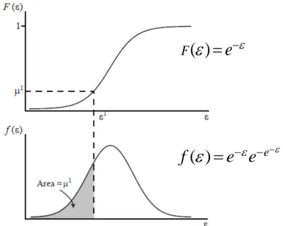
The Logit model is obtained by the assumption that each

ε

cumulative distribution function and the density distribution function as follows:

Fig. 4: Cumulative (above) and density (below) distribution functions of Logit model

The Logit model can be divided into multinomial Logit model, generalized extreme value (GEV) model and mixed Logit model (also called random parameters Logit model).

The multinomial Logit model (also called conditional Logit model) is the standard Logit model that can be derived as follows:

The probability that the decision-maker n choose the alternative i:

Pr

(

,

) Pr

(

,

)

ni ni nj ni ni nj nj

P

=

ob U

>

U

∀ ≠ =

i

j

ob V

+

ε

>

V

+

ε

∀ ≠

i

j

Combining with the assumption that

ε

(

)

nj

f

ε

=

e

e

, we obtain the Logit choice probability:

ni nj V ni V j

e

P

e

=

∑

( )

f

ε

=

e e

( )

ε

=

e

The observed utility is usually used under the linear form:

V

β

x

of observed variables. So, the Logit choice probability becomes:

xni xnj ni j

e

P

e

=

∑

In this model, the odds ratio of any set of two alternatives doesn’t depend on the choice of other alternatives. This independent property of the multinomial Logit model comes from the initial assumption that the disturbances are independent and homoscedastic (IIA assumption).

This IIA assumption gives many advantages if it truly reflects the reality:

It permits to estimate model parameters consistently on a subset of alternatives. Exclusion of alternatives in estimation does not affect the consistency of the estimator. Therefore, it is very attractive for researchers being interested in examining choices among a subset of alternatives and not among all alternatives (Train, K., 2003).

Although this property is very useful for the estimation, it is not so attractive for studies about consumer behaviors (Greene H., 2012). If the IIA assumption is not realistic and the unobserved utility is correlated over alternatives, keeping using these models can cause significant errors on forecasting substitution patterns.

Therefore, testing this assumption has an important role in selecting which Logit model to use. The first developed test is the test on subsets of alternatives that aims to check if the ratio of probabilities between any two alternatives is the same or not when other alternatives are available in the model. The test is based on chi-squared distribution with K degrees of freedom (Hausmann, J., and D. McFadden, 1984):

2 1

( _{s f}) '[V_s V_f] ( _{s f})

χ ₌ β ₋β ₋ − β ₋β

Where, s: estimators based on the restricted subset, f: estimators based on full set of choices Vs, Vf : respective estimates of asymptotic covariance matrices.

Negative test statistics ( 2

0

χ < ) are very common, Hausmann, J., and D. McFadden, 1984 concluded that a negative result is an evidence that IIA has not been violated.

In case of failure of IIA assumption, it appears that the best advice is to go back to an early statement by McFadden, D., 1974, that the multinomial Logit models should only be used in cases where the outcome categories ‘‘can plausibly be assumed to be distinct and weighed independently in the eyes of each decision maker.’’ Similarly, Amemiya, T., 1981, suggests that the multinomial Logit model works well when the alternatives are dissimilar.

Generalized extreme value (GEV) models and mixed Logit models show great promise for models violating this IIA assumption.

In GEV model, the unobserved portions of utility for all alternatives are jointly distributed as a generalized extreme value. This distribution allows the correlations of alternatives. However, if all the correlations are zero, these GEV models become standard Logit models.

The most commonly used members of this GEV family are Nested Logit and Heteroskedastic Logit models.

The nested Logit model is used when the set of alternatives can be divided into subsets (nests). For example, a nested Logit model with 2 branches (Branch1, Branch2) and 5 choices

(c

, c

c

c

c

)

Fig. 5: A nested model with two branches and five choices (Greene, H., 2008)

For any two alternatives in the same nests (for example

c

, c

)

other alternatives. But not for two alternatives in different nests (for example

c

, c

)

ratio can be dependent on other alternatives. This means IIA assumption is held within each nest and not held between different nests.

Although the complexity of the nested model depends significantly on the number of levels, the model has been extended to three levels or higher. The reason is that it is a very flexible model and suitable to consumer choice in econometric studies.

There are problematic aspects of the nested Logit model that the estimation results depend on the way of branching. Bhat, Allenby and Ginter, developed an extension for conditional Logit model to solve this problem called heteroscedastic extreme value model (Greene, H., 2008). The model comes out with the idea that instead of capturing the correlations of alternatives, we can allow the variances of unobserved utility to be different between alternatives.

The mixed Logit model, also called random parameters Logit, is a random coefficients formulation. Allowing the coefficients to vary randomly across individuals and the correlations between constant terms can help to create a general flexible model that can approximate any random utility model. Train, K., 2003 and McFadden, D. and K. Train, 2000, showed the comparative advantages of mixed Logit model and other Logit models, also between mixed Logit model and Probit model:

"It [Mixed Logit] obviates the three limitations of standard Logit by allowing for random taste variation, unrestricted substitution patterns, and correlation in unobserved factors over time." “Mixed Logit can also utilize any distribution for the random coefficients, unlike Probit which is limited to the normal distribution. It has been shown that a mixed Logit model can approximate to any degree of accuracy any true random utility model of discrete choice, given an appropriate specification of variables and distribution of coefficients."

The unconditional choice probability of mixed Logit model ( in case the utility is linear) is as follows: ' ' 1 ( ) ( ) ni nj x ni J x j f d e P e β β β β = =

∫

∑

Where

f

( )

β

' ' 1

( )

e

L

e

β

=

∑

β

Based on its formula, we can see that mixed Logit probabilities are the integral of standard Logit probabilities over a density of parameters.

The table below summarizes the advantage and disadvantage of different Logit models we presented above:

Table 13

Model Advantage Disadvantage Multinomial

Logit

- is standard and simple

- can represents systematic taste variation

- implies proportional substitution across alternatives

specification of representative utility

- can capture the dynamics of repeated choice if unobserved factors are independent over time - can be solved quickly by

computational software

- does not represent random taste variation

- is not enough flexible to capture different forms of substitution - can’t deal with unobserved factors being correlated over time - should respect IIA assumption

Nested Logit - allows to relax IIA assumption => more flexible substitution pattern (proportional in the same nest)

- used when alternatives can be partitioned into subsets

- is more complex than

Multinomial Logit => researchers need to help the routines by different algorithms

- does not represent random taste variation

- can’t deal with unobserved factors being correlated over time Heteroskedastic

Logit

- allows different variances between alternatives => accepts many different substitution patterns

- does not represent random taste variation

- can’t deal with unobserved factors are correlated over time Multinomial

Probit

- can handle random taste variation - allows any pattern of substitution - can handle problems that

unobserved factors are correlated over time

- requires normal distributions for all unobserved components of utility => inappropriate in some situations

Mixed Logit - is very flexible, can approximate any random utility model

- can solve three limitations of standard Logit

- is more difficult to be solved, requires very strong computational tools

Although Logit models have been developed for a long time, their application has only become widely popular with the appearance of strong computational sorts of software in last several decades.

Nowadays, the conditional Logit model can be solved instantly by computation tool even with a large number of alternatives and observations or non-linear elements. However, achieving and verifying the convergence of the models is still a hard issue, for example, multinomial Probit model with an unrestricted covariance structure continue to resist conventional computation (McFadden, D., 2000).

Therefore, the simulation tool is becoming practical presentation. A model where simulation methods are usually needed is the mixed Logit model that was developed by Mc Fadden in 1989, Bolduc in 1992 and Brownstone and Train, 1998 (McFadden, D., 2000).

2.1.2

Multinomial Logit model selection criteria are based on maximum likelihood method:

The probability density function for a random variable x conditioned on a set of parameters β, labeled

f x

( | )

β

1 2 1 , ,..., ( )

(

| )

( | )

|

f x x

β

f x

β

=

_∏

β

|

This function is a function of an unknown set of parameters β and collected data sample x.

The principle of maximum likelihood is that the model parameters will be estimated in the way that likelihood function (model probability) obtains the maximum value. This means that obtained set of parameters will make this collected data sample most probable.

Besides, a multinomial Logit model can be also selected based on indicators of the goodness of fit such as Akaike information criterion (AIC) and Bayesian information criterion (BIC)

Akaike information criterion (AIC) and Bayesian information criterion (BIC) are two model selection methods allowing us to penalize the loss of degrees of freedom when new variables are added to the models:

2 2 ln

AIC= k− L

ln 2 ln

BIC =k n− L

Where k: number of parameters, n: number of observations, L: maximum value of the likelihood function

In these criterions, the models with smaller values of AIC or BIC are preferred.

The BIC model has a higher penalty for the loss of degrees of freedom than the AIC model. However, each model has advantages over the other one.

2.1.3 Marginal effect and elasticity

Marginal effect

Direct marginal effect is defined as the change of the probability Pni of choosing alternative i of

individual n given by a change of an observed variable, Xni , entering the observed utility of that

alternative while keeping the observed utilities of other alternatives as constants (Train, K., 2003)

(1 ) ni ni ni ni ni ni P V P P x x ∂ ₌∂ ₋ ∂ ∂ , where ni nj V ni V j e P e =

∑

If the observed utility is linear in xni with coefficient βx, we obtain:

(1 ) ni x ni ni ni P P P x β ∂ _{= −} ∂

This marginal effect is biggest when Pni=0.5 and becomes smaller when Pni approaches one or zero

Similarly, we can obtain cross marginal effect that is a change of the probability Pni of choosing

alternative i of individual n given by a change of an observed variable, Xnj ,of another alternative

j, entering the observed utility of the alternative while keeping the observed utilities of other alternatives as constants (Train, K., 2003)

ni ni ni nj nj ni P V P P x x ∂ _{= −}∂ ∂ ∂ , if Vni is linear, ni x ni nj nj P P P x

β

The direct elasticity of Pniwith respect to Xni is the percent change in the probability of choosing

alternative i of the individual n that is associated with the percent change of variable Xni

ni ni ni ix ni ni

P x

E

x P

∂

=

∂

(1

)

P

V

e

P

and

P

P

x

x

e

∂

∂

=

=

−

∂

∂

∑

So, ni

(1

)

V

E

x

P

x

∂

=

−

∂

If the observed utility is linear in Xni with coefficient βx,

(1

)

ni

ix x ni ni

E

=

β

x

−

P

Similarly, the cross-elasticity of Pni with respect to a variable entering alternative j:

(1

)

nj

ix x nj nj

E

= −

β

x

−

P

2.1.4 Willingness to pay and willingness to wait

Willingness to pay (WLP) expresses how much consumers value the attributes of the choices. There are two ways to estimate the willingness to pay for one attribute: using the marginal utility of income or marginal utility of cost.

WTP = Marginal Utility of Income / Marginal Utility of Attribute Or WTP = - Marginal Utility of Cost / Marginal Utility of Attribute The formulas of WTP can be derived as follows:

We consider the influence of the change of attribute Xni to the change of income INni while the

other attributes are kept as constants:

0

U

β

IN

β

X

∂

=

∂

+

∂

=

The change of utility of cost is opposite to the change of utility of income, so we obtain the negative sign for the formula of WTP if we use Marginal Utility of Cost.

Similarly, Willingness to wait (WLW) expresses how much consumers value the attributes of the choices through the time they will be willing to wait if the attributes of choices are improved. The willingness to wait can be calculated using the marginal utility of travel time.

ni X ni TT TT WTW X β β ∂ = = − ∂ 2.1.5 Multicollinearity

Multicollinearity is a data problem where the explanatory variables are too highly inter-correlated to allow precise analysis of their individual effects. If the two variables are perfectly correlated, the variance will be infinite. This causes a failure of the linear regression assumption.

However, this problem doesn’t appear so often. The most common case is when attributes are highly but not perfectly correlated. The assumptions are held but there will be severe statistical problems like small changes in the data produce wide swings in the parameter estimates, Coefficients may have very high standard errors and low significance levels even though they are jointly significant and the R2 for the regression is quite high or coefficients may have the “wrong” sign or implausible magnitudes (Greene, H., 2008).

The most common methods used to diagnostic the Multicollinearity are based on variance measurements like correlation matrix, condition number and variance inflation factors (VIF and GVIF)

The correlation matrix used to evaluate the independence between multiple variables at the same time. Most common correlation matrices are Pearson (used for continuous variables) and Spearman (used for ordinal variables). A value in the correlation matrix (off-diagonal elements) exceeding 0.9 is sometimes considered as a potential problem (Hair, F. et al., 1998).

The condition number of a matrix is the square root of the ratio of the largest to the smallest characteristic root: max min

λ

γ

λ

=

This method is suggested by Belsley, D. et al., 1980. Belsley showed that a value of condition number in excess of 20 can be a potential problem.

The Variance inflation factors quantify how much the variance is inflated. The variance inflation factor for the kth factor: 1 ₂

1 k k VIF R = − where 2 k

R _{is the R}2_{-value obtained by regressing}

the kth predictor on the remaining predictors

Values of VIFs exceeding 4 warrant further investigations, while values exceeding 10 are signs of serious multicollinearity.

The GVIF was introduced in Monette G. et al., 1992. The GVIF is important to diagnostic the multicollinearity of factors and polynomial variables where a variable require more than one coefficient. For single variables, GVIF equals to VIF. GVIF^(1/2df) where df is a degree of freedom or number of coefficients of a variable, is used to make GVIF comparable across dimensions. A value of GVIF^(1/2df) in excess of two can be a potential problem.

The multinomial appears to be a quite good choice for our estimations. Firstly, it’s a standard and most simple Logit model that can give a quite efficient estimation. Secondly, it’s well supported by computational tools allowing us to calculate marginal effect and elasticity that other Logit models can’t obtain easily. Finally, multinomial Logit selection based on maximum likelihood allows high multicollinearity among variables, thus, allow to build a large model with many variables that are limited in other Logit models.

However, we have to be caution in case of failure of IIA test. If this happens, we can keep using this model but the confidence of substitution patterns between modes can be at risk.

Data

2.2.1 Introduction to the French national household-trip survey

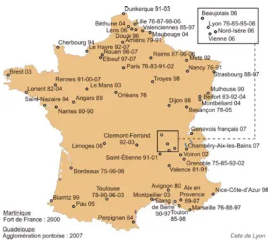
The data is based on the Household-Trip Survey in the whole French territory that has been carried out since 1976, with around 70 surveys in more than 40 French metropolitans.

Each survey is a photography of the trips made by the inhabitants of a region during a particular day of week and by all the transport modes (public transport, private car, bicycle, etc.).

The survey allows us to measure the mobility evolutions to estimate the impact of implemented actions and to adapt new travel policies. The results of the survey will support the authority to make a decision in travel policies.

Fig. 6: Maps of household-trip surveys (EMD) in France from 1976 to 2007

The survey has used a standard method defined by CERTU (Centre d’Étude et de Recherche sur les Transports et l’Urbanisme) respecting following principles:

Carried out:

- On all the trips made by people who live in the studied area on the day before the survey. - At home, face to face (during about 1h30’) by trained interviewers, from Tuesday to

Saturday

- Over a long period between 15 October and 30 April, excluding public holidays and school vacations

- On people being more than 5 years old and having a housing

- On a representative sample of households, randomly selected based on resident zone and housing file

The database consists of five subfiles:

- Household (Ménage): contains household characteristics like location, housing, the number of members and motorization.

- Person (Personnes Du Ménage): contains individual socio-demographics like age, gender, occupation, education, driving license and car availability.

- Trip (Déplacements): contains trip characteristics like travel time, departure time, travel motive and travel distance.

- Path (Trajets): contains information related to path characteristics like walking time, the number of occupants, parking place, and highway toll.

- Opinion (Opinions): made by a member of each household being more than sixteen years old, containing opinions about transport system: criteria in choosing transport modes, speed qualification of transport modes etc.

EMD Grenoble 2002 and 2010:

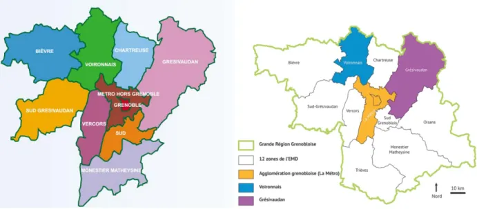
Our Grenoble 2002 database was taken from l’Enquête Ménages-Déplacements Grande Region Grenobloise 2002 (EMD Grenoble 2001-2002), carried out in an area of 254 villages with 712 000 inhabitants where 17254 individuals of 6963 households were interviewed (SMTC, “Résultats EMD 2002: Grande Région Grenobloise”).

Our Grenoble 2010 database was taken from EMD Grenoble 2009-2010 that was carried out during 18 weeks between 2009 and 2010 by 240 investigators, on 7600 households, in a large area of 354 villages with more than 800000 inhabitants. (SMTC, “Résultats EMD 2010: Grande Région Grenobloise”)

Fig. 7: Surveyed area of EMD Grenoble in 2002 (left) and in 2010 (right)

Here are some characteristics of the data from the two surveys (source: SMTC, “Résultats EMD 2002: Grande Région Grenobloise”, SMTC, “Résultats EMD 2010: Grande Région Grenobloise” and Licaj, I. et al, 2015):

Table 14

Data summary of EMD Grenoble 2002 and 2010

Variable/ Year Grenoble 2002 Grenoble 2010

SOCIO-DEMOGRAPHIC

Population age 25% less than 18 years old, 13% greater than 65 years old

Old population, 23% less than 18 years old, 17% greater than 65 years old

Profession 53% is workers and

employees

43% is active (full-time or part-time), most of jobs are in service sector

Education 25% (of > 5 years old) has education lever higher than BAC, 27% is studying at school

5% is student, 28% (of > 5 years old) has education lever higher than BAC

Driving license In general: 85% Men: 93% Women: 78%

In general: 86% Men: 92% Women: 81%

Household composition 2.41 person/household 2.25 person/household 1/3 is single

Car ownership 1.26 cars per household, 0.51 car per individual

0.58 car per individual TRIP

CHARACTERISTICS

Mode share 62% by cars

10% by Public transport 24% on foot 59% by cars (46% driving, 13% accompanied) 11% by Public transport 25% on foot

Trip purpose (motive) Working: 14% Shopping: 12% Leisure: 16%

Accompanying: 13% School and university: 12%

Working: 23% Shopping: 18% Accompanying: 16% School and university: 12%

Average number of trips per individual per day

2.2.2 Data treatment

Our research is based on two household-trip databases of Grenoble in 2002 and 2010.

The objective of the data treatments is to build a reliable, clean, and similarly-structure data frame, that is commonly implemented by R, a free and high-performing statistical analysis tool. In order to do this, we face with two different choices: First, Treating the original database by the available SAS code built by previous research groups to get the intermediate database, then building new R code to convert this database to the final one for analysis. Second, ignoring the available SAS code and building new R code to treat the original database. Using the first solution, we can take advantage of very large available SAS program and save up a lot of time. The only problem is that we have to work with both programming languages that are completely different. Luckily, the SAS programming language is quite similar to other language taught at most of the schools, understanding how it works doesn’t take us too much time. So, we decided to follow this direction. Fig.8 shows the diagram of the data treatment

Each original household-trip database consists of four sub-database files: Household file, individual file, trip file and path file. This data will be treated by two programs: SAS and R. Firstly, the SAS program imports the four files of the original database to its environment. In order to obtain an aggregated database that trip is the lowest level, the SAS module “Integrate path data into trip level” helps to integrate the data of all the paths of each trip with one another. In this process, the trip traveling mode is defined by combining traveling mode of each path of the corresponding trip.

Secondly, the integrated path data will be aggregated with the three remaining database files to create aggregated database. The database then goes through three processing steps: unit standardization, data errors detection and deletion, variables definition. The process of unit standardization converts the data units to the standard types, especially converts all the units of timing data to minute. The process of data errors detecting helps to detect common data errors (departure time is later than arrival time, travel time is negative, lack of departure time or arrival time etc.) These wrong data will be modified or deleted. After that, explanatory variables will be defined to create the intermediate database that will be treated later by R program.

The R program then imports the intermediate data into its environment. Based on research scope, inappropriate data is removed from the database:

- Individuals who didn’t make any trip during the surveyed day

- Individuals with unclear resident place or at least one unclear origin or destination zone of any trip

- Individuals who lived, worked or had at least one trip origin or destination in the external zones

Treated database allow us to remove poor-quality data or data that is not related to our scopes. From now on, the database can be used to define proper variables for our study. In the next section, final variables will be defined and then, our two models (single trip and four-trip loop) will be built to allow analysis of the evolution of travel mode choice.

3. Results

Variable definition

Our analysis focuses only on three motives of single trips (work, shopping and home-leisure) and three complexity levels of trip chains of 4-trip loops where their first trips are leaving from home and their last trips are going back home. Other motives of single trips and other trip chains of four-trip loops either occupying a very small proportion of a total number of trips/loops or appearing to be too complicated to study will be removed.

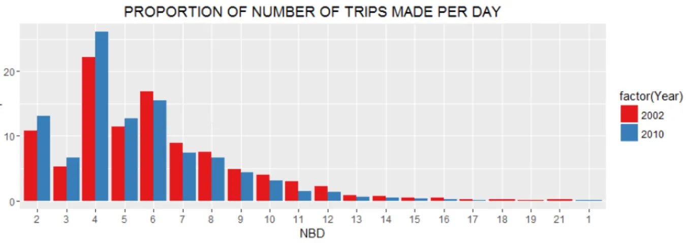
Fig. 10: Histogram of number of trips made per day in 2002 and 2010

Above figure show that individuals making 4 trips per day have the highest share among all of the individuals (around 20% in 2002 and 25% in 2010).

Among single trips, home-work, home-shopping and home-leisure appear to be the most important ones that occupy more than 50% of total number of single trips

Fig. 11: Histogram of different motives of single trips in 2002 and 2010

Variables for above models are basically selected based on the literature of travel mode choice determinants of De Witte, A. et al., 2013 and travel mode choice studies in France (see section 1.1 and 1.2). Besides, For 4-trip loops, we consider two more variables that link to two questions appearing so often in the literature of travel mode choice: First, if an individual has to make a working trip during their 4-trip loops, will they be more likely to use cars? Second, if an individual has to catch up or drop off someone during their 4-trip loops, will it increase their probability to choose cars?

However, due to data availability and data quality of variables, several variables are removed, consisting of income, working zone, residing near infrastructures, the number of connections, trip frequency, and distance.

We consider only remaining variables:

Table 15

List of studied variables after considering data availability and data quality

Socio-demographic Spatial and trip characteristic Loop variable - Gender - Age - Driving license - Car availability - Occupation - PCS group - Education - Household size - Number of children

above 6 years old - Number of women - Number of men - Number of cars of HH - Travel time - Departure time - Origin zones - Destination zones - At least one working trip - At least one accompanying trip

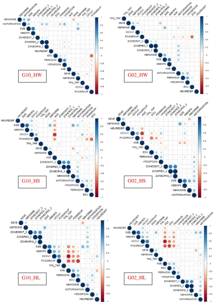
One of the common causes of the failure of regression model building is Multicollinearity between variables (see section 2.1.5). Determining and removing highly-correlated variables is a very important task to prepare proper data for model building. Below, the correlation matrices and variance inflation factors (VIFs and GVIF) are two common methods used to evaluate the independence between multiple variables for single-trip models. Values of GVIF exceeding 4 warrant further investigations, exceeding 10 are signs of serious multicollinearity while a value in correlation matrix (off-diagonal elements)) exceeding 0.9 is sometimes considered as a potential problem (Hair et al., 1998)

Table 16

Variance inflation factors of different motives in 2002 and 2010 (GVIF):

Variables/GVIF G10_HW G10_HS G10_HL G02_HW G02_HS G02_HL SEXE 1.407 1.335 1.271 1.426 1.371 1.319 AGE 1.210 2.766 3.714 1.163 2.378 3.280 PERMISOK 1.566 1.549 1.998 1.510 1.489 1.845 OCCU1 1.116 2.549 3.640 1.158 2.588 4.040 PCSGROUP 1.677 2.105 3.090 1.690 1.916 3.181 EDU 1.637 1.763 2.315 1.531 1.507 2.062 VPDISPOOK 1.760 1.587 1.537 1.482 1.549 1.558 SIZE 6.476 8.416 10.393 4.707 5.815 6.119 NBENF6 3.794 4.354 5.933 2.830 3.159 4.100 NBHOMME 2.568 3.012 3.269 2.099 2.238 1.938 NBFEMME 2.378 2.340 2.557 2.061 1.931 1.892 MOTORISATION 1.955 1.792 1.714 1.828 1.758 1.829 TPS_TRP 1.076 1.110 1.077 1.057 1.118 1.081 HEUREDEP 1.058 1.154 1.232 1.051 1.161 1.173

ZONERES_3 971.539 127.994 227.861 Infinite Infinite Infinite

Fig. 12: Correlation matrice for databases of different motives in 2002 and 2010

G10_HW G02_HW

G10_HS G02_HS

The correlation matrices and variance inflation factors (GVIF) show the high correlations between size and number of children above 6 years old, driving license and car availability, origin zone and residence zone, PCS group and education.

In studies about travel mode choice, a number of children above 6 years old, driving license, residence zone and PCS group appears to be less important than size, car availability, origin zone and education. So, we remove these variables from the database to avoid unwanted influence on our regression models.

Below is the table of final variable selection and variable definition of our research: Table 17

Name Symbol Unit Description Mode – single trips

MODE =1, if car =2, if public transport =0, others Mode – four-trip loops MODEB4 =1, if car =2, if public transport =3, if multimodal =0, others Gender SEXE =1, if female =0, otherwise Age AGE Years Age of individuals

Principal occupation OCCU1 =1, if full-time worker =2, if part-time worker =3, if pupil or student =0, otherwise Education level EDU

=1, if maternal or primary school =2, if secondary school =3, if high school =4, if university or higher =0, if not educated Car availability VPDISPOOK

=1, if own at least one car =0, otherwise

HH size SIZE Person Number of people a household has

Number of men NBHOMME Person Number of men a household has

Number of women NBFEMME Person Number of women a household has

Number of cars of HH MOTORISATION Car Number of cars a household owns

Travel time

TPS_TRP

Minute Duration of time which individuals spend during their trips

Departure time

HEUREDEP

Hour Hour of the time when individuals start their trips

Origin zone of trip

ZONEORIG_3

Zone where individuals leave from =1, city-center

=2, sub-urban =3, peri-urban