HAL Id: hal-00862442
https://hal.inria.fr/hal-00862442
Submitted on 16 Sep 2013
HAL is a multi-disciplinary open access
archive for the deposit and dissemination of
sci-entific research documents, whether they are
pub-lished or not. The documents may come from
teaching and research institutions in France or
abroad, or from public or private research centers.
L’archive ouverte pluridisciplinaire HAL, est
destinée au dépôt et à la diffusion de documents
scientifiques de niveau recherche, publiés ou non,
émanant des établissements d’enseignement et de
recherche français ou étrangers, des laboratoires
publics ou privés.
A Simple Broadcast Algorithm for Recurrent Dynamic
Systems
Michel Raynal, Julien Stainer, Jiannong Cao, Weigang Wu
To cite this version:
Michel Raynal, Julien Stainer, Jiannong Cao, Weigang Wu. A Simple Broadcast Algorithm for
Re-current Dynamic Systems. [Research Report] PI-2008, 2013. �hal-00862442�
Publications Internes de l’IRISA ISSN : 2102-6327
PI 2008 – September 2013
A Simple Broadcast Algorithm for Recurrent Dynamic Systems
Michel Raynal* Julien Stainer** Jiannong Cao*** Weigang Wu****
Abstract: This paper presents a simple broadcast algorithm suited to dynamic systems where links can repeatedly appear and disappear. The algorithm is proved correct and a simple improvement is introduced, that reduces the number and the size of control messages. As it extends in a simple way a classical network traversal algorithm (due to A. Segall, 1983) to the dynamic context, the proposed algorithm has also pedagogical flavor.
Key-words: Bounded delay, Broadcast, Distributed algorithm, Dynamic network, Mobile entity, Unbounded recur-rence, Recurrent link.
Un algorithme de diffusion pour les syst`emes dynamiques `a liens r´ecurrents
R´esum´e : Ce rapport pr´esente un algorithme de diffusion adapt´e pour les syst`emes dynamiques `a liens r´ecurrents, mais o `u la r´ecurrence n’est pas n´ecessairement born´ee.
Mots cl´es : Diffusion de messages, Lien r´ecurrent, Syst`eme dynamique.
*Institut Universitaire de France & IRISA (Rennes) (´equipe ASAP commune avec l’Universit´e de Rennes 1 et Inria) **IRISA (Rennes) (´equipe ASAP commune avec l’Universit´e de Rennes 1 et Inria)
***Department of Computing, Hong Kong Polytechnic University, Kowloon, Hong Kong
1
Introduction
Dynamic systems A fixed-process dynamic system is a system made up of a fixed number (n) of processes that communicate by sending and receiving messages through a point-to-point communication network whose structure varies with time. While the underlying communication network of a static system can be represented by a graph (each edge of which corresponding to a link), each link of a dynamic system can unceasingly appear and disappear. Moreover, the dynamic of the communication topology is not on the control of the system [15].
In an unreliable static system in which links can fail, the crash and the recovery of a link are considered as exceptional events, which must be appropriately processed (see, e.g., [1, 3, 18, 22]). Differently, as noticed in [10], in a dynamic system “the rate and the degree of the changes are generally too high to be reasonably modeled in terms of network failures: in these systems changes are not anomalies but rather integral part of the nature of the system”. As a simple example, one can consider the case of a mobile entity (process) whose moves disconnect it from some of its current neighbor entities and –at the same or a later time– reconnect it to other entities.
It is easy to see that, if changes occur permanently and too rapidly, nothing can be computed in a dynamic system (consider for example a 2-process system in which the link repeatedly appears and disappears without remaining up long enough to ensure message transmission). This means that, as soon as one wants to do non-trivial computations, dynamic system cannot be fully asynchronous. They must be constrained by synchrony/stability assumptions, whose power/strength may depend on the problem we are interested to solve. These assumptions capture synchrony/stability requirements which are sufficient to solve non-trivial problems. Examples of problems and assumptions which allow these problems to be solved despite the uncertainty created by dynamicity are consensus (e.g., [8, 11, 16]), leader election (e.g., [17]), and mutual exclusion [21]).
Broadcast in dynamic systems This paper focuses on the broadcast communication problem, namely, a process has to disseminate a data to the whole set of processes. This is a very basic problem whose solution allows the processes to compute any function F defined on their inputs. More precisely, each run has an input vector I[1..n] where I[i] represents the input value viof the process pi. Moreover, initially, I[i] = viis the only input value known by pi. The
broadcast abstraction allows each process to send its input value to all other processes, and then, each process can compute the function F(I) as soon as it has obtained the full input vector I.
A broadcast algorithm for dynamic networks is described in [14]. This algorithm assumes a synchronous dynamic system (processes execute collectively and synchronously a sequence of rounds) and, while the communication graph may change from round to round, the communication graph associated with each round must be connected. This algorithm is such that the processes can compute any computable function on their input vector in O(n2
) rounds and messages of size O(b + log n) where b is the number of bits needed to encode an input value.
Broadcast in dynamic networks is also addressed in [9] where different models of a dynamic system are considered. The main assumption of these models is that all the messages take exactly the same time to travel, hence transfer time is constant. Moreover this value is known by the processes. The presented models differ in the initial knowledge of the processes and the law governing the re-appearance of a link once it has disappeared (eventual, bounded, or periodic re-appearance).
Content of the paper This paper presents a simple broadcast algorithm suited to dynamic networks in which (a) message transfer delays are bounded by a constant δ (this bound δ can remain always unknown to the processes) and (b) when a link appears its lifetime is at least δ. Let us observe that an assumption on the minimal lifetime of links seems necessary (otherwise it is not possible to ensure that messages will ever be delivered). The algorithm shows that this assumption on link lifetime is sufficient.
In addition to the presentation of a broadcast algorithm suited to a dynamic distributed computation model, the paper has a pedagogical flavor in the sense that its construction is voluntarily “as close as possible” to the construction of a spanning tree –with a given root process– in a static system whose communication graph is connected [19]. Roadmap The paper is made up of 5 sections. Section 2 presents the dynamic distributed computing model. Sec-tion 3 defines the problems we are interested in (reliable broadcast and spanning tree construcSec-tion). SecSec-tion 4 presents
the algorithm, proves its correctness, and introduces improvements whose aim is to decrease the number and the size of control messages. Finally, Section 5 concludes the paper.
2
Dynamic System Model
In its most general sense, a dynamic distributed system is a system in which the number of processes can vary with time [2] and, in the case of message-passing systems, also the links (which allow processes to communicate) can vary with time [7]. We consider here the case of dynamic systems where the number of processes remains constant. Corresponding dynamic graphs have been introduced in [12]. Dynamic networks modeling these systems have been introduced in a lot of papers (under different names, e.g., evolving graphs [13], or time-varying graphs [6, 9], to cite a few). The readers will find nice introductory surveys related to dynamic systems in [10, 15]. These models of dynamic systems allow to take into account systems such as wireless networks, mobile networks, radio networks, etc.
Evolving graph [13] Let G(V, E) be a non-directed connected graph, SG = hG1, G2, . . . , GTi a sequence of its
subgraphs such that∪1≤i≤T = G , and ST = ht1, t2, . . . , tTi a sequence of time instants (whose length is the same
as SG). Let|V | = n (number of vertices and |E| = m (number of edges).
The tripleG = (G, SG, ST), where Giis the subgraph in place during the time period[ti−1, ti[ is called an evolving
graph.
The aim of an evolving graph is to model the behavior of a graph whose edges can repeatedly appear and disappear. The expressive power of time-varying graphs [10] is the same as the one of evolving graphs. (A time-varying graph associates with each edge of G a list of time intervals at which this edge exists.)
Process and communication model The system is made up of n processes, denoted p1, ... pn. The integer i, which
is called the index of pi, is used only for a notational purpose (a process pi does not know that its index is i). Each
process pihas an identity idi and knows only its identity and the fact that no two processes have the same identity.
The set of identities is not required to be structured by an order relation.
The processes communicate by sending and receiving messages through links. The set of current neighbors of a process piis defined by the graph Gxthat currently models the structure of the system.
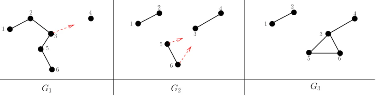
An example A simple example of an evolving graph that models the evolution of a set of six mobile processes (e.g., robots) is described in Figure 1. A process piis represented by its index i∈ {1, . . . , 6}. To simplify the presentation,
it is assumed that the process moves are instantaneously.
1 2 4 5 6 1 2 3 4 2 1 4 3 3 5 5 6 6 G1 G2 G3
Figure 1: Example of an evolving graph
The initial position is represented by the communication graph G1, in which p4is isolated. Then, p3moves (his is
represented by a small arrow attached to p3in G1), and becomes disconnected from p2and p5, and connected to p4.
The resulting communication graph is represented by G2. Then, both p5and p6move, and the communication graph
becomes G3, etc. It is important to see in this example that (a) none of G1, G2and G3is connected, (b) the graph
Permanent vs recurrent link A link that exists forever is a permanent link. A link that, after some finite time, exists forever, is an eventually permanent link. A link that appears and disappears infinitely often, is a recurrent link. It is assumed that the links which are not eventually permanent are recurrent, hence the term recurrent dynamic system. This assumption provides a “stability” property which allows algorithms to cope with the uncertainty created by the dynamicity of the system.
Let us remark that, due to the recurrence link assumption, the recurrent dynamic model is similar to the communi-cation model used in population protocols [4, 5].
Lower bound on link lifetime If, after a link has appeared, it can disappear at an arbitrary time, it is possible that no link remains present during a continuous long enough period and consequently all messages can be lost, from which follows that no non-trivial function can be computed. To prevent such a scenario from occurring, it is assumed that (a) there is an upper bound δ on message transfer delays, and (b) once a link appears, it remains present for at least δ time units. (A weaker assumption is presented in Section 4.2.)
It is assumed that a link incident to a process appears or disappears, this process is informed instantaneously. It follows that, if a process sends a message m on a link e when this link appears, this message is necessarily received by its destination process (and the sender knows this fact).
3
Reliable Broadcast and Construction of a Spanning Tree
Reliable broadcast Given a distinguished process pa, dynamically defined by the reception of an external message
denotedSTART(), the aim is to design an algorithm that allows pa to send a data to all the other processes of the
system.
Spanning tree construction In addition to the diffusion of an information, the algorithm has to build a spanning tree rooted at pa. Hence, at each process pi, the algorithm has to compute a pair of values denoted(parenti, childreni),
such that the set of pairs{(parenti, childreni)}1≤i≤ndefines a spanning tree of the system. Once computed, this
spanning tree can be used to broadcast values, elect a leader, etc.
4
A Simple Algorithm
4.1
The algorithm
Principle The algorithm consists in a straightforward extension (to the dynamic context previously described) of a basic broadcast and spanning tree construction, which is based on a simple flooding technique initially proposed in [20] in the context of static systems (see also Chapter 1 of [19] where are described several algorithms building a spanning tree in static systems).
The flooding technique is pretty simple. When it receives a data for the first time, a process forwards it to its current neighbors. But, as in a dynamic system, at any time, the set of current neighbors of a process pican be only a
subset of all its neighbors, pihas to additionally execute specific statements when a link (re-)appears, namely forwards
the data on this link if it is not sure that the destination process has a copy of this data.
As far as the construction of the spanning tree is concerned, a process defines its parent as the link on which it receives for the first time the data that has been broadcast. It computes its set of children when it receives messages from them, which inform it that they are its children.
Local variables The algorithm uses the following local variables at each process pi.
• As already indicated, at the end of the algorithm, parentiand childreniwill capture the position of pi in the
spanning tree. Initially, parenti= ⊥ (a default value), and childreni= ∅.
• current neighborsicontains the set of current neighbors of pi. It is assumed that when a link e incident to pi
appears or disappears, piis immediately informed of it.
Init:parenti← ⊥; childreni← ∅; notifyi ← ∅; visitedi← ∅;
current neighborsi ← set of edges connecting pito its current neighbors.
whenSTART(n) is received: % a single process receives this external message % (01) parenti← ⊤; nb proci← n; datai← data to be broadcast;
(02) for eache ∈ current neighborsido sendGO(datai) on e end for.
whenGO(d) is received on link e: (03) visitedi← visitedi∪ {e};
(04) if(parenti= ⊥) then
(05) parenti← e; datai← d;
(06) for eache′∈ (current neighborsi\ {e}) do sendGO(datai) on e′end for:
(07) notifyi ← {idi}; sendBACK(notifyi) on parenti
(08) end if.
whenBACK(nt) is received on link e:
(09) childreni← childreni∪ {e}; visitedi← visitedi∪ {e};
(10) notifyi← notifyi∪ nt;
(11) if(parenti= ⊤) % piis then the distinguished broadcasting process %
(12) then if(|notifyi| = nb proci− 1) then process piclaims termination end if
(13) else if(parenti∈ current neighborsi) then sendBACK(notifyi) on parentiend if
(14) end if.
each time the linke disappears:
(15) current neighborsi ← current neighborsi\ {e}.
each time the linke appears:
(16) current neighborsi ← current neighborsi∪ {e};
(17) if(parenti6= ⊥) then
(18) if(e /∈ visitedi) then sendGO(datai) on e; visitedi← visitedi∪ {e} end if;
(19) if(parenti= e) ∧ (notifyi6= ∅)
(20) then sendBACK(notifyi) on parenti;
(21) notifyi← ∅
(22) end if (23) end if.
Algorithm 1: A broadcast algorithm in a dynamic system with recurrent links
• visitediis a set (initially empty), which contains the links that connects pito neighbors that (to pi’s knowledge)
have received the broadcast value.
• dataiis used to save the value broadcast by the distinguished process pa.
• notifyi is a set (initially empty), which contains the identities of the descendants (in the spanning tree built so
far) of pi. This set is used to compute the value of childreni and allows the distinguished process pato learn
that the algorithm has terminated.
The algorithm Algorithm 1 implements a reliable broadcast and builds a spanning tree as follows. The algorithm starts when a (dynamically defined) process pareceives the external messageSTART(n). This process defines itself as
the root (this is encoded by parenti= ⊤), and sends to its current neighbors the messageGO(dataa) carrying the data
it wants to broadcast (lines 1-2). Let us remark that, thanks to the messageSTART(n), the distinguished process pa
learns n (the number of processes composing the system). This will allow it to detect the termination of the algorithm. Let us also remark that only paneeds to knows the value of n (line 12).
When a process pireceives a messageGO(d) on a link e, it first adds e to the set visitedi(line 3). If it is the first
time it receives this message, it defines e as its parent and forwards to its current neighbors the message it has just received (lines 4-6). Moreover, it also sends to its current parent, a notification messageBACK({idi}) to inform it that
it is one of its children. Let us observe that, according to appearance/disappearance of the link e, it is possible for the notification message to be lost.
A messageBACK(nt) carries a set of process identities, which are identities of descendents –with respect to the
spanning tree– of the receiving process pi. When it receives such a message, a process piadds first the corresponding
link e to its sets childreniand visitedi, and adds also the set nt it has received to its local set notifyi (lines 9-10).
Then if it is the distinguished process and it knows all its descendents in the spanning tree, pi claims termination
(lines 11-12). If it is not the root and it is currently connected to its parent (line 13), pisends its current information
on the tree (i.e., the set notifyi) to its parent. Let us observe that (as before) this notification message can be lost.
When a link e appears or disappears, piupdates accordingly the set current neighborsi(lines 15-16). When it is
a link appearance and pihas already received the broadcast data (hence, we have parenti 6= ⊥, line 17), it does the
following. If, from its point of view, the process to which it is connected by e has not received the broadcast data, pi
forwards it to it (line 18). Moreover, if the link e is the one connecting pito its parent in the spanning tree, pisends
the messageBACK(notifyi) to its parent to inform it of its descendent in the tree. This is to cope with the possible loss
of the previous messageBACK(notifyi) sent by piat line 7 or line 13. Let us notice that, due to the lower bound on
the lifetime on a link that appears, (if any) the messages sent at line 18 or line 20, cannot be lost. It follows that e can be safely added to visitediat line 18, and (because its content will be taken into account by its receiver) notifyi can
be reset to∅ (line 20).
4.2
A few remarks
Remark 1 let us notice that, while the distinguished root process eventually detects global termination (line 12), no other process can locally claim that its participation to the algorithm has terminated. This is due to the following reason. As link recurrence is not bounded, it is not possible for a process to know that it has communicated with all its neighbors in the graph G (union of the Gigraphs). This is a fundamental difference with corresponding algorithms
in static communication graphs. Adding an assumption such as an upper bound∆rec(known by each process) on the
appearance of each link would allow each process to know if it has locally terminated (this is because, after the first duration equal to∆rec, each process has been informed of all its neighbors in the graph G).
Remark 2 Assuming that the size of the data that is broadcast is bounded, all local variables and messages are bounded (their size depends only on the size of system). It is also important to notice that the bound δ (related to both the maximal transfer delay and the minimal continuous liftetime of a link) need not be known by the processes. It remains forever unknown to them.
Remark 3 It is easy to see that the algorithm can be modified so that it still works when only the links defining the final spanning tree are reliable (all the messages sent on the other links may be lost).
Remark 4 The assumption that, when it appears, a link exists during at least δ time units can be weakened as follows. When it appears, a recurrent link can now remain present for an arbitrary short period, but it is assumed that, infinitely often, it is present for more than2δ consecutive time units.
This weaker assumption is still valid, but requires additional statements. A message (GO() orBACK()) sent on a
link e has now to be acknowledged by its receiver. Moreover, each time the link e re-appears, the message sender must retransmit the message on this link, and this is repeated at each re-appearance of the link e until until the acknowledgment is received.
4.3
Proof of the algorithm
Let us remind that m is the number of edges of the communication graph.
Theorem 1. Algorithm 1 solves the broadcast problem and builds a spanning tree rooted at the broadcasting process, in the dynamic model with recurrent links. Moreover, the number of data messages (GO() messages) is upper bounded
by4m. The number of control messages (BACK() messages) is O(n2).
Proof The proof that every process receives a copy of the broadcast data follows from the following observation. If the link is alive at least δ time units after the data has been sent at line 2 or line 6, the messageGO(datai) is received by
its destination process. In the other cases (message loss due to link disappearance during the message transfer or link absent when line 2 or line 6 is executed), then it is re-sent at line 18 at the link re-appearance (which necessarily occurs due to link recurrence assumption). As the link is then alive for at least δ time units, the message is received. Let us finally observe that, as the communication network G is connected and the the messageGO(datai) are systematically
forwarded, every process eventually receives a messageGO(datai).
As far as the spanning tree is concerned we have the following. As each process receives at least one message
GO(datai) and defines its parent as the link on which it receives the first copy of this message, it follows that the sets
of variables{parenti}1≤i≤ndefines a tree rooted at the distinguished process. Moreover, as the messagesBACK(nt)
are sent only on the parent link, it follows that each set childreni contains only links from the children of pi. The
proof that at least one copy of each messageBACK(nt) sent at line 7, line 13, or line 20, is received is the same as for a
messageGO(datai). It follows that (a) the set of pairs {(parenti, childreni)}1≤i≤ndescribes a spanning tree of the
communication network G, and (b) the algorithm terminates (i.e., the root executes line 12).
Let us observe that a process sendsGO(datai) at most twice on a given link e (once at line 6 and once at line 18).
This is because we have parenti6= ⊥ after the first sending at line 6, which prevents another sending at the same line,
and the link is added to visitediafter the first sending at line 18. It follows thatGO(datai) is sent on a link at most
twice in each direction, from which we conclude that at most4m copies ofGO(datai) are sent.
Let us now look at the messagesBACK(nt). Each leaf pℓof the tree sends at most two messagesBACK(nt), with
idj∈ nt to its parent (one at line 7 and the other one at line 20). Such a message is then forwarded (line 13) up to the
root along the path from this leaf to the root of the tree. Moreover, for each non-leaf process pi, the same forwarding
may occur from pi to the root. It follows that the number of messagesBACK() depends both on the tree and on the
message exchange pattern. As, in the worst case, the tree is a line, it follows that the number of messagesBACK() is
upper bounded by O(n2
). ✷T heorem 1
4.4
Decreasing the number and the size of control messages
Useless messages According to the pattern of link appearances/disappearances, the previous algorithm does not prevent the same process identities from being sent several times from a process pi to its parent, while this is not
necessary. As an example, this occurs in the following scenario. Process pireceives a messageBACK(nt) and nt is
such that the set notifyi is not modified at line 10. Then, if pisendsBACK(notifyi) at line 13, not only the message
may be lost (due to the disappearance of link e), but its sending is actually useless.
Additional local variable To prevent useless messages BACK() from being sent, a new set is managed by each
process pi. The aim of this set, denoted already notifiedi and initialized to∅, is to contain pi’s descendents in the
spanning tree that are such that piknowsthat its parent has received their identities.
Improved algorithm Algorithm 2 is the corresponding improved version of Algorithm 1. The new lines are labeled **1 until **7, while all other lines are the same as in Algorithm 1.
The first (from an explanation point of view) added line is line **7. As (due to the lifetime of the link e, that just appeared) the messageBACK(notifiedi) sent at line 20 will be received by its destination process (the parent of pi),
piadds the set notifiedi to already notifiediso that the identities in notifiedi will not be sent again to the parent of
pi(line **7). This entails the addition (line **6) of the predicate¬(notifyi ⊆ already notifiedi) before the sending
issued at line 20.
The second improvement is the addition of the lines **2-**5, executed when a process pi receives a message
BACK(nt). The aim of these new lines is to prevent pi from executing the lines 11-14 (and consequently save the
Init:parenti← ⊥; childreni← ∅; notifyi ← ∅; visitedi← ∅;
current neighborsi← set of edges connecting pito its current neighbors;
(**1) already notifiedi ← ∅.
whenSTART(n) is received: % a single process receives this external message % (1) parenti← ⊤; nb proci← n; datai← data to be broadcast;
(2) for eache ∈ current neighborsido sendGO(datai) on e end for.
whenGO(d) is received on link e: (3) visitedi← visitedi∪ {e};
(4) if(parenti= ⊥) then
(5) parenti← e; datai← d;
(6) for eache′∈ (current neighborsi\ {e}) do sendGO(datai) on e′end for:
(7) notifyi← {idi}; sendBACK(notifyi) on parenti
(8) end if.
whenBACK(nt) is received on link e:
(9) childreni← childreni∪ {e}; visitedi← visitedi∪ {e};
(**2) previousi← notifyi;
(10) notifyi ← notifyi∪ nt;
(**3) notifyi ← notifyi\ already notifiedi;
(**4) if(previousi6= notifyi) then
(11) if(parenti= ⊤) % piis then the distinguished broadcasting process %
(12) then if(|notifyi| = nb proci− 1) then process piclaims termination end if
(13) else if(parenti∈ current neighborsi) then sendBACK(notifyi) on parentiend if
(14) end if (**5) end if.
each time the linke disappears:
(15) current neighborsi← current neighborsi\ {e}.
each time the linke appears:
(16) current neighborsi← current neighborsi∪ {e};
(17) if(parenti6= ⊥) then
(18) if(e /∈ visitedi) then sendGO(datai) on e; visitedi← visitedi∪ {e} end if;
(19) if(parenti= e)
(**6) ∧ ¬(notifyi ⊆ already notifiedi)
(20) then sendBACK(notifyi) on parenti;
(**7) already notifiedi ← already notifiedi∪ notifyi;
(21) notifyi ← ∅
(22) end if (23) end if.
Algorithm 2: Improved broadcast algorithm
5
Conclusion
The paper presented a simple broadcast algorithm suited to dynamic system with recurrent links. An improvement that reduces the size and the number of control messages has also been given.
This algorithm has been designed with a pedagogical flavor. It is a simple adaptation to a dynamic context restricted by synchrony assumptions of the classical algorithm proposed by A. Segall in the early eighties for static reliable asynchronous message-passing systems [20]. These additional synchrony assumptions concern the upper bound on message transfer delays, the link recurrence, and the minimal duration for the existence of each link each time it appears.
Acknowledgments
This work has been partially supported by the French ANR project DISPLEXITY devoted to computability and com-plexity in distributed computing. and the ANR France-Hong Kong project CO2DIM.
References
[1] Afek Y., Attiya H., Fekete A.D., Fischer M., Lynch N., Mansour Y., Wang D. and Zuck L., Reliable Communication over Unreliable Channels. Journal of the ACM, 41(6):1267-1297, 1994.
[2] Aguilera M.K., A Pleasant Stroll Through the Land of Infinitely Many Creatures. ACM SIGACT News, Distributed Computing Column, 35(2):36-59, 2004.
[3] Aguilera M.K., Chen W. and Toueg S., On quiescent reliable communication. SIAM Journal of Computing, 29(6):2040-2073, 2000.
[4] Angluin D., Aspnes J., Diamadi Z., Fischer M., and Peralta R., Computation in networks of passively mobile finite-state sensors. Distributed Computing, 18(4):235-253, 2006.
[5] Angluin D., Aspnes J., Eisenstat D., Ruppert E., The computational power of population protocols. Distributed Computing, 20(4): 279-304, 2007.
[6] Awerbuch B. and Even S., Efficient and reliable broadcast is achievable in an eventually connected network. Proc. 3rd ACM Symposium on Principles of Distributed Computing (PODC’84), ACM Press, pp. 278-281, 1984.
[7] Baldoni R., Bertier M., Raynal M., and Tucci Piergiovanni S., Looking for a definition of dynamic distributed systems. Proc. 9th Int’l Conference on Parallel Computing Technologies (PaCT’07), Springer LNCS 4671, pp. 1-14, 2007.
[8] Biely M., Robinson P., and Schmid U., Agreement in directed dynamic networks. Proc. 19th Int’l Colloqium on Structural Information and Communication Complexity (SIROCCO’12), Springer LNCS 7355, pp 73-84, 2012.
[9] Casteigts A., Flocchini P., Mans B., and Santoro N., Deterministic computations in time-varying graphs: Broadcasting un-der unstructured mobility. Proc. 5th IFIP Conference on Theoretical Computer Science (TCS), IFIP Advances in Inf. and Communication Technology Vol. 323 (Springer), pp. 111-124, 2010.
[10] Casteigts A., Flocchini P., Quattrociocchi W., and Santoro N., Time-varying graphs and dynamic networks. Int’l Journal of Parallel, Emergent and Distributed Systems, 27(5):387408, 2012.
[11] Coulouma E. and Godard E., A characterization of dynamic networks where consensus is solvable. Proc. 20th Int’l Col-loquium on Structural Information and Communication Complexity (SIROCCO’13), Springer LNCS aaaa, pp. aaaa-aaaa, 2013.
[12] Harary F. and Gupta G., Dynamic graph models. Mathematical Computer Modelling, 25(7):79-87, 1997. [13] Fereira A., Building a reference combinatorial model for MANETS. IEEE Network, 18(5):24-29, 2004.
[14] Kuhn F., Lynch N.A., and Oshman R., Distributed computation in dynamic networks. Proc. 42nd ACM Symposium on Theory of Computing (STOC’10), ACM press, pp. 513-522, 2010.
[15] Kuhn F. and Oshman R., Dynamic network: models and algorithms. ACM Sigact News, Distributed Computing Column, 42(1):82-96, 2011.
[16] Kuhn F., Moses Y., and Oshman R., Coordinated consensus in dynamic networks. Proc. 30th ACM symposium on Principles of Distributed Computing (PODC’11), ACM Press, pp. 1-10, 2011.
[17] Larrea M., Raynal M., Soraluze I., and Corti˜nas R., Specifying and implementing an eventual leader service for dynamic systems. Int’l Journal of Web and Grid Services, 8(3):204-224, 2012.
[18] Raynal M., Communication and agreement abstractions for fault-tolerant asynchronous distributed systems. Morgan & Clay-pool, 251 pages, 2010 (ISBN 978-1-60845-293-4).
[19] Raynal M., Distributed algorithms for message-passing systems. Springer, 500 pages, 2013 (ISBN 978-3-642-38122-5-2). [20] Segall A., Distributed network protocols. IEEE Transactions on Information Theory, 29(1):23–35, 1983.
[21] Walter J.E., Welch J.L., and Vaidya N.H., A mutual exclusion algorithm for ad hoc mobile networks. Wireless Networks, 7(6):585-600, 2001.
[22] Wang D.-W. and Zuck L.D., Tight Bounds for the Sequence Transmission Problem. Proc. 8th ACM Symposium on Principles of Distributed Computing (PODC’89), ACM Press, pp. 73-83, 1989.