HAL Id: hal-01653160
https://hal.archives-ouvertes.fr/hal-01653160
Submitted on 22 Apr 2020
HAL is a multi-disciplinary open access
archive for the deposit and dissemination of
sci-entific research documents, whether they are
pub-lished or not. The documents may come from
teaching and research institutions in France or
abroad, or from public or private research centers.
L’archive ouverte pluridisciplinaire HAL, est
destinée au dépôt et à la diffusion de documents
scientifiques de niveau recherche, publiés ou non,
émanant des établissements d’enseignement et de
recherche français ou étrangers, des laboratoires
publics ou privés.
numerical combustion
Cédric Mehl, Jérôme Idier, Benoit Fiorina
To cite this version:
Cédric Mehl, Jérôme Idier, Benoit Fiorina. Evaluation of deconvolution modelling applied to
nu-merical combustion. Combustion Theory and Modelling, Taylor & Francis, 2018, 22 (1), pp.38 - 70.
�10.1080/13647830.2017.1358405�. �hal-01653160�
Evaluation of deconvolution modelling applied to numerical
combustion
C´edric Mehl a∗, J´erˆome Idierband Benoˆıt Fiorinaa
aEM2C Laboratory, CNRS, CentraleSup´elec, Universit´e Paris-Saclay, Chˆatenay-Malabry, France; bLS2N, CNRS, Nantes, France
(Received 6 February 2017; accepted 8 July 2017)
A possible modelling approach in the large eddy simulation (LES) of reactive flows is to deconvolve resolved scalars. Indeed, by inverting the LES filter, scalars such as mass fractions are reconstructed. This information can be used to close budget terms of filtered species balance equations, such as the filtered reaction rate. Being ill-posed in the mathematical sense, the problem is very sensitive to any numerical perturbation. The objective of the present study is to assess the ability of this kind of methodology to capture the chemical structure of premixed flames. For that purpose, three deconvolution methods are tested on a one-dimensional filtered laminar premixed flame configuration: the approximate deconvolution method based on Van Cittert iterative deconvolution, a Taylor decomposition-based method, and the regularised deconvolution method based on the minimisation of a quadratic criterion. These methods are then extended to the reconstruction of subgrid scale profiles. Two methodologies are proposed: the first one relies on subgrid scale interpolation of deconvolved profiles and the second uses parametric functions to describe small scales. Conducted tests analyse the ability of the method to capture the chemical filtered flame structure and front propagation speed. Results show that the deconvolution model should include information about small scales in order to regularise the filter inversion. a priori and a posteriori tests showed that the filtered flame propagation speed and structure cannot be captured if the filter size is too large.
Keywords: deconvolution; large eddy simulation; laminar premixed flames; subgrid
scales; ill-posed problems
1. Introduction
As discussed in the review papers [1,2], the description of complex chemistry effects in Large Eddy Simulations (LESs) of reactive flows remains a key challenge for turbulent combustion modelling. A direct method is to use mechanisms where chemical reaction rates are modelled by Arrhenius-type laws. As this approach has been limited in the past to global step mechanisms, the prediction of pollutants formation as well as extinction or re-ignition phenomena was out of reach. However, thanks to tremendous progress in supercomputing, the LES of reactive flows in complex geometries and using analytical mechanisms is nowadays possible [3–5]. However, the LES filtered species balance equations exhibit unclosed terms that require accurate modelling, especially if the prediction of both flame dynamics and pollutant formation is desired.
∗Corresponding author. Email: [email protected]
C
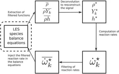
Figure 1. The concept of deconvolution modelling applied to LES.
As discussed in [6,7], Filtered Density Function (FDF) transport is a possible way to close filtered species balance equations whose chemical source terms are modelled by Arrhenius laws. The efficiency of these methods has been demonstrated on non-premixed jet flame configurations [8], but they are a priori not designed to capture the premixed or stratified flame dynamics encountered in many practical applications. Arrhenius-type laws can also be introduced in LES using the artificial thickened flame model [9,10], which ensures correct flame propagation in premixed regimes. However, flame thickening will bias the chemical flame structure, as discussed by Auzillon et al. [11].
Another possibility is to reconstruct reactive scalars from resolved filtered quantities.
Figure 1illustrates the application of this concept to filtered species reaction rates modelling. The variables ρ, Yk, and h are the filtered density, species mass fraction of the kth species,
and enthalpy transported by the LES flow solver, respectively. At each numerical iteration, unresolved variables ρ∗, Yk∗, and h∗ are reconstructed from filtered variables using a
deconvolution algorithm. Nonlinear functions, such as the chemical reaction rates ˙ωk, are
then computed using the deconvolved functions and explicitly filtered in order to estimate the filtered chemical reaction rate ˙ωkof the filtered species balance equations.
The critical step of the method is the deconvolution algorithm, which aims at recovering small-scale information. The application of deconvolution in LES has been pioneered by Stolz and Adams [12], who developed the Approximate Deconvolution Method (ADM). It was first applied to the modelling of subgrid-scale Reynolds stresses in non-reactive flows for different flow configurations [13,14]. A comprehensive review of deconvolution methods applied to non-reacting flow can be found in [15]. The first methods developed for reacting flows were derived from ADM. A coupling of ADM and a thickened flame has been done [16] and a modification of ADM based on scale similarity has led to a model for premixed flames [17]. A model based on the ADM formalism has also been derived for the specific case of non-premixed combustion [18,19]. More recently, two deconvolution algorithms have been proposed to tackle the closure of the equation regardless of the combustion regime. The first one consists in a Taylor expansion of the Gaussian filter [20] and the second one in the minimisation of a constrained quadratic function [21].
According to Mellado et al. [18], LES signals can be decomposed into three parts: (1) the resolved signal which corresponds to filtered quantities represented on the LES grid;
(2) the under-resolved scales for which frequency components are smaller than the cut-off frequency given by the LES filter size (approximately the grid size); and (3) the unresolved scales which correspond to scales smaller than the cut-off length scale, also called subgrid scales. The challenge of deconvolution in a practical LES grid is to recover the full signal composed of parts (1), (2), and (3) from the only data available at each LES iteration, i.e. the resolved signal (1). Deconvolution models recently introduced in the literature – ADM, Approximate Deconvolution and Explicit flame Filtering (ADEF) [20], and the Regularised Deconvolution Method (RDM) [21] – are designed to recover under-resolved scales (2) from resolved quantities (1). Additional effort is needed to include unresolved contributions (3).
Even though many studies of deconvolution applied to the LES of reactive flows have been carried out on three-dimensional configurations, the ability of this methodology to capture the laminar flame propagation speed and the chemical structure has never been investigated. Situations where the subgrid flame wrinkling is close to unity are common in practice and it is hence essential that a combustion model retrieves the correct flame dynamics in a laminar regime [2,22]. The suitability of existing methodologies will be challenged on the simple one-dimensional freely propagating flame configuration. The intent of this paper is not to provide the ultimate solution for applying deconvolution to combustion LES, but to analyse related issues. In particular, we aim to determine the importance of accounting for unresolved contribution (3) in the deconvolution process.
In the first part of the paper, the problem of deconvolution is presented and analysed. The chosen grid resolutions are representative of realistic LES meshes. The resolved (1), under-resolved (2), and ununder-resolved (3) contributions are illustrated through post-processing of a laminar flame. The second part is dedicated to deconvolution methods. Existing methods designed to recover under-resolved quantities (2) are first presented. Then, we propose two strategies to include unresolved contribution (3). The first one is simply based on linear interpolation whereas the second includes small scales with a parametric model.
All deconvolution methods are challenged on the one-dimensional freely propagating laminar premixed flame configuration in a priori and a posteriori analyses. An in-depth study of the laminar flame speed and its variation in time on a one-dimensional freely propagating CH4/air flame is finally done to highlight the importance of including small
scales in the modelling.
2. Deconvolution problem
2.1. The mono-dimensional filtered freely propagating flame configuration
The unstretched one-dimensional filtered laminar premixed flame configuration challenges the ability of the LES combustion model to capture the flame front propagation speed in situations where no wrinkling occurs at the subgrid scale. Under a unity Lewis number assumption and for isobaric conditions, the flame governing equations read
∂ρ ∂t + ∂ρu ∂x = 0 (1) ρ∂Yk ∂t + ρu ∂Yk ∂x = ∂ ∂x ! ρD∂Yk ∂x " + ˙ωk(Yk, T) (2) ρ∂h ∂t + ρu ∂h ∂x = ∂ ∂x ! ρD∂h ∂x " + ˙Q, (3)
where x is the direction normal to the flame front, ρ is the density, Ykis the species k mass
fraction, D the diffusivity coefficient, u the flow speed, T the temperature, and h the mixture enthalpy per unit mass. ˙Qis an energy heat loss term, neglected in the present work. These governing equations are filtered in an LES context, leading to
∂ρ ∂t + ∂ρ#u ∂x = 0 (4) ρ∂ #Yk ∂t + ρ#u ∂ #Yk ∂x = ∂ ∂x ! ρD∂Yk ∂x " + ˙ωk(Yk, T) + τk (5) ρ∂#h ∂t + ρ#u ∂#h ∂x = ∂ ∂x ! ρD∂h ∂x " + τh+ ˙Q. (6)
The overbar denotes the spatial filtering operation φ =$RG(x − u)φ(u) du, where φ is any thermo-chemical or flow quantity. G is called the filter kernel and is considered to be Gaussian throughout this article, so that G(x) =%6/π'2exp&−6x2/'2'. Details about
the implementation of the filter are given in AppendixA. The tilde operator denotes the density weighted filtering defined by ρ#φ= ρφ. Under the ideal gas assumption, the filtered density relates to the temperature T and the constant pressure p as follows: ρ = p/(rT, where r is the specific gas constant.
The unresolved convective terms of the species and energy balance equations, τkand
τh, read, respectively, τk = ∂ ∂x & ρ&#u#Yk− )uYk '' (7) τh= ∂ ∂x & ρ&#u#h− (uh''. (8) The diffusivity ρD = λ/Cp is modelled using a Sutherland type law: DT =
(µ0/Pr)(T/T0)α, where α = 0.682 , T0 = 300 K, µ0 = 1.8071 × 10⁻⁴ kg· s−1 · m−1,
and Pr = 0.68.
Chemical reaction rates are modelled by using the two-step methane mechanism de-scribed in [23]:
CH4+32O2−→ CO + 2H2O
CO +1
2O2←→ CO2.
(9) This 5-species/2-step mechanism is very simple but includes the main types of species encountered in most chemical mechanisms: reactants (CH4 and O2), products (H2O and
CO2) and CO, which is both an intermediate and a final product species. 2.2. Challenges of deconvolution for flames
2.2.1. Modelling and numerical issues
In a combustion LES context, the issues are to close Equations (4)–(6). The task is especially challenging for the filtered chemical reaction rates ˙ωk(Yk, T), as kinetic constants are
Figure 2. Comparison between the reference filtered reaction rate and the filtered reaction rate without a model for CH4and γ = 4. Solid lines: ˙ωCH4(Yk, T). Dashed lines: ˙ωCH4(#Yk, #T).
laminar problem, where the wrinkling of the flame by turbulence is not considered, the high nonlinearity of reaction rates induces critical issues.
This is illustrated inFigure 2, which shows the filtered chemical reaction rate of species CH4across a steady-state one-dimensional premixed laminar flame (the fresh gas velocity
exactly compensates the flame consumption speed in the reference frame of the flame). The dimensionless filter size is defined as γ = '/δr, where δr, the reactive flame thickness, is
defined as the Full Width at Half Maximum (FWHM) of the methane chemical reaction rate. The reference solutions (solid lines) are obtained by a priori filtering the chemical reaction rate extracted from the solution of the non-filtered flame equations Equations (1)–(3) for γ = 4. This solution is compared against a first-order approximation, where the chemical reaction rate is directly approximated from the resolved thermochemical quantities [24,25]: ˙ωCH4(Yk, T) ≈ ˙ωCH4(#Yk, #T) (the dashed lines in Figure 2). Important discrepancies are
observed between the reference and the first-order assumption, leading to a misprediction of the flame consumption speed of 46.7%.
When the LES grid is uniform with spacing 'x, the flame front resolution is defined as
n0 = δr/'x, where δris the filtered reactive flame thickness. As 'xis typically larger than
the flame thickness δr[26], deconvolved flame profiles are not sufficiently discretised on
the filtered simulation grid. Two methods are then possible: (i) use the same grid for LES and the deconvolution procedure [16,20,21,27], numerical diffusion will then compensate under-resolution of deconvolved profiles; or (ii) introduce a finer additional grid, dedicated only to the deconvolution procedure. This has been applied in the context of LES for non-reacting flows [28,29] but has never been investigated in a combustion context where the phenomena taking place at small scales are even more essential. This procedure will be investigated in the present work. The mesh is assumed uniform, with grid spacing '∗
x.
The deconvolved flame front resolution is then quantified by the parameter n∗
0, defined as
Figure 3. A priori computations of filtered flame propagation speed obtained from the integration of CH4filtered reaction rate ˙ωCH4profiles, as given by Equation (10). Each curve corresponds to a
given deconvolution profile resolution n∗
0. Results are plotted as a function of ϕ/δr, the dimensionless position of the flame relative to the grid cells.
The following analysis is conducted to highlight the impact of the deconvolved grid resolution on the flame structure: reference temperature and species mass fraction solutions, obtained by solving the system of Equations (1)–(3), are interpolated on grids with varying spacings '∗
x to mimic different deconvolved profile resolutions. The methane chemical
reaction rate is filtered and integrated across the spatial direction to estimate the filtered flame consumption speed:
S'c = 1 ρu(YCHb 4− YCHu 4)
* +∞
−∞
˙ωCH4(x) dx. (10)
In unsteady reactive computations, the flame position relative to the grid changes. Numerical resolution conditions may then evolve with time, especially when the reactive layer is under-resolved. To mimic a moving one-dimensional flame in the present a priori tests, the coarse mesh is shifted relative to the flame position by an offset distance ϕ. The filtered flame consumption speed is plotted inFigure 3as a function of ϕ/δrfor four different
grids. The flame speed varies periodically when n∗
0 is low, meaning that the deconvolved
profile resolution is not sufficient. Conversely, when n∗
0 grows the impact of the grid is
decreased. This highlights the importance of using a sufficient number of points for the deconvolved functions.
2.2.2. Filter and conditioning
The filtering operation is linear and is expressed as a matrix-vector multiplication ρYk=
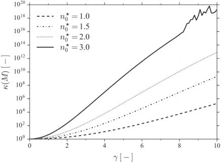
Figure 4. Computation of the condition number of M as a function of γ for different values of grid resolution n∗
0. A log scale is used for the condition number axis.
δ(ρYk)∗of the deconvolved function bounded by the following inequality:
)δ (ρYk)∗)
) (ρYk)∗) ≤ κ(M)
)δ(ρYk))
)ρYk)
, (11)
where the filter condition number κ(M) = )M))M−1) measures the sensitivity of the
deconvolution to a perturbation of the initial filtered function. If the condition number is close to one, the inversion of the filter is numerically stable. On the other hand, if it is larger than one, a perturbation of the initial filtered variable will cause a larger discrepancy on the deconvolved function.Figure 4 plots the condition number of M in terms of the dimensionless filter size γ for different grids resolutions n∗
0. The condition number grows
rapidly when the filter size increases, meaning that the problem is ill-conditioned. In addition, numerical stability issues are amplified when the resolution of the deconvolved profile increases.
2.2.3. Fourier analysis of the filtering operator
An analysis of LES filtering in terms of Discrete Fourier Transforms (DFTs) is proposed to understand modelling issues related to deconvolution methods. The analysis is done here using the CH4 mass fraction. The DFT vector for a given discretisation is given by the
points ! (ρYi)n= N+−1 m=0 (ρYi)mexp , −2πimnN -, (12)
Figure 5. Filtered and resolved CH4 mass fraction in Fourier space (γ = 5). Solid line: resolved
function | "ρYCH4|. Dashed line: filtered function | "ρYCH4|. Area with stripes: under-resolved part of
the signal. Area with points: unresolved part of the signal.
where N is the number of points in the spatial grid. A similar formula can be derived for filtered functions, hence enabling their frequency content to be compared. The filtering operator corresponds to a multiplication in Fourier space, therefore a transfer function is associated to each filter kernel. For a Gaussian filter, the DFT reads
.
ρYi(k) = e−'
2k2 .
ρYi(k), (13)
where k is the wavenumber.Figure 5plots the one-dimensional spectrum of both reference and filtered CH4mass fractions, extracted from a one-dimensional methane/air flame (with
φ= 0.8) in terms of the normalised wave number δrk. Low frequencies are almost unaffected
by the filtering operation whereas high frequencies are damped. The sub-filter contribution is shown by the area highlighted inFigure 5. As discussed in [18], two distinct contributions are identified: scales located to the left of the LES filter size wave number (the area with stripes) are damped by the filtering operation but are recoverable on the LES grid, whereas scales located to the right (the area with points) contain high-frequency components and are unrecoverable from the filtered LES signal.
2.3. Deconvolution methods
This section is dedicated to the presentation of deconvolution methods. Techniques designed to reconstruct the under-resolved part of the signal are described in Section 2.3.1 and methodologies to include unresolved contributions are discussed in Section2.3.2.
2.3.1. Deconvolution of under-resolved contributions
2.3.1.1 Approximate Deconvolution Method (ADM). One of the earliest attempts to use
deconvolution in LES is the ADM, originally proposed by Stolz and Adams [12]. It is based on Van Cittert’s algorithm and has been developed for non-reactive LES and focuses on the reconstruction of the recoverable part of the signal. This method, iterative and initialised using transported filtered quantities, reads
[ρYk]0= ρYk
[ρYk]n+1= [ρYk]n+ (ρYk− M [ρYk]n),
(14) where n refers to the iteration number. The deconvolved variables are approximated by
(ρYk)∗ = [ρYk]NADM, (15)
where NADMis the total number of iterations. In the variable density case treated here, the
filtered density ρ is deconvolved in a similar manner. As discussed in [12], NADM= 5 has
been retained in a good compromise between the computational cost and the accuracy of the model. ADM is a deconvolution method regularised by truncating the series. Indeed, low frequencies of the signal are recovered first and by stopping the series we avoid getting high frequencies, which are more sensitive to undesired perturbations.
2.3.1.2 Taylor decomposition of the filter. Domingo and Vervisch [20] proposed a
de-convolution method based on a Taylor-decomposition of the Gaussian filter. It aims at retrieving the recoverable part of scalars using the following deconvolution formulae:
(ρYk)∗= ρYk− '2 24 ∂2ρYk ∂x2 (16) (ρ)∗= ρ − '2 24 ∂2ρ ∂x2 (17)
Equation (17) is computed in practice by solving the anti-diffusion equation, explicitly or implicitly. The method, called Approximate Deconvolution and Explicit flame Filtering (ADEF), is a non-regularised method in the sense that no assumption is made about the deconvolved function.
2.3.1.3 The Regularised Deconvolution Method (RDM). Deconvolution can also be
per-formed by an optimisation process which aims at minimizing a quadratic criterion [21]: Yk∗ = min
s.t. Y− k≤Yk≤Yk+
)#Yk− #G∗Yk)2+ α)Yk− #Yk)2. (18)
The density is deconvolved by minimizing )ρ − G∗ρ)2. The deconvolution function
is constrained and a regularisation is performed via the addition of a penalisation term in the objective function. The approach is similar to a Tikhonov method [30,31]. The regularisation is based on the assumption that #Yk is an a priori assumed solution for the
deconvolved function Y∗
k. A similar approach has been used in a Conditional Source-term
Estimation (CSE) context [32]. Although this method was tested on the post-processing of a three-dimensional DNS, it will be challenged here on a coarse grid. The L-BFGS-B algorithm has been used to solve the optimisation problem (18) [33,34].
2.3.2. Extension to unresolved signal deconvolution
As discussed in Section2.2.1, the reconstruction of the unresolved part of a signal requires a reconstruction grid finer than the LES grid. Two alternatives are proposed to reconstruct this signal on the reconstruction grid: the first is a second-order interpolation, whereas the second extrapolates small-scale information by using a parametric model. The two strategies discussed in the following section are compatible with any of the deconvolution methods presented in the Section2.3.1.The methods described in Section 2.3.1 will also be referred to as explicit deconvolution methods in the next sections.
2.3.2.1 Second-order interpolation of the reconstructed signal. Second-order
interpo-lation inside each grid cell has been done in combination with the ADEF deconvolution method in the work of Domingo and Vervisch [20] and has also been studied in a TFLES context by Kuenne et al. [35]. A quadratic interpolation method will be used in the remainder of this paper.
2.3.2.2 Parametric reconstruction of subgrid scales. The quality of the second-order
interpolation can be improved by compensating for the remaining reconstruction error by a parametric model. The model relies on the self-similar properties of laminar flames, ob-served in multiple configurations, including premixed laminar [36] and premixed turbulent flames [37,38]. These self-similar properties suggest that subgrid-scale flame structures could be modelled by parametric analytical functions.
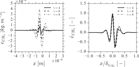
Density-weighted mass fractions obtained after explicit deconvolution and second-order interpolation are written (ρYk)∗, i. The method introduces an analytical function Mpk to model the remaining error ek = ρYk − (ρYk)∗, i. Similar patterns are observed when
computing ekfor different values of γ . This is illustrated inFigure 6, which shows on the
left the reconstruction error for ρYCH4obtained after application of the ADM deconvolution method. The normalised error ˆeCH4 = eCH4/max(eCH4) is plotted on the right inFigure 6as a function of a dimensionless spatial coordinate x/δeCH4. The curves superimpose, meaning
that a parametric model could be appropriate. The Gaussian modulated sine function is
Figure 6. Remaining error on CH4density-weighted mass fraction after application of the ADM
deconvolution method. On the left: absolute value. On the right: normalised value. Solid lines: γ = 4. Dashed lines: γ = 6. Dash–dotted lines: γ = 8.
employed to model Mpk:
Mpk(x) = Ae−b(x−x
0)2sin (2πf x + 2πϕ) , (19)
where x is the spatial direction; x0, A, b, f, and ϕ constitute a set of parameters that
charac-terise Mpk. These variables are identified during the deconvolution process by minimizing α, the difference between Mpk and the error ek:
α= min
pk )e
k− Mpk)
2. (20)
As ek is unknown, this optimisation process cannot be performed directly. However,
as the filtered variables are known, this optimisation step can be modified so that α is minimised:
α= min
pk )e
k− Mpk)
2, (21)
where ek= ρYk− (ρYk)∗,i. The final deconvolved function is then (ρYk)∗ = (ρYk)∗,i+
Mpk. This optimisation step is performed using a Newton-conjugate-gradient algorithm [39] on a fine grid of resolution n∗
0.
2.4. A priori analysis of deconvolution models
The deconvolution models are now challenged by post-processing the solutions of a filtered one-dimensional freely propagating laminar flame, discretised on a coarse grid in order to mimic realistic LES grid conditions.
The challenge of deconvolution is that the frequency range represented by the coarse grid is not large enough to capture the high frequencies contained in deconvolved functions. The a priori tests consist in post-processing a filtered laminar flame solution. In a first step, instantaneous solutions of the system of Equations (1)–(3) are selected as reference resolved data. In a second step, these solutions are filtered using the Gaussian filter operator. Finally, in a third step, the filtered data are deconvolved using one of the algorithms. Deconvolved data are then compared against the resolved reference solution. As a priori tests aim to evaluate the loss of information due to grid resolution and its impact on filtered reaction rates, it is especially important to use two different grids: a fine grid with spacing 'xfor
the variables used as the reference resolved solution and a coarse grid with spacing 'xfor
the filtered data. The coarse grid spacing 'x is defined such that 'x= δr/3, where δr is
the thickness of the filtered CH4reaction rate. This flame resolution is chosen to ensure a
proper prediction of the flame speed without introducing numerical artifacts. As the filtered flame thickness grows with the filter size, 'xincreases as well.
If the same grid were to be used, the inversion of perfectly filtered data using the same algorithm as the filter operator would lead to fake positive results. This numerical phenomenon, often referred in the literature as inverse crime, has to be considered when testing a deconvolution method [40]. A way of tackling the issue is to use additive noise [32]. In our case, as tests are done in realistic LES conditions (i.e. with a coarse grid for filtered variables), artificial noise is not needed.
The deconvolution models for under-resolved parts of signals are first tested and the impact of unresolved-scale modelling via interpolation and parametric functions is then studied.
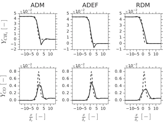
Figure 7. Deconvolved CH4and CO mass fractions for the three explicit deconvolution methods
(γ = 4). Solid lines: deconvolved term Y∗
k. Dashed lines: reference term Yk.
2.4.1. Deconvolution of under-resolved contributions
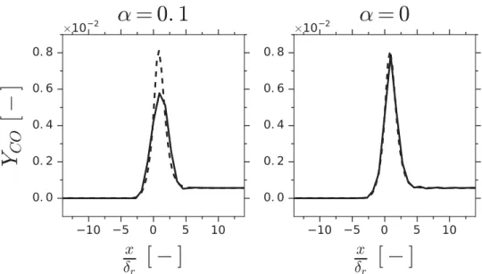
The dimensionless filter size is first set to γ = 4. Deconvolved mass fractions of methane and carbon monoxide are compared against resolved reference solutions inFigure 7. While the three deconvolution methods recover fairly well the reference solution for YCH4, only ADM and ADEF enable the CO peak to be correctly reproduced. The damping of the YCO
peak in the RDM solution may be due to the regularising term in Equation (18). This is demonstrated inFigure 8where the solution for α = 0.1 is compared to the solution with
α= 0 (no regularising term).
Further post-processing is performed to evaluate the ability of the methods to model the filtered chemical reaction rates, a key unclosed quantity. For that purpose, deconvolved reaction rates are first computed as ˙ω∗
k = ˙ωk(Yk∗, T∗) and filtered to obtain ˙ω ∗
k. This filtered
chemical reaction rate issued from the deconvolution procedure is compared to the reference one, obtained by filtering the reference resolved chemical reaction rate in Figure 9for both CH4 and CO. It shows that the three algorithms recover the correct shape of the
filtered methane reaction rate, though they slightly under-predict the peak. The task is more challenging for the CO chemical reaction rate, which exhibits both positive (production) and negative (consumption) contributions. ADM and ADEF do not even reproduce the shape of the profile. RDM succeeds in reproducing the shape, with however a misprediction of the negative peak.
Results are then shown for a higher filter size value, corresponding to γ = 8. The CH4and CO mass fractions are plotted inFigure 10, whereas the CH4 and CO chemical
Figure 8. Deconvolved CO mass fraction for the RDM deconvolution method with α = 0.1 (left) and α = 0 (right) for γ = 4. Solid lines: deconvolved term Y∗
k. Dashed lines: reference term Yk.
Figure 9. Modelled CH4and CO reaction rates for the three explicit deconvolution methods (γ =
Figure 10. Deconvolved CH4and CO mass fractions for the three explicit deconvolution methods
(γ = 8). Solid lines: deconvolved term Y∗
k. Dashed lines: reference term Yk.
Figure 11. Modelled CH4and CO reaction rates for the three explicit deconvolution methods (γ =
Figure 12. Error on laminar flame speed as a function of the filter size γ obtained after an
a priori analysis of explicit deconvolution methods. Triangles: approximate deconvolution method.
Circles: Taylor decomposition method. Crosses: regularised deconvolution method.
able to predict the CO peak. The CH4reaction rates are globally well captured, while big
discrepancies are exhibited for the CO reaction rates.
To quantify the impact of the deconvolution errors on flame front propagation, the deconvolved consumption speed is introduced:
S∗c = 1 ρu(YCHb 4− Y u CH4) * +∞ −∞ ˙ω∗ CH4(x) dx. (22)
The error (in %) on the laminar flame consumption speed is evaluated as .= 100 × | S ∗ c− S 0,ref l | Sl0,ref . (23)
The evolution of . with respect to the filter size γ is plotted inFigure 12. All methods behave correctly when γ is small. When γ increases, the flame speed is very sensitive to the loss of information due to filtering. For γ > 4, the evolution of the error is unstable. This is explained by the ill-conditioned nature of deconvolution: for different values of γ , different perturbations are seen by the algorithm and hence a high variability is observed in the results.
2.4.2. Deconvolution with unresolved-scale modelling
The same analysis is now carried out to study the effect of including information about fine scales using subgrid-scale interpolation and parametric functions. The small-scale ex-trapolation is done on a fine mesh of resolution n∗
Figure 13. Deconvolved CH4 and CO mass fractions for ADM (left), ADM with interpolation
(middle), and ADM with the parametric model (right) (γ = 4). Solid lines: deconvolved term Y∗ k.
Dashed lines: reference term Yk.
part, the methodology can be applied to any of the three explicit methods. Amongst the three methods presented previously, ADM is employed to retrieve under-resolved contributions.
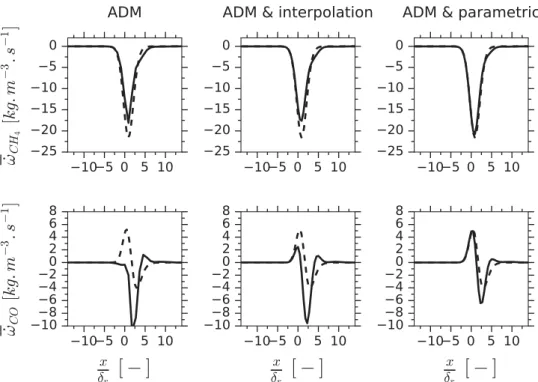
The impact of the parametric model is studied separately by first performing a de-convolution with subgrid-scale interpolation only and then a second dede-convolution with subgrid-scale interpolation and parametric modelling of reconstruction errors. Deconvolved CH4and CO mass fractions are shown inFigure 13for γ = 4, while the corresponding
reaction rates are plotted inFigure 14. Filtering is applied on the fine reconstruction grid. While the inclusion of the unresolved part of the signal with only second-order interpolation gives results similar to the method with no subgrid-scale modelling, the compensation of reconstruction error by a parametric model improves both the CH4reaction rate peak and
the CO reaction rate prediction.
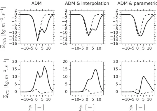
Similar conclusions are observed when considering a higher filter size (γ = 8), as shown inFigures 15and16. The CO mass fraction peak and the CH4 reaction rate are
better approximated by the inclusion of a parametric function. This is not the case for the CO reaction rate, for which even the unresolved-scale modelling via a parametric function cannot predict the correct shape. As γ increases, the conditioning of the deconvolution problem is affected and the unresolved part of the signal grows.
Finally, the impact of unresolved-scale modelling on the a priori laminar flame speed is illustrated: ., as defined in Equation (23), is plotted against γ inFigure 17. The addi-tion of an unresolved contribuaddi-tion to the reconstructed under-resolved signal with either
Figure 14. Modelled CH4and CO reaction rates for ADM (left), ADM with interpolation (middle),
and ADM with the parametric model (right) (γ = 4). Solid lines: modelled term ˙ω∗k. Dashed lines:
reference term ˙ωk.
Figure 15. Deconvolved CH4 and CO mass fractions for ADM (left), ADM with interpolation
(middle), and ADM with the parametric model (right) (γ = 8). Solid lines: deconvolved term Y∗ k.
Figure 16. Modelled CH4and CO reaction rates for ADM (left), ADM with interpolation (middle),
and ADM with the parametric model (right) (γ = 8). Solid lines: modelled term ˙ω∗k. Dashed lines:
reference term ˙ωk.
Figure 17. Error on laminar flame speed as a function of the filter size γ obtained after an a
priori analysis of deconvolution methods with unresolved-scale modelling. Triangles: approximate
deconvolution method. Circles: approximate deconvolution method with SGS interpolation. Crosses: approximate deconvolution method with SGS interpolation and the parametric model.
second-order interpolation or parametric modelling tends to improve the prediction of the flame consumption speed.
3. Filtered flame simulations using deconvolution algorithms
This section discusses the practical implementation of deconvolution algorithms to perform filtered flame simulations. The closure of the filtered reactive flow balance equations is given for one spatial dimension. Then simulation results of one-dimensional freely propagating filtered premixed laminar flames are shown and discussed.
3.1. Closing filtered species and energy balance equation using deconvolution
The RHS of the filtered species mass fractions balance equation (Equation5) is composed of three terms: the filtered chemical reaction rate, the unresolved convective fluxes and the filtered molecular diffusion. The RHS of the filtered energy equation (Equation 6), written under unity Lewis assumption, contains the filtered diffusion and the unresolved convective fluxes. To close species and energy balance equation budgets, filtered thermo-chemical variables ρYk, h, and ρ are first deconvolved to compute Y∗
k, ρ∗ and h∗ by
using one of the reconstruction algorithms described in Sec. 2.3. The deconvolved tem-perature T∗ is obtained from the deconvolved enthalpy h∗and the species mass fractions
Yk∗ by inverting the relationship h∗=/Nk=1h∗k(T∗)Yk∗ by using a Newton method. RHS terms are then closed by using the reconstructed thermo-chemical variables as discussed below.
Filtered chemical reaction rate ˙ωk
The species chemical reaction rate is first reconstructed at the subgrid scale by expressing chemical Arrhenius laws in terms of deconvolved variables:
˙ωk= ˙ωk(T∗, Yk∗) (24)
The filtered species chemical reaction rates of Equation (5) is then estimated by filtering explicitly the reconstructed chemical reaction rate:
˙ω(T , Yk) = ˙ω(T∗, Yk∗) (25)
Filtered laminar diffusive terms ∂ ∂x & ρD∂Yk ∂x ' and ∂ ∂x & ρD∂h∂x'
The diffusive terms of species Equation (5) and energy Equation (6) are estimated by the explicit filtering of the gradient of deconvolved variables Y∗
k, h∗, and D∗as follows: ∂ ∂x ! ρD∂Yk ∂x " = ∂ ∂x ! (ρD)∗ ∂Yk∗ ∂x " (26) ∂ ∂x ! ρD∂h ∂x " = ∂x∂ ! (ρD)∗ ∂h∗ ∂x " . (27)
The deconvolved molecular diffusivity is expressed as a function of the Prandtl number Pr and the flow viscosity µ: D = µ/Pr. By modelling the viscosity with the Sutherland law, we obtain (D)∗ =µ0 Pr ! T∗ T0 "α , (28)
where T0= 300 K is a reference temperature and α = 0.682.
Filtered laminar unresolved convective fluxes τk= ∂x∂ &ρ&#u #Yk− )uYk''and
τh= ∂x∂ &ρ&#u#h − (uh''
The relative local flame displacement speed Sd, defined as the difference between the
absolute flow speed u and the absolute flame front speed w, is introduced:
Sd = u − w. (29)
As the absolute flame front speed w remains constant across the flame brush, the filtered laminar species convective terms read
τk = ∂ ∂x & ρ&#SdY#k− )SdYk '' . (30)
By assuming that the steady-state regime is satisfied in the flame coordinate system, mass conservation implies the following relation between the laminar flame speed S0
l, the
fresh gas mixture density ρ0, and the local displacement speed:
ρSd = ρ0Sl0. (31)
This can be used to compute the terms in Equation (30): ρ#SdY#k = ρ0Sl0Y#k and ρ )SdYk=
ρSdYk= ρ0Sl0Yk. By introducing Yk∗, the filtered species unresolved laminar fluxes are
finally modelled as follows: τk= ∂ ∂x , ρuSl0 , # Yk− Yk∗ --. (32)
By analogy, the unresolved laminar fluxes of the energy balance equation read τh= ∂ ∂x & ρuSl0 &# h− h∗''. (33)
Summary of the model equations
The mass, species, and energy equations are finally modelled as ∂ρ
∂t + ∂ρ#u
ρ∂ #Yk ∂t + ρ#u ∂ #Yk ∂x = ∂ ∂x ! (ρD)∗ ∂Yk∗ ∂x " + ˙ωk(T∗, Yk∗) + ∂ ∂x , ρuSl0 , # Yk− Yk∗ --(35) ρ∂#h ∂t + ρ#u ∂#h ∂x = ∂ ∂x ! (ρD)∗ ∂h∗ ∂x " +∂x∂ &ρuSl0 &# h− h∗''. (36)
These equations are implemented into an in-house one-dimensional flame solver, which is 1st-order explicit in time and 2nd-order in space.
3.2. Results
Flame solutions obtained with methods for recovering the under-resolved part (2) of the signal are analysed first, while results which account for the unresolved part (3) of the signal are presented in a second part.
3.2.1. Deconvolution of under-resolved contributions
The fresh gas velocity is set to zero at the inlet of the domain. The grid is uniform with spacing 'x = δr/3. The system of filtered balance equations (34)–(36) is solved in time.
The computation is initialised with a filtered one-dimensional resolved flame. The analysis focuses on three quantities: the flame consumption speed S'
c, the filtered thermal thickness
#δth, and the maximal value of the CO mass fraction #YCOmax.
These three quantities are plotted as a function of the dimensionless time τ = δr/Sl0,ref
(where the reference flame velocity Sl0,ref is estimated from the laminar resolved flame solution) for γ = 1 and γ = 5 in Figures 18, 19 and20 for the three deconvolution methods recovering only under-resolved signals. At small filter size, the evolution of the three quantities in time is almost constant regardless of the deconvolution method used.
Figure 18. Flame consumption velocity as a function of time. Left: γ = 1. Right: γ = 5. Solid lines: parametric method. Dashed lines: ADEF. Dashed–dotted lines: ADM. Dotted lines: RDM.
Figure 19. Flame thermal thickness as a function of time. Left: γ = 1. Right: γ = 5. Solid lines: Parametric method. Dashed lines: ADEF. Dashed–dotted lines: ADM. Dotted lines: RDM.
Figure 20. Maximum of CO mass fraction as a function of time. Left: γ = 1. Right: γ = 5. Solid lines: Parametric method. Dashed lines: ADEF. Dashed–dotted lines: ADM. Dotted lines: RDM.
Only small variations are observed on the thermal thickness and the maximal CO mass fraction: relative variations of respectively 2.6 and 2.7% are for example observed for thermal thickness and maximal CO mass fraction when using the ADM method. The variations of the different quantities in time are significantly amplified when γ increases. The simulations exhibit spurious fluctuations up to 60% of the flame consumption speed. This is also the case for the CO mass fraction peak and the thermal thickness. These non-physical oscillations of flame speed, CO mass fraction peak, and thermal thickness when the filter size increases are due to the inability of ADM, RDM, and ADEF to reconstruct enough frequencies to define the deconvolved reaction rates accurately.
The performances of the deconvolution methods are then assessed for filter sizes in the range 1 < γ < 10. To simplify the analysis by still taking into account the unsteadiness of instantaneous quantities, a time-averaged flame consumption speed is hence defined:
< Sc'>= 1 T
* T 0
Figure 21. Error on flame consumption speed .'as a function of γ obtained by the simulation of
a one-dimensional laminar premixed flame. Triangles: approximate deconvolution method. Circles: Taylor decomposition method. Crosses: regularised deconvolution method.
where T is an integration time sufficiently large for < S'
c >to be statistically converged.
Note that time integration starts when the variation of flame consumption speed in time reaches a steady state. The error on the average flame consumption speed with respect to the reference speed is computed as follows:
.'= |< S ' c >−S 0,ref l | Sl,ref0 (38)
The relative peak-to-peak variation of consumption speed over time is also introduced:
δSc' =max 0
Sc'(t)1− min0Sc'(t)1
S0l,ref . (39)
As discussed in Section2.2.1, δS'
c is directly related to the flame resolution and is
expected to increase when the flame front resolution decreases. InFigures 21and22, .'and δS'
c, respectively, are plotted as functions of the
dimen-sionless flame filter size γ . When γ < 4, the methods lead to a good estimation of the mean flame speed < S0
l >, with an error below 5%. When γ > 4, the average consumption
speeds predicted by ADM, ADEF, and RDM deviate from the reference speed and the propagation is strongly affected by the modelling. When it comes to peak-to-peak flame speed fluctuations, the conclusions are similar. For γ < 3, δS'
c is lower than 8%, meaning
that it is acceptable to consider the laminar flame speed to be quasi-constant in time. It increases sharply for ADM, ADEF, and RDM when γ > 3. Regardless of the deconvolution method used, no satisfactory results are obtained for γ > 4.
Figure 22. Peak-to-peak variation of flame consumption speed δS'
c as a function of γ obtained by
the simulation of a one-dimensional laminar premixed flame. Triangles: approximate deconvolution method. Circles: Taylor decomposition method. Crosses: regularised deconvolution method.
A closer look at the performance of the different deconvolution methods reveals a similar behaviour between ADM and ADEF. This is explained by the fact that the grids used in the simulation are coarse and only permit the representation of low frequencies. The coarse grid regularises the deconvolution operation and the effect of the additional regularisation introduced by ADM is not significant. Only a slight advantage of ADEF over ADM is seen inFigure 22. The RDM method shows a better agreement with the average flame consumption speed but its evolution in time becomes very unstable as soon as γ > 6. A probable explanation lies in the ill-conditioning of the deconvolution, which makes the numerical optimisation of the regularised quadratic objective function (18) very difficult.
It should be noted that an important difference from the article of Wang and Ihme [21] and their implementation of the RDM methodology is the type of filter: a top-hat filter is used instead of a Gaussian filter. The condition number of a top-hat filter is very much lower than that of a Gaussian filter, and hence the numerical resolution is faster and more accurate. The drawback of the box filter is that it separates low and high frequencies less efficiently than a Gaussian filter, so that in realistic LES conditions many points are still required to correctly represent filtered functions.
3.2.2. Deconvolution with unresolved-scale modelling
3.2.2.1 Second-order interpolation of the reconstructed signal. Figures 23,24, and25
compare the evolution in time of S'
c, #δth, and #YCOmax, respectively, when using ADM and ADM with second-order interpolation at the subgrid scale. Results for γ = 1 are shown on the left of the figures while results for γ = 5 are on the right. The use of a fine reconstruction grid for representing small scales is important, as it limits the flame speed oscillations when the reactive layer crosses grid points. This corroborates the observations made onFigure 3.
Figure 23. Flame consumption velocity as a function of time. Left: γ = 1. Right: γ = 5. Dashed– dotted lines: ADM. Solid lines: ADM with SGS interpolation.
Figure 24. Flame thermal thickness as a function of time. Left: γ = 1. Right: γ = 5. Dashed–dotted lines: ADM. Solid lines: ADM with SGS interpolation.
Figure 25. Maximum of CO mass fraction as a function of time. Left: γ = 1. Right: γ = 5. Dashed–dotted lines: ADM. Solid lines: ADM with SGS interpolation.
Figure 26. Error on flame consumption speed .'as a function of γ obtained by the simulation of a
1-D laminar premixed flame. Triangles: Approximate Deconvolution Method.Circles: Approximate Deconvolution Method with SGS interpolation. Crosses: approximate deconvolution method with SGS interpolation and the parametric model.
Figure 27. Peak to peak variation of flame consumption speed δS'
c as a function of γ obtained by the
simulation of a 1-D laminar premixed flame. Triangles: Approximate Deconvolution Method. Circles: Approximate Deconvolution Method with SGS interpolation. Crosses: approximate deconvolution method with SGS interpolation and the parametric model.
Figure 28. Flame consumption velocity as a function of time. Left: γ = 1. Right: γ = 5. Dotted line: ADM with SGS interpolation only. Solid line: ADM with SGS interpolation and parametric modelling.
Figure 29. Flame thermal thickness as a function of time. Left: γ = 1. Right: γ = 5. Dotted line: ADM with SGS interpolation only. Solid line: ADM with SGS interpolation and parametric modelling.
Additionally, a stabilisation of the CO peak is also seen, although it is less pronounced for the flame thermal thickness.
The effect of SGS interpolation for different filter size values is analysed by studying the evolution of .'and δS'
c with γ inFigures 26and27. Deconvolution with unresolved-scale
modelling leads to a better prediction of the average flame speed, which remains almost constant as γ increases. Variations are also dramatically decreased; however, they become non-negligible when the filter size is large (δS'
c ≈ 20% for γ = 7). Indeed, when the filter
size grows, interpolation at the subgrid scale is not sufficient to represent the unresolved signal.
3.2.2.2 Parametric reconstruction of subgrid scales. The temporal variations of S'
c, #δth,
Figure 30. Maximum of CO mass fraction as a function of time. Left: γ = 1. Right: γ = 5. Dotted line: ADM with SGS interpolation only. Solid line: ADM with SGS interpolation and parametric modelling.
model are very close to the results with interpolation only, suggesting that the flame propagation improvement is due to the interpolation on the fine grid.
Errors on flame consumption speed and peak-to-peak fluctuations are added in
Figures 26 and 27, respectively. Improvements of the results by parametric modelling
observed in the a priori study are not significant. In practice, ill-conditioning of the decon-volution problem implies discontinuities in time of the reconstruction parameters.
Finally, the ability of deconvolution to capture the correct flame structure is studied. Steady-state solutions for the flame simulations with unresolved-scale modelling are shown onFigures 31,32, and33for γ = 2, 5, and 10, respectively. The classical ADEF, ADM, and
RDM deconvolution methods are very unsteady and are hence not considered here. Only the flames modelled with SGS modelling, which present low oscillations, are compared against the reference solutions. The simulations are analysed for a physical time t ≈ 10τ.
Figure 31. Comparison of filtered reference and deconvolved CH4 (left) and CO (right) mass
fractions for γ = 2 and t ≈ 10τ. Solid lines: ADM with parametric modelling. Dashed lines: ADM with SGS interpolation only. Dashed–dotted lines: filtered reference flame.
Figure 32. Comparison of the filtered reference and deconvolved CH4(left) and CO (right) mass
fractions for γ = 5 and t ≈ 10τ. Solid lines: ADM with parametric modelling. Dashed lines: ADM with SGS interpolation only. Dashed–dotted lines: filtered reference flame.
The comparison is made between the filtered flame computed with the deconvolution model and a filtered reference flame. All flames have been centred at x = 0.
For low filter sizes (case γ = 2), the flame structure is perfectly recovered. When the filter size has a medium value (γ = 5), the results are also good and both models are able to predict the correct flame. When the filter size becomes too high (γ = 10), there are strong discrepancies between the simulated and the filtered reference mass fractions. In particular, the CH4 mass fraction takes negative values (computation is made possible by clipping
these negative values) and is hence non-physical. This is the case for SGS interpolation alone and for the parametric model. In the case of parametric modelling, errors on CO are even more important, showing that, at these values of filter size, ill-conditioning of the optimisation problem leads to a deterioration of the results. Larger filter sizes lead to even lower negative values. This corroborates the observations made on Figure 27, where the difficulties encountered with deconvolution were revealed by the high value of δS'
c.
Figure 33. Comparison of the filtered reference and deconvolved CH4(left) and CO (right) mass
fractions for γ = 10 and t ≈ 10τ. Solid lines: ADM with parametric modelling. Dashed lines: ADM with SGS interpolation only. Dashed–dotted lines: filtered reference flame.
4. Conclusion
The objective of this article is to assess the ability of deconvolution to capture the flame propagation and chemical structure of laminar flames in an LES context. Approximations of non-filtered reactive scalars are found by applying a deconvolution algorithm to their transported (filtered) counterparts. The analysis focuses on the deconvolution algorithm, which is the critical modelling step in this new approach. It has been identified as a math-ematically ill-posed problem characterised by a high condition number. For that purpose, three reconstruction methods have been challenged. The first method proposed was de-signed for the modelling of the subgrid-scale Reynolds stresses in non-reactive LES and its extension to combustion has been tested here. Two other methods were specifically created for the closure of transport equations in a combustion context. The ADEF method uses the inversion of a Taylor decomposition of a Gaussian filter, whereas the RDM methodol-ogy solves a set of constrained and penalised quadratic functions at each iteration. These methods have been designed to retrieve the under-resolved part of a signal. New method-ologies including the influence of small scales are proposed. The main idea is to use a specific refined grid for representing deconvolved functions. A first methodology is based on the interpolation of deconvolved variables on the fine grid. An extension is then pro-posed, where a parametric model for small scales is added to compensate for the remaining errors.
A laminar one-dimensional premixed flame has been used to challenge the deconvolu-tion methods. This simple configuradeconvolu-tion enables us to study the nonlinearities due to the flame front independently from any turbulent effect. An a priori analysis was conducted first and showed a strong influence of the filter size on the results. When used on coarse LES grids with deconvolution methods intended to recover only the under-resolved sig-nals, the flame propagation speed and structure deviate from the reference value when the normalised filter size γ increases. Approximation of unresolved scales by interpolation improves the result even though it mostly fails at predicting the correct flame shapes. The parametric method shows a better agreement and is in particular able to get a better predic-tion of the CO peak and the species reacpredic-tion rates. A priori flame propagapredic-tion predicpredic-tions are however similar when using second-order interpolation or parametric modelling. A
posteriori analysis conducted on one-dimensional premixed flame simulations suggests the
same conclusions for the three methods that do not include small scales (RDM, ADEF, and ADM). They show large variation of flame consumption speed, CO peak, and thermal thickness over time. These variations increase with flame filter size. This is explained by the under-resolution of the LES grid and its inability to represent frequencies above its Nyquist frequency. Including unresolved information using second-order interpolation and a fine grid improves the stability of the flame front propagation, even though the method fails for large filter widths. Second-order interpolations are not significantly improved by the additional parametric compensation of the error.
The main conclusion of this study is that unresolved scales have to be accounted for in the deconvolution process in order to retrieve the laminar flame structure. As these small scales can only be represented on fine grids, the introduction of an intermediate refined grid for deconvolved variables is necessary. A CPU cost efficient extension of the present methods to multi-dimensional cases is a challenge for future work.
Disclosure statement
ORCID
C´edric Mehl http://orcid.org/0000-0003-2293-9281
References
[1] S.B. Pope, Small scales, many species and the manifold challenges of turbulent combustion, Proc. Combust. Inst. 34 (2013), pp. 1–31.
[2] B. Fiorina, D. Veynante, and S. Candel, Modeling combustion chemistry in large eddy
simulation of turbulent flames, Flow Turbul. Combust. 94 (2015), pp. 3–42. Available at
https://doi.org/10.1007/s10494-014-9579-8.
[3] T. Jaravel, E. Riber, B. Cuenot, and G. Bulat, Large eddy simulation of an industrial gas turbine
combustor using reduced chemistry with accurate pollutant prediction, Proc. Combust. Inst.
36 (2017), pp. 3817–3825. Available at https://doi.org/10.1016/j.proci.2016.07.027.
[4] B. Franzelli, E. Riber, and B. Cuenot, Impact of the chemical description on a large eddy
simulation of a lean partially premixed swirled flame, C. R. M´ecanique 341 (2013), pp. 247–
256.
[5] J. You, Y. Yang, and S.B. Pope, Effects of molecular transport in LES/PDF of piloted turbulent
dimethyl ether/air jet flames, Combust. Flame 176 (2017), pp. 451–461.
[6] D.C. Haworth, Progress in probability density function methods for turbulent reacting flows, 36 (2010), pp. 168–259. Available at https://doi.org/10.1016/j.pecs.2009.09.003.
[7] F. Gao and E. O’Brien, A large-eddy simulation scheme for turbulent reacting
flows, Phys. Fluids A: Fluid Dynamics 5 (1993), pp. 1282–1284. Available at
http://scitation.aip.org/content/aip/journal/pofa/5/6/10.1063/1.858617.
[8] Y. Yang, H. Wang, S.B. Pope, and J.H. Chen, Large-eddy simulation/probability density function
modeling of a non-premixed CO/H2 temporally evolving jet flame, Proc. Combust. Inst. 34 (2013), pp. 1241–1249.
[9] T.D. Butler and P.J. O’Rourke, A numerical method for two dimensional unsteady reacting
flows, Symp. (Int.) Combust. 16 (1977), pp. 1503–1515.
[10] P.J. O’Rourke and F.V. Bracco, Two scaling transformations for the numerical computation of
multidimensional unsteady laminar flames, J. Comput. Phys. 33 (1979), pp. 185–203.
[11] P. Auzillon, B. Fiorina, R. Vicquelin, N. Darabiha, O. Gicquel, and D. Veynante, Modeling
chemical flame structure and combustion dynamics in LES, Proc. Combust. Inst. 33 (2011),
pp. 1331–1338.
[12] S. Stolz and N.A. Adams, An approximate deconvolution procedure for large-eddy simulation, Phys. Fluids 11 (1999), pp. 1699–1701. Available at http://dx.doi.org/10.1063/1.869867. [13] S. Stolz, N.A. Adams, and L. Kleiser, The approximate deconvolution model for large-eddy
simulation of compressible flows and its application to shock–turbulent-boundary-layer inter-action, Phys. Fluids 13 (2001), pp. 2985–3001.
[14] S. Stolz, N.A. Adams, and L. Kleiser, An approximate deconvolution model for large-eddy
simulation with application to incompressible wall-bounded flows, Phys. Fluids 13 (2001),
pp. 997–1015.
[15] W. Layton and L.G. Rebholz, Approximate Deconvolution Models of Turbulence, Springer-Verlag, Berlin, 2012.
[16] J. Mathew, Large eddy simulation of a premixed flame with approximate deconvolution
mod-eling, Proc. Combust. Inst. 29 (2002), pp. 1995–2000.
[17] A.W. Vreman, R.J.M. Bastiaans, and B.J. Geurts, A similarity subgrid model for premixed
turbulent combustion, Flow Turbul. Combust. 82 (2009), pp. 233–248.
[18] J.P. Mellado, S. Sarkar, and C. Pantano, Reconstruction subgrid models for
nonpremixed combustion, Phys. Fluids 15 (2003), pp. 3280–3307. Available at
http://scitation.aip.org/content/aip/journal/pof2/15/11/10.1063/1.1608008.
[19] C. Pantano and S. Sarkar, A subgrid model for nonlinear functions of a scalar, Phys. Fluids 13 (2001), pp. 3803–3819.
[20] P. Domingo and L. Vervisch, Large eddy simulation of premixed turbulent combustion
us-ing approximate deconvolution and explicit flame filterus-ing, Proc. Combust. Inst. 35 (2015),
pp. 1349–1357. Available at https://doi.org/10.1016/j.proci.2014.05.146.
[21] Q. Wang and M. Ihme, Regularized deconvolution method for turbulent
com-bustion modeling, Combust. Flame 176 (2017), pp. 125–142. Available at https://doi.org/10.1016/j.combustflame.2016.09.023.
[22] B. Fiorina, R. Vicquelin, P. Auzillon, N. Darabiha, O. Gicquel, and D. Veynante, A filtered
tabulated chemistry model for LES of premixed combustion, Combust. Flame 157 (2010),
pp. 465–475.
[23] J. Bibrzycki and T. Poinsot, Reduced chemical kinetic mechanisms for methane combustion in
O2/N2and O2/CO2atmosphere, Working note ECCOMET WN/CFD/10/17, CERFACS (2010). [24] C. Duwig, K. Nogenmyr, C. Chan, and M.J. Dunn, Large eddy simulations of a piloted lean
premix jet flame using finite-rate chemistry, Combust. Theory Model. 15 (2011), pp. 537–568.
[25] C. Duwig and L. Fuchs, Lifted flame in a vitiated co-flow, Combust. Sci. Technol. 180 (2008), pp. 453–480.
[26] T. Poinsot and D. Veynante, Theoretical and Numerical Combustion, 2nd ed., R.T. Edwards, Philadelphia, PA, 2005.
[27] Q. Wang, H. Wu, and M. Ihme, Regularized deconvolution method for turbulent combustion
modeling, CTR Annual Research Briefs, Center for Turbulence Research, Stanford University,
California, 2015, pp. 65–75.
[28] J.A. Domaradzki and K.C. Loh, The subgrid-scale estimation model in the
phys-ical space representation, Phys. Fluids 11 (1999), pp. 2330–2342. Available at
http://link.aip.org/link/?PHFLE6/11/2330/1.
[29] J.A. Domaradzki, K.C. Loh, and P.P. Yee, Large eddy simulations using the subgrid-scale
estimation model and truncated Navier–Stokes dynamics, Theor. Comput. Fluid Dynam.
15 (2002), pp. 421–450.
[30] A.N. Tikhonov, Solution of incorrectly formulated problems and the regularization method, Soviet Math. Dokl. 4 (1963), pp. 1035–1038.
[31] A.N. Tikhonov and V.Y. Arsenin, Solutions of ill-posed problems, Math. Comput. 32 (1978), pp. 1320–1322.
[32] J.W. Labahn, C.B. Devaud, T.A. Sipkens, and K.J. Daun, Inverse anal-ysis and regularisation in conditional source-term estimation mod-elling, Combust. Theory Model. 18 (2014), pp. 474–499. Available at http://www.tandfonline.com/doi/abs/10.1080/13647830.2014.927076#.VYrEiPlVhBc. [33] R.H. Byrd, P. Lu, J. Nocedal, and C. Zhu, A limited memory algorithm for bound
con-strained optimization, SIAM J. Sci. Comput. 16 (1995), pp. 1190–1208. Available at
http://epubs.siam.org/doi/abs/10.1137/0916069.
[34] C. Zhu, R.H. Byrd, P. Lu, and J. Nocedal, Algorithm 778: L-BFGS-B: Fortran subroutines for
large-scale bound-constrained optimization, ACM Trans. Math. Softw. 23 (1997), pp. 550–560.
[35] G. Kuenne, A. Avdi´c, and J. Janicka, Assessment of subgrid interpolation for the source term
evaluation within premixed combustion simulations, Combust. Flame 178 (2017), pp. 225–256.
[36] G. Ribert, O. Gicquel, N. Darabiha, and D. Veynante, Tabulation of complex chemistry based on
self-similar behavior of laminar premixed flames, Combust. Flame 146 (2006), pp. 649–664.
[37] D. Veynante, B. Fiorina, P. Domingo, and L. Vervisch, Using self-similar
proper-ties of turbulent premixed flames to downsize chemical tables in high-performance nu-merical simulations, Combust. Theory Model. 12 (2008), pp. 1055–1088. Available at
http://www.tandfonline.com/doi/abs/10.1080/13647830802209710.
[38] B. Fiorina, O. Gicquel, and D. Veynante, Turbulent flame simulation taking advantage of
tabulated chemistry self-similar properties, Proc. Combust. Inst. 32 (2009), pp. 1687–1694.
Available at https://doi.org/10.1016/j.proci.2008.06.004.
[39] J. Nocedal and S.J. Wright, Numerical Optimization, Springer Series in Operations Research, Springer-Verlag, New York, 1999. Available at https://doi.org/10.1007/b98874.
[40] J. Kaipio and E. Somersalo, Statistical and Computational Inverse Problems, Springer-Verlag, New York, 2005.
Appendix A. Filter implementation
The work done in this paper only considered a Gaussian filter. It is widely used in reactive and non-reactive LES and is the only filter satisfying linearity, spacial invariance, isotropy, and scale invariance [15]. Several implementations of the Gaussian filter exist, and the most convenient way is probably to use Fourier transforms. This approach is however limited to uniform grids, and another method is used here. As an example, the filtering of ρ will be considered. We consider the following
diffusion equation for a function f:
∂f ∂t =
∂2f
∂x2. (A1)
If we take f(t = 0, x) = ρ(x), we have the following relationship: ρ(x) = f (t = '2/24, x). In
other words, Gaussian filtering is equivalent to diffusing the function. The time integration of (A1) is done using an Euler implicit scheme with Nite= 20 iterations.