HAL Id: hal-02268377
https://hal.archives-ouvertes.fr/hal-02268377
Submitted on 20 Aug 2019
HAL is a multi-disciplinary open access
archive for the deposit and dissemination of
sci-entific research documents, whether they are
pub-lished or not. The documents may come from
teaching and research institutions in France or
abroad, or from public or private research centers.
L’archive ouverte pluridisciplinaire HAL, est
destinée au dépôt et à la diffusion de documents
scientifiques de niveau recherche, publiés ou non,
émanant des établissements d’enseignement et de
recherche français ou étrangers, des laboratoires
publics ou privés.
Debris-flow release processes investigated through the
analysis of multi-temporal LiDAR datasets in
north-western Iceland
Costanza Morino, Susan Conway, Matthew Balme, John Hillier, Colm Jordan,
Þorsteinn Sæmundsson, Tom Argles
To cite this version:
Costanza Morino, Susan Conway, Matthew Balme, John Hillier, Colm Jordan, et al.. Debris-flow
release processes investigated through the analysis of multi-temporal LiDAR datasets in north-western
Iceland. Earth Surface Processes and Landforms, Wiley, 2019, 44 (1), pp.144-159. �10.1002/esp.4488�.
�hal-02268377�
Debris-flow release processes investigated through
the analysis of multi-temporal LiDAR datasets in
north-western Iceland
Costanza Morino,1* Susan J. Conway,2 Matthew R. Balme,3 John Hillier,4 Colm Jordan,5 Þorsteinn Sæmundsson6and Tom Argles1
1School of Environment, Earth and Ecosystem Sciences, The Open University, Walton Hall, Milton Keynes MK7 6AA, UK 2CNRS UMR 6112 Laboratoire de Planétologie et Géodynamique de Nantes, Université de Nantes, 2 rue de la Houssinière, 44322
Nantes, France
3School of Physical Science, The Open University, Walton Hall, Milton Keynes MK7 6AA, UK 4Department of Geography, Loughborough University, Loughborough LE11 3TU, UK
5British Geological Survey, Environmental Science Centre, Keyworth, Nottingham NG12 5GG, UK
6Department of Geography and Tourism, University of Iceland, Askja, Sturlugata 7, IS-101 Reykjavík, Iceland
Received 12 July 2017; Revised 25 July 2018; Accepted 12 August 2018
*Correspondence to: Costanza Morino, School of Environment, Earth and Ecosystem Sciences, The Open University, Walton Hall, Milton Keynes, MK7 6AA, UK. E-mail: costanza.morino@open.ac.uk
This is an open access article under the terms of the Creative Commons Attribution License, which permits use, distribution and reproduction in any medium, provided the original work is properly cited.
ABSTRACT: Debris flows are fast-moving gravity flows of poorly sorted rock and soil, mixed and saturated with water. Debris-flow initiation has been studied using empirical and experimental modelling, but the geomorphic changes, indicative of different trigger-ing processes, are difficult to constrain with field observations only. We identify signatures to disttrigger-inguish two different debris-flow release styles by integrating high-resolution multi-temporal remote sensing datasets and morphometric analysis. We analyse debris flows sourced above the town of Ísafjörður (Iceland). Two debris-flow triggering processes were previously hypothesised for this site: (i) slope failure, characterised by landslides evolving into debris flows; and (ii) the fire-hose effect, in which debris accumulated in pre-existing, steep-sided bedrock passages is transported by a surge of water. It is unknown which process dominates and determines the local risk. To investigate this question, we compare airborne LiDAR elevation models and aerial photographs collected in 2007 with similar data from 2013. We find that two new debris-flow tracks were created by slope failures. These are characterised by steep sliding surfaces and lateral leveed channels. Slope failure also occurred in two large, recently active tracks, creating the preparatory conditions for the fire-hose effect to mobilise existing debris. These tracks show alternating zones of fill and scour along their length, and debris stored below the source-area at rest angles>35°. Our approach allows us to identify and quantify the morphological changes produced by slope failure release process, which generated the preparatory conditions for the fire-hose effect. As debris flows are rarely observed in action and morphological changes induced by them are difficult to detect and monitor, the same approach could be applied to other landscapes to understand debris-flow initiation in the absence of other monitoring information, and can improve the identification of zones at risk in inhabited areas near hillslopes with potential for debris flows. © 2018 The Authors. Earth Surface Processes and Landforms published by John Wiley & Sons Ltd.
KEYWORDS: debris flow; release styles; LiDAR; multi-temporal analysis; NW Iceland
Introduction
Debris flows are rapid (e.g. 0.8–28 m s-1; Rickenmann, 1999) and potentially destructive mass movements composed of a co-hesionless mixture of water and poorly sorted sediments (Iverson, 1997). To initiate, debris flows require the availability of unconsolidated material, excess moisture to saturate and mobilise this material, and slopes greater than 15°–20° (Costa, 1984; Terzaghi et al., 1996; Rickenmann, 1999; Imaizumi et al., 2006). Hundreds of thousands of cubic metres of sedi-ment can be transported for distances of over tens of
kilometres, even on moderate (~5–10%) gradients (Iverson, 1997; Rickenmann and Koschni, 2010). They are distinct from other forms of landsliding due to their periodic occurrence on established paths, usually in gullies or first- order drainage channels (Hungr et al., 2014).
Debris flows can initiate in several ways, e.g. by shallow translational or rotational sliding (Innes, 1983; Costa, 1984), by the erosion and mobilisation of accumulated material on hillslopes or in pre-existing depressions (Davies, 1986; Cannon et al., 2001), or by sediment entrainment in channels (Hungr et al., 2005). Different styles of triggering and propagation
Earth Surf. Process. Landforms44, 144–159 (2019)
© 2018 The Authors. Earth Surface Processes and Landforms published by John Wiley & Sons Ltd. Published online 20 September 2018 in Wiley Online Library
processes of debris flows have inherently different precondi-tioning factors. It is important to understand which triggering processes (or combination of processes) are active during the formation and evolution of debris flows to anticipate their be-haviour in zones exposed to their hazard, and hence to design mitigation and prevention measures.
Direct observation of the initiation processes of debris flows is the best way to identify them, but is seldom possible. In re-cent years, the development of high-resolution topographic data from laser scanning (or “LiDAR”, Light Detection And Ranging) and photogrammetric datasets has facilitated the study of debris flows. Monitoring of debris flows through multi-temporal LiDAR data is becoming more and more com-mon, particularly for sediment budget analysis and for study-ing debris-flow initiation (Scheidl et al., 2008; Bull et al., 2010; Blasone et al., 2014; Bossi et al., 2015; Cavalli et al., 2017). Bremer and Sass (2012) used a combination of terres-trial laser scanning (TLS) and airborne laser scanning (ALS) to quantify and map the sediment volume transported by a single debris-flow event in the Austrian Alps. Erosion and deposition generated by channel-bed entrainment of sediments by debris flows in the Swiss Alps have been calculated by differencing two ALS digital elevation models (DEMs) (Frank et al., 2015). Loye et al. (2016) used time series TLS data to quantify the sediment budgets of two debris-flow events in the Manival catchment (France). They were able to distinguish between the seasonal debris recharge produced by rockfall in winter, and the debris produced by hillslope sediment reworking in spring and autumn. In the same area, Theule et al. (2015) used TLS to quantify erosion and deposition caused by debris flows, and ALS to detect unstable sediment deposits that could be a source for new events. In all these studies, the number of the debris-flow events was known and the debris-flow catchments were monitored by other means. However, when catchment changes are not easily identifiable– in the absence of moni-toring systems or witnesses– knowing how and when individ-ual or multiple debris-flow events occur is challenging. A possibility that has not been fully explored in literature is the identification and quantification of different debris-flow re-lease processes from multi-temporal laser altimetry datasets, in which the conditions for their development are poorly monitored.
Here, we investigate how two debris-flow initiation pro-cesses (slope failure and fire-hose effect, which have been pre-viously proposed for our study area in the Westfjords of Iceland; Decaulne et al., 2005; Conway et al., 2010) manifest them-selves in terms of geometric properties and geomorphological features recognisable and measurable in remote sensing data. Specifically, we quantify the geomorphic effects of debris flows on the slope above the town of Ísafjörður through the comparison of two repeat aerial photograph and airborne laser altimetry datasets from 2007 and 2013. In particular, we use the airborne LiDAR data to calculate the volumes eroded and deposited along debris-flow tracks by potential multiple debris-flow events, and we couple these volume quantifica-tions with the analysis of changes in slope and geomorphic observations and interpretations from the aerial photographs. This allows us to assess and distinguish the role of two release mechanisms in debris-flow generation: slope failure and fire-hose effect.
Identifying and characterising different debris-flow processes is useful for understanding both sediment cascades and the im-plications of the potential hazard posed by debris flows where they occur near inhabited areas. This can be achieved by LiDAR differencing, which in our case has permitted the detec-tion and quantificadetec-tion of debris accumulated at high gradients without the assistance of any other monitoring system or
information on the evolution of the hillslope. From remote sensing interpretation alone, we do not know if one or several debris-flow events have mobilised the material between 2007 and 2013 in the tracks that we analyse, but this debris could be the source-material for potentially larger debris flows in the future. This kind of study, implemented with in situ channel survey and monitoring, can improve both our understanding of how debris flows develop and mitigate the risks associated with them.
Debris-flow activity in the study area
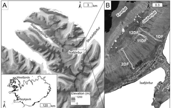
Slopes in the north-western region of Iceland, the Westfjords (Figure 1(A)), are prone to debris flows (Decaulne, 2005). Ísafjörður is the largest town of the peninsula, with a population of approximately 2600 inhabitants over an area of 4.2 km2in 2016. It has more than 150 buildings (including a hospital, two schools, two elderly residences, and three kindergartens) less than 50–300 m from recently emplaced debris-flow runout deposits. Although in this century debris flows have not caused major loss of life in the Westfjords, they do pose a serious haz-ard to local infrastructure and population (Decaulne, 2004). In mid-June 1999, six debris flows occurred after a sudden and in-tensive snowmelt period on the slope overlooking the town of Ísafjörður, damaging houses and infrastructure (Decaulne et al., 2005). Moreover, at least 24 debris-flow events occurred on this slope between 1900 and 1999, giving a return period for debris flows of 4–5 years (Decaulne et al., 2005).
Our study site is located above the town of Ísafjörður in the Gleiðarhjalli area, situated on the western side of the Skutulsfjörður fjord (Figure 1(A)). The fjord was shaped by Pleistocene-age glaciers and is carved into the Tertiary Basalt Formation, comprised of 2 to 30 m thick jointed basaltic lava flows separated by lithified sedimentary horizons (from a few centimetres up to tens of metres thick; Thordarson and Hoskuldsson, 2002), which are gently dipping towards the south-east (Kristjánsson et al., 1975; Sæmundsson, 1980).
The Gleiðarhjalli bench, which is located on the south-eastern side of Eyrarfjall Mountain at a height of 470 m above sea level (a.s.l.) on average, is 1500 m long and 450 m wide at maximum (Figure 1(B)). Deposits of poorly sorted glacial till 20–35 m thick (surveyed and measured by visual inspection in the field) are perched on this bench (Figure 2(A)), at whose margin they are unstable. The till deposits are composed of subangular to subrounded clasts varying in size from pebbles to metre-scale boulders and lying in a matrix of clay, silt and sand. The deposits are covered by centimetre to metre-sized angular clasts from talus deposits, which are either lying scattered on the bench or leaning against the rockwall (Figure 2(B)). Chutes (i.e. steep-sided passages scoured in bedrock along which the debris flows can move) are incised into the exposed rockwall at the edge of the bench (Figure 2(B)), forming areas through which most of the transfer of sediment to the lower parts of the slopes takes place.
The SE-facing hillsides above Ísafjörður have steep slopes in the range 25° to 35°, and slightly concave profiles. Below the exposed rockwall, the slope is covered by talus material and relict debris-flow deposits (Figure 2). Grass, moss and patches of dwarf birches and bilberries (30–40 cm high) cover the slope of Ísafjörður on its lower part. Trees are absent, apart from two small artificially forested areas at the foot of the slope (covering ~43 000 m2 and 6800 m2, respectively), planted with spruce (3–4 m high on average) as wind-breaks and for aesthetic rea-sons. The lack of substantial vegetation in the upper part of the slope favours erosional processes (Elwell and Stocking, 1976; Wells, 1981, 1987).
In Ísafjörður, heavy and prolonged rainfall and rapid snow-melt have been recognised as the main factors that promote rapid mass wasting phenomena, which are also favoured by
the steepness of the slope (Decaulne and Sæmundsson, 2003, 2007; Sæmundsson et al., 2003). However, the exact physical mechanisms by which debris flows are initiated have been
Figure 1. (A) The study area in the Icelandic Westfjords. Elevation data are from the Digital Elevation Model over Europe (EU-DEM) from the Global Monitoring for Environment and Security service for geospatial reference data access project (GMES RDA). (B) Aerial photograph shows the town of Ísafjörður, with debris flows analysed in this study marked with white outlines. [Colour figure can be viewed at wileyonlinelibrary.com]
Figure 2. South-east flank of the Eyrarfjall mountain above the town of Ísafjörður showing the four debris-flow tracks analysed for this study (debris flow 2DF in (A), debris flows 1DF, 11DF and 12DF in (B)). Above the rock cliff it is possible to observe talus fans and perched deposits on the Gleiðarhjalli bench; chutes are scoured in the bedrock below the bench ridge and the debris flows’ channels incise the deposits from talus material and relict debris flow deposits. Arrows and dashed lines indicate the migration of the channels of 1DF and 2DF in the terminal parts, leaving fan-shape debris accumulation. Some of the runout depositional lobes reach the inhabited areas. The white dotted line marks an example of chute area, the white indented line an example of crown overlying the main failure scarp. Photograph taken on July 26, 2013. [Colour figure can be viewed at wileyonlinelibrary.com]
hypothesised but not studied in too much detail. This is par-tially due to the difficulties in accessing and observing the phe-nomena directly, which is only rarely possible in Ísafjörður (Decaulne et al., 2005), and other mountain environments (Berti et al., 1999; McArdell et al., 2007; Coe et al., 2008).
Among the many possibilities, two processes are most com-monly considered responsible for triggering debris flow here: slope failure and the fire-hose effect (Decaulne et al., 2005; Conway et al., 2010). Initiation by slope failure is characterised by one or more discrete slope failures, instigated by changes in pore water pressure due to gradual in situ infiltration of rain or snowmelt (Hungr et al., 2001). As failure proceeds, contraction of debris causes an excess in pore water pressure, weakening the debris mass and resulting in the transformation from local-ised failure into a debris flow (Iverson, 1997). It is believed that this initiation style is experienced in the Gleiðarhjalli area; Decaulne et al. (2005) observed that intense precipitation and snowmelt caused saturation of the debris mantle covering the bench. Decaulne et al. (2005) further observed that the debris flows begin with rockfalls originating from the edge of the bench. This implies a subsequent loss of support, leading to the perched deposits sliding and then forming channelised de-bris flows. The authors report that, between the rock-fall phase and the debris-flow phase, the uppermost part of the tracks were temporarily blocked by the collapsed material from up-slope, being prone to be re-mobilised by further events.
Initiation by the fire-hose effect (Johnson and Rodine, 1984) is characterised by a concentrated flow of water that entrains loose deposits, which are generally located in a steep bedrock channel, torrent or chute (Godt and Coe, 2007). An increase in pore-water pressure results in their conversion into a debris flow (Johnson and Rodine, 1984; Coe et al., 1997; Griffiths and Webb, 2004). The recurrence interval of such flows is con-trolled by the debris accumulation rate in the source area and the timing of triggering precipitation. The fire-hose effect has been inferred to have been active in the Westfjords based on field inspections (Decaulne and Sæmundsson, 2006; Conway et al., 2010), but has never been fully characterised and quantified.
Methods
Dataset-processing and Digital Elevation Model
generation and interpolation
In 2007 and 2013, the UK Natural Environment Research Council’s Airborne Research Facility Data Analysis Node (NERC-ARF-DAN) collected aerial photography and LiDAR data for Súgandafjörður and Skutulsfjörður areas in Iceland. De-tails of both aerial surveys are reported in Table I. As the methods of remote sensing data collection differed between the two years, including the location/type of the reference GPS base stations on the ground, the two LiDAR datasets needed further processing to attain a satisfactory comparison. Alignment and filtering are required when comparing different types of datasets, in order to achieve sufficient accuracy for
producing volumetric differencing (Bremer and Sass, 2012; Roberti et al., 2017). Furthermore, co-registration error between flightlines needs to be corrected. Approaches such as morpho-metric parameter distributions (Sofia et al., 2013) or spatially variable error models (Schaffrath et al., 2015) have been devel-oped to correct these errors. Fuzzy inference system (Fis) has also been used to estimate the spatial variability of elevation uncertainty in individual DEMs, in order to propagate the un-certainties into the so-called DEM of Differences (DoD) map (Moss, 2000; Scheidl et al., 2008; Theule et al., 2012; Blasone et al., 2014; Bossi et al., 2015), and then assess the significance of the propagated uncertainty (Wheaton et al., 2010; Bangen et al., 2016; Cavalli et al., 2017). The iterative closest point (ICP) algorithm has successfully been used to improve co-registration errors where data from individual flightlines can be used (Besl and McKay, 1992; Chen and Medioni, 1992; Zhang, 1994). The correction is based on a least squares adjust-ment (similar to that of Akca, 2007), which matches the surface shape between each track to individually align the tracks rela-tive to a reference point cloud (Brasington et al., 2000; Lane et al., 2003; Milan et al., 2007). The ICP procedure allows the alignment between two point clouds to be as close as possible (James and Robson, 2014; Micheletti et al., 2015). Since we have reliable LiDAR data collected in 2013, and we could use this as the reference elevation dataset for aligning the 2007 LiDAR flightline (s), we chose to apply ICP procedure. In order to assess the DEM accuracy, we assumed the propa-gated DEM uncertainty in the DoD as uniform, and determined a minimum level of detection, above which changes were con-sidered to be real (Brasington et al., 2000, 2003; Fuller et al., 2003). This approach has been successfully used in recent an-alogue case studies (Bossi et al., 2015; Cavalli et al., 2017).
The 2007 LiDAR point data have horizontal and vertical shifts of up to 2 m between flightlines caused by a lack of between-track corrections in the initial processing (such errors are particularly problematic in steep terrain, see Favalli et al. (2009) for a full analysis). The 2013 data by comparison have averagely 6 cm vertical and horizontal differences between overlapping flightlines. We used only one flightline from the 2007 LiDAR data and cropped out the area of interest in order to reduce the errors from the LiDAR data processing. Cropping the dataset into a relatively short along-track segment (1.5 km) reduces the errors introduced by poorly integrated flight navi-gation and positional information. We then corrected the mis-alignment between the 2013 and 2007 datasets by means of the open source CloudCompare software, using an implemen-tation of the ICP algorithm. We used the point cloud from the 2013 LiDAR data as the reference data for the 2007 data, as the 2007 cloud had more severe co-registration issues. Once corrected, the mean value of the normal distances of the 2007 point cloud from the 2013 reference is 0.49 m (standard deviation 0.28 m); from the value of 0.49 m we defined our minimum level of detection as ±0.5 m.
After the co-registration, we imported the point clouds into ArcGIS and gridded the LiDAR data at 1 m/pixel, using the re-turn time of the last peak of light to reach the receiver from the LiDAR laser shot, which is generally assumed to be the ground return. To do so, we used the LAStools extension for
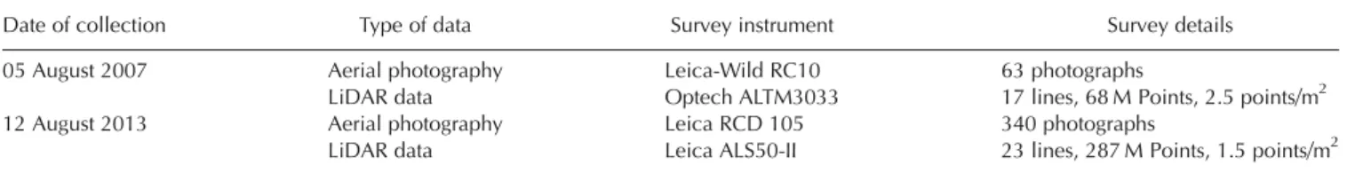
Table I. Details of airborne survey of Súgandafjörður and Skutulsfjörður fjords for year 2007 and year 2013
Date of collection Type of data Survey instrument Survey details 05 August 2007 Aerial photography Leica-Wild RC10 63 photographs
LiDAR data Optech ALTM3033 17 lines, 68 M Points, 2.5 points/m2 12 August 2013 Aerial photography Leica RCD 105 340 photographs
ArcGIS, which temporarily triangulates the LiDAR points into a Triangulated Irregular Network (TIN), and then rasterises the TIN into a Digital Elevation Model. The rasters were con-structed so as to be orthogonal, i.e. so that the pixel-size and pixel-centres were the same. Finally, using ArcGIS, we calcu-lated elevation changes and volumes by subtracting the 2007 gridded data from the 2013 data, producing the DoD.
DEM of difference error propagation
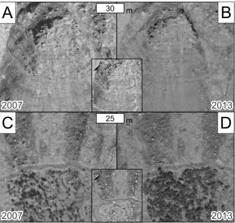
Any individual errors in the DEMs derived from the LiDAR, generated during surveying and post-processing, are propa-gated into the DoD (Goulden and Hopkinson, 2010). The DoD error varies spatially and arises from factors such as steep-ness of the terrain (causing data-gaps), the growth/change of dense vegetation, the varying density of the point clouds (data-gaps or false-smoothing) or misalignment between datasets (which causes an increase in error with the measure-ments between different datasets; Reuter et al., 2009). On the majority of the hillslope of Ísafjörður, between 2007 and 2013 there are few changes in elevation above the minimum level of detection (less than 0.5 m vertical change for 89% of the area analysed), and those that do occur are usually caused by noise or artefacts in the data (Figure 3(A)–(D)). Figures 3(A) and (B) show areas with no observable differences in the aerial photo-graphs between 2007 (Figure 3(A)) and 2013 (Figure 3(B)), yet detectable differences in the DoD. Apparent elevation changes of up to ±5 m in the DoD are caused by the steepness of the bedrock cliff– where different (sub-pixel) horizontal positions of the laser spots between years result in large differences in the height values. Artefacts with a magnitude of ±2.5 m can be caused by growth and/or changes in vegetation, but such example can be easily identified by comparison with the aerial photographs (Figure 3(C)–(D)).The deposited and eroded
volumes along and within the debris-flow tracks are key met-rics in this study, so we explicitly derived the effects of errors on our volume calculations, using the DoD to determine the relative absolute and percentage errors in the estimates (Table II). First, we manually selected areas lacking visible change from aerial photographs (‘stable areas’) and with similar setting (i.e. slope angles and vegetation/materials) to the analysed debris flows, and we calculated their volume changes. We then divided the volumes of the sampled debris flows obtained from the DoD by the area of the selected zones that showed no changes in the aerial images, and multiplying the results by the area of the sampled debris flows. The volume error calculated with this approach depends on the scale of the process (when the uncertainty on the measurements have min-imum values, errors are not proportional to the measurement), so errors are low for medium-scale flows (volumes between 1000 and 100 000 m3; Innes, 1983), ranging between ±3% and ±5% for deposited volumes and ±4% for eroded volumes. Small-scale flows (volumes of 1–1000 m3; Innes, 1983) often have higher relative error because they cover smaller areas and mobilise less material, giving calculated errors of ±9– 11% for deposited volumes and ±5–7% for eroded volumes. Particularly high values of error occur where small volume flows cover large spatial areas. Furthermore, some of the error values for volumes are relatively large (see Table II), because we have used a fixed vertical uncertainty, so zones whose vol-ume values are dominated by vertical changes with magnitudes close to that of the minimum level of detection (±0.5 m) have large percentage errors.
Track selection, naming and segmentation
We studied four debris-flow tracks on the slope above Ísafjörður (Figure 1(B)). We adopted and extended the naming protocol
Figure 3. Aerial photographs from 2007 (left side) and 2013 (right side) of a portion of the steep cliff above Ísafjörður (A, B) and of the forest on ESE side of the town (C, D) showing different sources of noise in the map of difference in elevation (in the centre, see Figure 5 for legend). Noise has been cleaned by checking for changes in the aerial photographs and distinguishing the signal. [Colour figure can be viewed at wileyonlinelibrary.com]
for debris-flow tracks used in Conway et al. (2010), who stud-ied debris flows in the same area. They named 10 debris-flow tracks using numbers from 1 to 10 followed by the acronym ‘DF’. As two of the debris-flow tracks coincide with two tracks analysed in this study, namely debris flows 1DF and 2DF, we used those names. We continued the same numbering system for two newly developed debris flows: debris flows 11DF and 12DF (Figure 1(B)).
We selected these four tracks because they show substantial (>±0.5 m) geomorphic changes between 2007 and 2013 in the differenced LiDAR datasets. These include morphological changes in the chutes at the front edge of the Gleiðarhjalli bench and in the upper part of the channels. We focused our analysis at these locations, being the zones of the debris flows where the majority of the changes occurred. Two of the four tracks, 11DF and 12DF (Figure 2(B)), did not exist in the 2007 data. The other two, 1DF and 2DF tracks (Figure 2(A)–(B)) were already present in 2007, but they had changed their form by 2013. Because 1DF and 2DF are different from 11DF and 12DF in their size, mor-phology and the processes that controlled their formation (as discussed below), we treat the two pairs of debris flows sepa-rately in the‘Results’ and ‘Discussion’ sections.
Having differenced the LiDAR datasets, we observed that, within the four debris-flow tracks, elevation changes occur in clearly defined, down-flow spatial domains. Since the debris-flow tracks present an atypical distribution of volumes, we seg-mented them and outlined different subareas according to the predominance of negative or positive elevation change from vi-sual inspection; for example, negative elevation change was predominant in the upper part of 2DF track, so we split it from the strongly contrasting area below, characterised by a positive change in elevation (see Figure 5(A) in‘Results’ section). This in turn allowed us to calculate the eroded and deposited volumes for these subareas and for the debris-flow tracks as a whole (see Table II in‘Results’ section).
2007
–2013 comparison
To analyse the changes occurring along each debris-flow track, we adopted the following approaches:
(i) to evaluate the deposited and eroded volumes within each debris-flow track, we derived the volumetric changes in these zones (i.e. debris-flow tracks and debris-flow subareas);
(ii) we visually identified geomorphological changes that oc-curred along the tracks in aerial photographs. Additionally,
we performed repeated field observations (summer 2012, 2013, 2016) in order to check what we observed and mapped from remote sensing;
(iii) we created a slope map at 1 m/pixel using the standard tools provided in Spatial Analyst of ArcGIS; the slope angle was derived using the steepest downhill slope as calculated by fitting a plane through the eight nearest neighbours (neighbourhood slope algorithm, also known as the average maximum technique; Burrough et al., 2015). Slope was evaluated for each subareas of the four debris flows: we took topographic profiles along the line of steepest descent, then extracted both the elevation values and the slope values for both the 2007 and 2013 DEMs along those lines.
Results
Morphology and morphometry of debris-flow tracks
1DF and 2DF
1DF and 2DF are the largest debris-flow tracks analysed in this study, having mobilised volumes up to 14 times larger over areas up to 8 times wider than 11DF and 12DF (see dimen-sional details in Table II). They are deeply incised and have chutes carved in bedrock in their upper part, with channels cut-ting slope deposits (Figure 2). In their terminal parts it is possi-ble to observe fan-shaped debris accumulations (Figure 2). Over the whole debris-flow tracks, total erosion volumes are larger than their total deposition volumes. 1DF has an erosion volume more than twice the depositional volume, while 2DF has 25% less deposition than erosion over the whole volume mobilised (see Table II). The net sediment budget should be near zero, but the deposits of the terminal lobes that reached the defensive protections were removed by the local authorities.
1DFa and 2DFa: most of the erosion in 1DF and 2DF occurs in their upper subareas (designated as ‘a’), namely in the perched material at the edge of the bench and in the apical chutes carved into the bedrock. Erosion occurs in subareas 1DFa and 2DFa, amounting respectively to 5622 ± 132 m3 and 3601 ± 28 m3(Figures 4(B) for 1DF, 5(B) for 2DF, Table II),
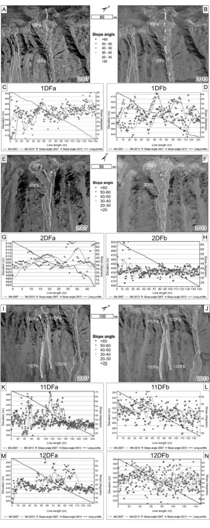
over a great range of slope (Figure 6). For both the debris-flow tracks in the time span between 2007 and 2013, the slope angle below the scarps and in the apical chutes remains on average above 35° (Figure 6(A)–(H), Table III). Erosion is also ev-ident from the morphology of the upper subareas 1DFa and
Table II. Results of the measured eroded and deposited volumes and other parameters of debris flows Debris flow ID Erosion
(m3) Error (m3) Error (%) Deposition (m3) Error (m3) Error (%) Area (m2) Maximum lenght (m) Chute width (m) Elevation drop (m) Debris flow 1DF 8552 ± 322 ± 4 4079 ± 223 ± 5 23952 803 125 406 Subareas ID 1DFa 5622 ± 132 ± 2 629 ± 91 ± 15 9845 168 - -1DFb 256 ± 31 ± 12 2234 ± 21 ± 1 2300 129 - -1DFc 2674 ± 159 ± 6 1216 ± 110 ± 9 11807 506 - -Debris flow 2DF 5001 ± 183 ± 4 3760 ± 127 ± 3 13596 727 74 411 Subareas ID 2DFa 3601 ± 28 ± 1 63 ± 19 ± 31 2077 51 - -2DFb 201 ± 43 ± 22 3058 ± 30 ± 1 3225 156 - -2DFc 1198 ± 111 ± 9 639 ± 77 ± 12 8294 520 - -Debris flow 11DF 862 ± 46 ± 5 339 ± 32 ± 9 3394 325 29 235 Subareas ID 11DFa 832 ± 31 ± 4 70 ± 21 ± 30 2303 187 - -11DFb 30 ± 15 ± 49 269 ± 10 ± 4 1091 138 - -Debris flow12DF 628 ± 42 ± 7 271 ± 29 ± 11 3131 286 32 207 Subareas ID 12DFa 549 ± 24 ± 4 82 ± 16 ± 20 1777 137 - -12DFb 78 ± 18 ± 23 188 ± 13 ± 7 1354 149 -
-Figure 4. (A) Elevation-difference map of debris-flow track 1DF obtained calculating the difference in elevation that occurred between 2007 and 2013, overlying the hillshade model derived from 2013 LiDAR. (B) Maps of the erosion and deposition distribution of debris-flow track 1DF derived by differencing the LiDAR generated topography from 2007 and 2013. The debris flow was segmented in subareas of prevailing erosion and depo-sition along its length. Distal lobes extensively modified during protection works (Figure 10) are omitted to avoid confusion. (C-F) Aerial photographs of the upper zones of debris flows 1DF, 11DF and 12DF from 2007 (C) and 2013 (D) compared, with simplified sketches of the main observable fea-tures (E and F, where the hillshade models derived from 2007 and 2013 LiDAR data, respectively, are overlain by aerial photographs in transparency). [Colour figure can be viewed at wileyonlinelibrary.com]
Figure 5. (A) Elevation-difference map of debris-flow track 2DF obtained calculating the difference in elevation that occurred between 2007 and 2013, overlying the hillshade model derived from 2013 LiDAR. (B) Maps of the erosion and deposition distribution of debris flow track 2DF derived by differencing the LiDAR generated topography from 2007 and 2013. The debris flow was segmented in subareas of prevailing erosion and depo-sition along its length. Distal lobes extensively modified during protection works (Figure 10) are omitted to avoid confusion. (C-F) Aerial photographs of the upper zones of debris flow 2DF from 2007 (C) and 2013 (D) compared, with simplified sketches of the main observable features (E and F, where the hillshade models derived from 2007 and 2013 LiDAR data, respectively, are overlain by aerial photographs in transparency). [Colour figure can be viewed at wileyonlinelibrary.com]
Figure 6. Aerial photographs of the upper zones of debris flows from 2007 (A, E, I) and 2013 (B, F, J) showing the steepest slope lines with colour indicating the slope values. Below, plots of the slope angles from 2007 (in red) and 2013 (in blue) against the long profile representing the terrain el-evation in 2013 (black continuous line) for subareas‘a’ (C, J, K, M) and ‘b’ (D, H, L, N). Red and blue continuous lines indicate the moving average (MA, interval 1°) for year 2007 and 2013 respectively. [Colour figure can be viewed at wileyonlinelibrary.com]
2DFa. In 1DFa in 2007, tension cracks, associated with areas of erosion located directly below them, cut the bench above the crown (Figure 4(C), (E)), with three more appearing in 2013, concomitant with enlarged erosion areas (Figure 4(D), (F)). In 2DFa, the main failure scarp in 2013 originated from two al-ready well defined release scarps that since 2007 regressively eroded 22 m (Figures 5(E), (F); note the paler material marking the main scarp below the crown in Figure 5(D)). Tension cracks that are present above the crown in 2DFa in 2007 had been partially erased by regressive erosion by 2013. Springs rise at the contact between the deposits perched on the bench and the underlying bedrock (Figure 5(D), (F)).
1DFb and 2DFb: immediately below 1DFa and 2DFa, posi-tive elevation change of up to ~5 m occurs in the chutes and in the upper channels (Figure 4(A) for 1DF, 5(A) for 2DF). The majority of the accumulated deposits of 1DF and 2DF, 2234 ± 21 m3and 3058 ± 30 m3respectively (Table II), lie in these subareas (designed as‘b’). In 1DFb, the slope angle values for 2013 are equal to or less than those of 2007, with deposition occurring at a high slope gradient (mean of 38° in 2013, 49° in 2007, Table III). In subarea 2DFb, slope angle values remained constantly high along the profile between 2007 and 2013 (mean is 37–38°, Table III, Figure 6(E)–(H)). In 1DFb, the aerial images show that new deposits have been transferred into the chute by 2013, obliterating the scours and filling the zones of erosion that were present in 2007 (Figure 4(C)–(F)). In 2DFb, the upper catchment, the chute and the upper chan-nel were largely empty of debris in 2007, whereas by 2013 they are filled by a deposit of blocky material (Figure 5(C)–(F)).
1DFc and 2DFc: further downstream, we have grouped smaller, more discontinuous zones of negative and positive el-evation change of up to 1 m in magnitude in the subareas 1DFc and 2DFc (Figures 4(A)–(B) for 1DF, 5(A)–(B) for 2DF). These zones of erosion and deposition do not correspond to the posi-tion of the channel and levees, but they alternate along the channel, almost as far downslope as the terminal lobes. Levees are built up in association with discrete zones of erosion. Part of the debris transferred between 2007 and 2013 was deposited here (1198 ± 111 m3in 1DFc and 639 ± 77 m3in 2DFc, see Table II). In both the subareas, the slope angle values do not greatly vary between 2007 and 2013 (Table III).
Morphology and morphometry of debris-flow tracks
11DF and 12DF
Debris-flow tracks 11DF and 12DF are smaller than 1DF and 2DF (see morphometric properties in Table II). They originate
from the edge of the bench, and their channels are only moder-ately incised into the existing slope deposits. The spatial distri-bution of negative elevation change extends from the upper catchments, along the chutes and into the upper part of chan-nels newly incised into the slope deposits (Figure 7). 11DF and 12DF tracks are unconstrained by previous levees in their mid-sections and have newly formed levees and depositional lobes in their lower reaches (Figure 7).
11DFa and 12DFa: on the failure scarps, the negative eleva-tion change between 2007 and 2013 is up to 2.5 m, whereas in the chutes and channels it is up to 5 m (Figure 7(A)). Erosion is dominant in these subareas: 832 ± 31 m3in 11DFa and 549 ± 24 m3in 12DFa (Table II). Both 11DFa and 12DFa erosional subareas (Figure 7(B)) show an anti-correlation in their slope profiles between the two observation dates: low slope values in 2007 match increased slope angle in 2013, and vice versa (Figures 6(I), (K), (M), Table III). Between 2007 and 2013, in both the upper catchments and chutes of 11DF and 12DF the slope angle in the chutes generally remained above 35°. In the 2007 aerial photographs, the presence of tension cracks and material different in colour and with fewer blocks than the surroundings in the scarp area of 11DF indicates that ero-sion had already occurred (Figure 4(C), (E)). A well-defined main failure scarp and associated erosion are observable in the upper catchments in 2013, and two new channels overlay the coarse grey deposits of the talus slope (Figure 4(D), (F)). Springs rise at the contact between deposit mantle on the bench and the underlying bedrock (Figure 4(D), (F)).
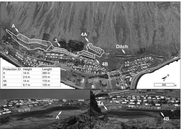
Table III. Analysis and uncertainty values for slope angle values plotted on profiles in Figure 6
Debris flow subareas ID 2013 2007 Median slope Mean slope Standard Deviation Median slope Mean slope Standard Deviation 1DFa 36.91 35.98 ±10 37.29 35.33 ±8 1DFb 37.96 38 ±7 48.83 49.44 ±8 1DFc 30.18 30.19 ±11 25.83 25.95 ±10 2DFa 38.08 37.61 ±7 44.21 43.83 ±13 2DFb 35.97 37.08 ±7 37.34 37.81 ±3 2DFc 32.57 31.15 ±7 30.73 32.4 ±12 11DFa 36.37 37.52 ±5 37.58 40.43 ±10 11DFb 33.85 33.74 ±2 33.33 33.24 ±2 12DFa 34.31 40.86 ±7 37.1 40.22 ±9 12DFb 34.31 34.48 ±2 34.65 34.46 ±2
Figure 7. (A) Elevation-difference map of debris-flow tracks 11DF and 12DF obtained calculating the difference in elevation between 2007 and 2013, overlying the hillshade model derived from 2013 LiDAR. (B) Maps of the erosion and deposition volume distribution of debris-flow tracks 11DF and 12DF derived by differencing the LiDAR gener-ated topography from 2007 and 2013. The debris flows were seg-mented in subareas of prevailing erosion and deposition along their length. [Colour figure can be viewed at wileyonlinelibrary.com]
11DFb and 12DFb: these subareas (Figure 7(B)) show zones of positive elevation change (up to 1 m), and these take the form of slightly outlined lateral levees and a straight terminal lobe (Figure 7(A)). These depositional landforms constitute 269 ± 10 m3 of material in 11DFb and 188 ± 13 m3 in 12DFb. The slopes along the steepest profiles of 11DFb and 12DFb show a steady trend with high average values (33°– 34°) in both years (Figures 6(J), (L), (N), Table III).
Discussion
Analysis of debris-flow initiation: 11DF and 12DF
A debris flow originates by slope failure when individual fail-ures, or numerous small failfail-ures, coalesce, transforming into a debris flow (Fairchild, 1987; Rodolfo et al., 1996; Iverson, 1997). Slope failure-initiated debris flows require the availabil-ity of loose material on steep slopes and an accumulation of wa-ter in the deposits, so they occur when rainfall and snowmelt cause an increase of pore-water pressures (Sidle and Swanston, 1982; Anderson and Sitar, 1995). This can commonly cause the rise of a water table at the contact of the debris cover with the impermeable bedrock or on top of impermeable layers (Camp-bell, 1975; Iverson, 1997; Decaulne et al., 2005). In the Westfjords of Iceland, long-duration rainfall and/or snowmelt associated with rain are the two main sources of water for trig-gering debris flows. For example, extreme rainfall of 63 mm/24 h after 1 month of rainy days (about 140 mm of cu-mulative precipitation) triggered the debris-flow event in Ísafjörður in September 1996 (Decaulne and Sæmundsson, 2007). Over 40 mm of one month-cumulative precipitation re-lated to snowmelt triggered a debris-flow event in Ísafjörður in June 1999, after a sudden (2 weeks) increase in air temperature from 1 to 4°C to 14–17°C (Decaulne et al., 2005; Decaulne and Sæmundsson, 2007). In Decaulne et al. (2005), the initiation for the debris-flow events in Ísafjörður in June 1999 is identified by the appearance of the subsurface runoff at the edge of the Gleiðarhjalli bench, causing erosion of material and generation of rotational slide evolving into debris flows downslope. Debris flows 11DF and 12DF— that were not present at the time of ob-servations made by Decaulne et al. (2005)— have these char-acteristics. Springs coming out between the sediment mantle and the bedrock are visible in aerial images in the scarp of 11DF (Figure 4(D), (F)), showing that runoff could have initiated erosional processes. This is a condition that has been observed in other environments; Bremer and Sass (2012) in the Austrian Alps identified the starting zones of debris flows at the bedrock–debris interface where runoff is concentrated. The combination of springs and loose debris has also been reported in the Alpine environment as one of the most important prepara-tory factors for slope failure (Marchi et al., 2002; Wieczorek and Glade, 2005). This is a plausible mechanism in Ísafjörður for the weakening and saturation of the deposits, leading to the devel-opment of discrete slope failures evolving into debris flows.
Debris flows 11DF and 12DF have a simple morphology: erosion in the upper part (11DFa with 832 ±31 m3, and 12DFa with 549 ± 24 m3) and deposition in the terminal part
(11DFb with 268 ±10 m3, and 12DFb with 188 ± 13 m3). Ero-sion extends from the edge of the bench, to the chutes, into the newly formed channels on the hillslope. Simple curved main scarps and crown-parallel tension cracks are due to a ro-tational sliding process (Figures 4(C)–(F), 8(A)). A negative ele-vation change of up to 5 m in the chute and in the channel shows that, once slope failure started from the front of the bench, it mobilised material that was already in transfer, and with saturation evolved into a debris flow, forming a terminal
lobe and lateral levees. Sediment transfer is further evidenced by the fact that in the chutes and upper channels, low slope values in 2007 match increased slope angles in 2013, and vice versa. The entrainment and transport of debris from the chutes and channels is also expected because of their gradient above 35° both in 2007 and 2013. Debris-flow tracks 11DF and 12DF are short:<250 m long.
Our suite of observations and measurements for 11DF and 12DF tracks fits with the characteristics of the slope failure pro-cess reported in the literature. Theule et al. (2012) used multi-temporal topographic surveying from TLS and ALS to monitor sediment transport by two debris flows in the French Alps. Low rainfall intensity events caused short-runout debris flows (less than 100 m) generated by talus slope failure (magnitude of erosion 266 m3, magnitude of deposition 268 m3). Cannon et al. (2001) reported ~84 debris flows in Colorado initiated by landslides; they back-traced the debris-flow paths to discrete landslide-scar sources and estimated their volumes, which had a range of ~95 to 2500 m3. Debris flows in Switzerland have been shown to originate from individual shallow rotational slides on slopes with angles between 25° and 45°, and with volumes of tens to a few hundred cubic metres (Hürlimann et al., 2003). The order of magnitude of the volumes and the size and morphological characteristics of the debris flows analysed in these three studies match well with our quantifica-tion and observaquantifica-tions of debris-flow tracks 11DF and 12DF (Figure 8(A)).
Analysis of debris-flow initiation: 1DF and 2DF
Material released by slope failure can be transferred into a channelised area. Then, debris can either be transferred down-slope, if saturated, evolving into a debris flow, or can cease to be mobile, generating a debris dam and obstructing the chan-nel (Bovis and Jones, 1992; Iverson et al., 2000). Formation of such a debris dam creates the optimal conditions for the devel-opment of the fire-hose effect. This mechanism occurs when an overland flow is concentrated by chutes or depressions in the bedrock and becomes a debris flow when impinging on loose debris accumulated in those depressions (Fryxell and Horberg, 1943; Curry, 1966; Johnson and Rodine, 1984; Berti et al., 1999; Coe et al., 1997, 2008; Glancy and Bell, 2000; Berti and Simoni, 2005; Larsen et al., 2006; Godt and Coe, 2007). Coe et al. (2008) reported that the initiation via the fire-hose ef-fect is controlled by the sediment supply, rather than by the moisture level.
In the Westfjords, Decaulne and Sæmundsson (2006) link the presence of release scars to debris flows originated by rotational slides. In Ísafjörður, debris-flow tracks 1DF and 2DF– not of new formation as 11DF and 12DF, but already formed at the time of the surveys– have curved release scarps showing signs of regressive erosion, ephemeral springs at the contact between loose debris and bedrock, erosion in the upper catchment (sub-areas 1DFa and 2DFa), and a main depositional area in the chute (subareas 1DFb and 2DFb). These are all evidence of slope failure, which through rotational sliding eroded material in the upper catchments and dammed the chutes depositing up to 3000 m3of debris at high slope angles (>35°). The slope failure process in this case has generated the preparatory condi-tions for future debris flows to occur. It is improbable that the de-posits currently located in the chutes remain stable.
In particular, we believe that the debris-flow tracks 1DF and 2DF show the preparatory conditions for the fire-hose effect. 54.7% and 81.3%, respectively, of the overall deposited vol-umes in 1DF and 2DF are gathered in the chutes. It has been observed that hundreds to a few thousand cubic metres of loose
deposits reflects pulses of sediment supply from upslope catch-ments (Theule et al., 2015), and that these pulses can be in-duced and fed by processes such as rockfalls (Loye et al., 2016). Cascades of processes leading to slope failure have been observed in the field and in experiments, where surface water runoff causes erosion and accumulation of material, sub-sequently mobilised by shallow slides. Depending on the to-pography, sediment can be re-accumulated and periodically released as a debris-flow surge when impinged on by water flow (Kean et al., 2013; Hu et al., 2016).
Debris flows can be initiated by saturation and breaching of dams of sediment located in channels. We suggest that 1DF and 2DF tracks show a favourable setting to the fire-hose effect, since scarp failure and sediment storage are present in the chutes and channels. We hypothesise that some of the accumu-lated debris has probably already been transported downslope by the fire-hose effect. This is suggested by a trend of alternat-ing zones of erosion and deposition throughout the 1DF and 2DF tracks and at different scales in the different subareas (Fig-ure 8(B)). For example, in the lower parts (1DFc and 2DFc) of debris-flow tracks 1DF and 2DF, small zones of deposition and erosion are aligned within the channel, and along the cen-tral steepest path in the upper catchments and apical chutes, particularly clearly in 1DFa (Figures 4(B), 5(B)). We infer that this setting cannot be due to the failure of pre-existing material, such the collapse of lateral levees or lateral banks (Frank et al., 2015; Hu et al., 2016), as in the DoD, erosion of these features would be visible in correspondence with deposition in the
chute or the channel. Therefore, we interpret these alternating zones of erosion and deposition to be likely the result of the transport of debris by the fire-hose effect: this has caused in-stantaneous sediment entrainment, as the build-up of the lateral levees occurs in association with discrete erosion zones in the chutes and channels (potential impact points; Coe et al., 2008). The presence of these fire-hose events is also supported by the erosion volume being larger than the deposited one (i.e. debris has left the survey zone).
In Table IV, we compare our volume calculations with the volume results obtained by Decaulne et al. (2005) and Conway et al. (2010). Our deposition results for 1DF (4079 ± 223 m3)
and 2DF (3760 ± 127 m3) are similar to those of Conway et al. (2010): 8287 m3and 1925 m3, respectively, for the same
tracks. The deposition value calculated for debris flow 2DF by Decaulne et al. (2005) matches fairly well with our calcula-tion, but the event described by these authors extended to the base of the slope. In our study, much of the total deposited vol-umes for 1DF and 2DF lies in the chutes (1DFb with 2234 ± 21 m3and 2DFb with 3058 ± 30 m3in Table IV), rather than
along the tracks, or in the depositional lobes as measured by Decaulne et al. (2005) and Conway et al. (2010). These vol-umes are of the same order of magnitude as the material mobilised by a debris flow in 1999 (estimated at 3000 m3for 2DF; Decaulne et al., 2005) and from 1999 to 2007 (1925 m3 for 2DF; Conway et al., 2010). Previous studies (Glade, 2005; Decaulne and Sæmundsson, 2006; Conway et al., 2010) recognised debris flows that had originated through the
fire-Figure 8. Simplified sketch of the main geomorphological characteristics of the slope failure (A) and the fire-hose effect (B). [Colour figure can be viewed at wileyonlinelibrary.com]
hose effect in other areas of the Westfjords in Iceland, but with a lower frequency (~10 years return) than the mean return pe-riod of Gleiðarhjalli area (4–5 years; Decaulne et al., 2005). Those previous studies considered the fire-hose effect to only involve smaller volumes of material (700–1000 m3), based on debris collected in the chutes by weathering and erosion of the bedrock (i.e. those flows are most likely supply-limited). Since 2007, much larger volumes gathered in the chutes of 1DF and 2DF tracks (subareas‘b’) at high slope angle (~37– 38°, see Figure 6). This setting is vulnerable to the fire-hose ef-fect, and shows high potential mobility of the debris in the chutes of the 1DF and 2DF tracks.
Summary of debris-flow initiation processes
identified in Ísafjörður
We have shown that the use of differenced LiDAR datasets for volume change detection, integrated with slope and geomor-phic analysis from remote sensing data, and demonstrate its potential for identifying debris-flow initiation processes. The deposits in the chutes described by us would be‘invisible’ in the datasets of Conway et al. (2010) and Decaulne et al. (2005), since in their field-based studies they could not quantify the material in the chutes of the flows. Our approach of identi-fying pre- and post-events changes in topography, volumes, slopes and morphology allowed us to distinguish between the slope failure initiation process and the formation of preparatory conditions for the fire-hose effect without having to witness them, making possible a discrimination that would have been virtually impossible otherwise.
The slope failure and the fire-hose effect as initiating processes for debris flows in the Westfjords were previously only hypothesised (Decaulne et al., 2005; Decaulne and Sæmundsson, 2006; Conway et al., 2010). The comparison of air-borne datasets with a 6-year separation shows that the four debris-flow tracks analysed are geomorphically distinctive (see Figure 8) and show two different modes of flow initiation and evolution: (1) Slope failure is the mechanism that triggered the
newly-developed debris flow 11DF and 12DF, and that caused erosion in the upper catchments and deposit transfer in the chutes of the already-formed 1DF and 2DF tracks. (2) We have been able to quantify the magnitudes of the
vol-umes of material stored within debris-flow chutes and tracks above Ísafjörður by slope failure: this has produced debris dams at high slope angle, forming the preparatory conditions for the fire-hose effect. Part of this debris has probably already been transported by this mechanism. The large volumes of material stored in the chutes and channels of 1DF and 2DF (2000–3000 m3 in subareas 1DFb and 2DFb) in the past were probably moved in a sin-gle sudden event, so they provide a substantial amount of material that could be mobilised by the fire-hose effect, leading to potentially hazardous debris flows, as cyclic damming has been proved to enlarge the size of new debris-flow pulses (Hu et al., 2016). This further suggests that this repeated storage of large volumes of sediment in the upper parts of the slope could result in longer runout debris-flow tracks, compared to smaller flows that are formed by single slope failures.
Implications for potential mobility and hazard
In general, slope angles exceeding 20°–40° are sufficient for the development of slides in dry conditions, and these values can
Table IV . Data re garding the debri s flo ws descri bed in th is study , com pared with th e data of Conw ay et al . (2010) and Decau lne et al . (2005) De bris flow ID Y ears of ac tivity Y e a rs o f data collec tion s and auth ors Metho d o f survey Estimated deposit ion m 3 (stan dard er ror) Depo sition m 3 (rela tive uncerta inty) -Thi s stud y Estimated er osion m 3 (stan dard error ) Ero sion m 3 (rela tive unc ertai nty) -Thi s stud y 1DF June 2006, 200 7-2013 Summe r 2007 , Sum mer 2008: C onwa y e t al. (20 10) LiDAR/airbo rne photog rap hs, DGP S 8000 (±6 6%) _ 41000 (±3 8%) _ Summe r 2007 , Sum mer 2013: Thi s stud y LiDAR/airbo rne photog rap h _ 4079 (±5%) _ -8552 (±4% ) 2DF 1965, June 199 9, Ju ne 2006, 2007-2013 Summe r 1999 : D e caulne et al. (2 005) Aerial photo graphs, field survey 3000 _ _ _ Summe r 2007 , Sum mer 2008: C onwa y e t al. (20 10) LiDAR/airbo rne photog rap hs, DGP S 2000 (±13 4%) _ 16000 (±6 2%) _ Summe r 2007 , Sum mer 2013: Thi s stud y LiDAR/airbo rne photog rap hs _ 3760 (±3%) _ -5000 (±4% ) 1 1DF 2007-2013 Summe r 2007 , Sum mer 2013: Thi s stud y LiDAR/airbo rne photog rap hs _ 339 (±9%) _ -862 (±5% ) 12DF 2007-2013 Summe r 2007 , Sum mer 2013: Thi s stud y LiDAR/airbo rne photog rap hs _ 271 (±1 1%) _ -628 (±7% )
be much lower in saturated conditions, depending on the na-ture of the material (Anderson and Anderson, 2010). Mean values of slope angles in 2013 in the upper zones of all the analysed debris flows are high (Table III; 36° in 1DFa, 38° in 2DFa, 37° in 11DFa, 41° in 12DFa). Instead of decreasing since 2007, the slope angle in the scarp zones is maintained, hence prone to new slides. We also found such high angles in other debris-flow chutes along the slope above Ísafjörður (Figure 9). Over an area of 0.55 km2defined along the edge of the bench, we calculated that ~17% is occupied by deposits perched on slopes exceeding 35° and ~4% exceeding 45°. This means that all these areas could be prone to failures.
In geomorphologic studies, the mobility of gravitational movements has been related to the volume and angle of repose (Corominas, 1996; Rickenmann, 1999; Legros, 2002; Toyos et al., 2008). Steep slopes and initial failure volume have previ-ously been shown to be important factors with respect to debris-flow initiation (Bovis and Dagg, 1992; Iverson, 1997; Brayshaw and Hassan, 2009). Steep channels are intrinsically less stable than low-angle channels, thus debris-flow initiation is more likely. In addition, large sediment volumes – which can self-increase as they travel downslope if runoff-initiated, as with fire-hose or sediment bulking (Godt and Coe, 2007)– usually travel at a higher flow speed than small failures when they enter the channel. Large volumes acquiring high speed
are also more likely to impinge catastrophically on saturated deposits stored in the channel, triggering a further debris flow. Furthermore, the incision of the channel can progressively in-crease the volume of the flow during different debris-flow surges, with further material supplied in the flow by processes like channel scouring (Rickenmann and Zimmermann, 1993; Berti et al., 1999; Hungr et al., 2005). For these reasons, deeply incised pre-existing tracks like 1DF and 2DF in Ísafjörður are a further source of instability for the material upslope, and consti-tute a preferential path for sediment delivery downstream.
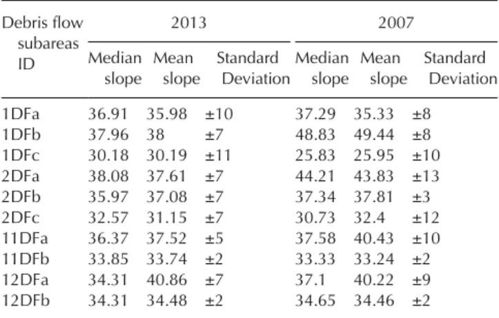
A high mobility debris flow, such as those that could be ini-tiated by the fire-hose mechanism in tracks 1DF and 2DF, poses a potential hazard to people and property. The construction of new engineering solutions (in Figure 10 barriers A, 4A and 4B realised with gabions) and the improvement of old ones (barrier 3) to protect Ísafjörður from debris flows and snow avalanches were commissioned in 2012 (Municipality of Ísafjörður; report in Icelandic) and constitute a substantial improvement to the risk mitigation of the town. Old barrier 3 has been raised from 3 m to 5 m, while the new ones reach heights of up to 14 m. As barriers A and 3 are positioned beneath debris flow 2DF, they have the potential to retain a new flow in this track. How-ever, there is no protection apart from the ditch beneath debris flow 1DF, whose terminal lobe deposits are located just 90 m above the main road (Figure 10).
Figure 9. Slope map calculated from DEM 2013, showing loose deposits with angle higher than 35° and 45°. [Colour figure can be viewed at wileyonlinelibrary.com]
Figure 10. Plan of the snow avalanche and debris-flow protection measures ordered by the municipality of Ísafjörður in 2011 (protection measures have the same naming protocol used in the report in Icelandic from the municipality). Ditch and barrier 3 were already present in 2013 (ditch 2–3 m deep, barrier 3 3 m high). Dashed red line marks the perimeter of studied debris flows. [Colour figure can be viewed at wileyonlinelibrary.com]
The presence of these engineering solutions suggests that previous studies contributed to planning the measures of haz-ard mitigation for the town of Ísafjörður. Further efforts should be made in understanding debris-flow initiation, as the reliance of runout distance, flow volume, and return period for debris flows on their initial triggering mechanisms has broad implica-tions for assessment of debris-flow hazards.
Finally, we note that the high quality topography data that can be obtained from airborne LiDAR surveys can be effec-tively used for hazard-monitoring purposes, but they are expen-sive and time-consuming to process. In this perspective, the use of unmanned aerial systems (UAS) able to collect topography data (usually from photogrammetry) and remote sensing images has been proven a valuable resource for high-resolution hazard surveys (Mancini et al., 2013; Lucieer et al., 2014; Jordan and Napier, 2015), and could be used as a data source for the same kind of analyses that we describe here. Annual UAS surveys of the debris-flow tracks above Ísafjörður could provide a flexible, cost-effective, and time efficient method for monitoring their evolution, especially the build-up of deposits in unstable parts of long tracks located above inhabited areas. Such data would also provide an important scientific resource for furthering the study of debris-flow initiation and evolution.
Conclusions
We have compared two airborne datasets (LiDAR topography and aerial images), collected in 2007 and 2013, that describe debris flows above the town of Ísafjörður in Iceland. This multi-temporal high-resolution approach reveals details about debris-flow processes in the steepest source areas that previous studies using traditional survey techniques (Decaulne et al., 2005; Conway et al., 2010) were unable to fully analyse. Our main conclusions are:
(a) Slope failure of the deposits from the edge of the Gleiðarhjalli bench is the dominant initiation process, lead-ing to a new generation of debris-flow landforms above the town (11DF and 12DF) and mobilising debris now in transit in the chutes and upper channels of pre-existing tracks (1DF and 2DF). The fire-hose effect could re-activate older flows (1DF and 2DF), and has probably already mobilised debris within their channels.
(b) The two mechanisms can be geomorphologically distin-guished, with slope failure characterised by a simple upper–lower erosion–deposition pattern, defined scarps with possible regressive erosion, steep (>35°) discrete slide surfaces with ephemeral springs, modest (below 1000 m3) mobilised volumes, and short-runout. Preparatory condi-tions for the fire-hose effect-triggered debris flows are dis-crete zones of deposited material at high angle (>35°) in the chute and along the channel, and alternating zones of fill and scour along their whole length.
(c) Volumes of debris stored in the chutes and upper channels of medium-scale debris-flow tracks 1DF and 2DF (2200– 3000 m3) are stored at high angles (37–38°) and have the same order of magnitude as those estimated for single dam-aging events that happened in the past (Decaulne et al., 2005; Conway et al., 2010). We infer that these two debris dams have high potential mobility. This confirms hypothe-ses previously suggested (but not confirmed directly, nor precisely quantified) by Decaulne et al. (2005) and Con-way et al. (2010)– namely that there are large volumes of material blocking steep channels in Ísafjörður.
More widely, we have shown that our geomorphic criteria ap-plied on LiDAR differencing has permitted us to detect, quantify
and characterise debris accumulated at high gradients, without the assistance of any other monitoring system or information on the evolution of the debris flow and of their triggering condi-tions. The slope of Ísafjörður is extremely prone to activation and re-activation of debris flows, so this kind of study in this and other debris-flow threatened areas, supported by in situ channel survey and monitoring, can improve our understand-ing of both how debris flows develop and how to mitigate the risks associated with them.
Acknowledgements—This work would not have been possible without a postgraduate studentship grant (NE/L002493/1) from the CENTA Doc-toral Training Partnership funded by the UK Natural Environment Re-search Council (NERC) and the British Geological Survey University Funding Initiative Studentship (GA/14S/024, Ref: 284). We thank the NERC Airborne Research Facility Data Analysis Node for obtaining the aerial photography and LiDAR data, for the airborne survey project NERC ARSF 07217a in 2007 and for the airborne survey project NERC ARSF IG13-11 in 2013. We thank the NERC Geophysical Equipment Facility for technical support and for the loan number 1001. We would like to show our gratitude to Jón Kristinn Helgason (Icelandic Meteoro-logical Office), who provided expertise that greatly improved the man-uscript. We acknowledge constructive comments and suggestions from two anonymous reviewers. C. Jordan publishes with permission from the Executive Director of the British Geological Survey.
Conflict of Interest
The authors declare no competing interests.
References
Akca D. 2007. Least Squares 3D Surface Matching. Zurich: Eidgenössische Technische Hochschule Zürich.
Anderson RS, Anderson SP. 2010. Geomorphology: the Mechanics and Chemistry of Landscapes. Cambridge University Press: Cambridge. Anderson SA, Sitar N. 1995. Analysis of rainfall-induced debris flows.
Journal of Geotechnical Engineering121: 544–552. https://doi.org/ 10.1061/(ASCE)0733-9410(1995)121:7(544).
Bangen S, Hensleish J, McHugh P, Wheaton J. 2016. Error modeling of DEMs from topographic surveys of rivers using fuzzy inference sys-tems. Water Resources Research 52: 1176–1193. https://doi.org/ 10.1002/2014WR015716.
Berti M, Genevois R, Simoni A, Tecca PR. 1999. Field observations of a debris flow event in the Dolomites. Geomorphology29: 265–274. https://doi.org/10.1016/S0169-555X(99)00018-5.
Berti M, Simoni A. 2005. Experimental evidences and numerical modelling of debris flow initiated by channel runoff. Landslides2: 171–182. https://doi.org/10.1007/s10346-005-0062-4.
Besl P, McKay N. 1992. A method for registration of 3-D shapes. IEEE Transactions on Pattern Analysis and Machine Intelligence 14: 239–256. https://doi.org/10.1109/34.121791.
Blasone G, Cavalli M, Marchi L, Cazorzi F. 2014. Monitoring sediment source areas in a debris-flow catchment using terrestrial laser scanning. Catena 123: 23–36. https://doi.org/10.1016/j. catena.2014.07.001.
Bossi G, Cavalli M, Crema S, Frigerio S, Quan Luna B, Mantovani M, Marcato G, Schenato L, Pasuto A. 2015. Multi-temporal LiDAR-DTMs as a tool for modelling a complex landslide: a case study in the Rotolon catchment (eastern Italian Alps). Natural Hazards and Earth System Sciences15: 715–722. https://doi.org/10.5194/nhess-15-715-2015.
Bovis M, Jones P. 1992. Holocene history of earthflow mass movements in south-central British Columbia: the influence of hydroclimatic changes. Canadian Journal of Earth Sciences29: 1746–1755. Bovis MJ, Dagg BR. 1992. Debris flow triggering by impulsive loading:
mechanical modelling and case studies. Canadian Geotechnical Journal29: 345–352.
Brasington J, Langham J, Rumsby B. 2003. Methodological sensitivity of morphometric estimates of coarse fluvial sediment transport.