HAL Id: hal-00280400
https://hal.archives-ouvertes.fr/hal-00280400v2
Submitted on 3 Jun 2016
HAL is a multi-disciplinary open access
archive for the deposit and dissemination of
sci-entific research documents, whether they are
pub-lished or not. The documents may come from
teaching and research institutions in France or
abroad, or from public or private research centers.
L’archive ouverte pluridisciplinaire HAL, est
destinée au dépôt et à la diffusion de documents
scientifiques de niveau recherche, publiés ou non,
émanant des établissements d’enseignement et de
recherche français ou étrangers, des laboratoires
publics ou privés.
A Multiple Description Coding strategy for Multi-Path
in Mobile Ad hoc Networks
Eddy Cizeron, Salima Hamma
To cite this version:
Eddy Cizeron, Salima Hamma. A Multiple Description Coding strategy for Multi-Path in Mobile Ad
hoc Networks. ICLAN 2007, Nov 2007, Paris, France. pp.39-44. �hal-00280400v2�
A Multiple Description Coding strategy for
Multi-Path in Mobile Ad hoc Networks
Eddy Cizeron
Institut de Recherche en Communications et en Cybern´etique de Nantes Rue Christian Pauc BP 50609 44306 Nantes cedex 3 France Email: [email protected]
Salima Hamma
Institut de Recherche en Communications et en Cybern´etique de Nantes Rue Christian Pauc BP 50609 44306 Nantes cedex 3 France Email: [email protected]
Abstract—One of the main challenges for mobile ad hoc
networks is to design routing protocols that cope efficiently with dynamic network topologies. In this paper, we propose a routing strategy in a multipath context and adapted to proactive protocols like OLSR. The main idea is to use the sizeable amount of information collected by every node in order to select not one but several reliable routes used simultaneously. Then, the information is not merely parcelled out between these routes, but coded using a Multiple Description method, which reduces the dependency on topology changes. Each route among the N selected ones is used to transmit a specific description. Any subset of M routes among these N routes is sufficient to rebuild the initial data information. Furthermore, thanks to path diversity, the local bitrate is reduced. This feature may be interesting in the case of multimedia information exchanges (such as video) over mobile ad hoc networks. Performance analysis of this new algorithm shows that the paths reliability is improved. In particular, load balancing for high bitrates and dense networks enables to reach interesting performances.
I. INTRODUCTION
A Mobile Ad hoc NETwork (MANET) is a collection of mobile wireless devices. The main characteristic of such a network is the perpetual change of topology due to mobility, appearance and disappearance of the nodes. For each pair of nodes in the network that have to communicate, the routing protocol must ensure the construction and the maintenance of at least one muti-hop path. In this context, certifying the stability of the transfer (by maintaining a constant delay and limiting retransmission) is a highly challenging issue.
Among the large amount of already existing protocols, a usual categorization discriminates reactive and proactive ones. In reactive protocols, routes are built on demand while in proactive protocols, recurring updates ensure that a path to every destination is determined a priori. In this paper, we will focus on proactive protocols and particularly on Optimized
Link State Routing protocol (OLSR) [2]. We propose an
improvement of OLSR route selection process and a new organisation of data transmissions. We call MP-OLSR this OLSR-like protocol.
The remainder of this paper is organized as follows: in sec-tion 2, we present other multi-path routing protocols proposed in literature. In section 3, we briefly introduce the principle of the multiple description coding and its practical application
using multiple routes discovered. The path selection algorithm is then described in section 4. The main hypotheses and metrics are given in the same section, as well as the description of the functions used as parameters of our algorithm. Section 5 gives the simulation results, focusing on the reliability criterium, and their analysis. Eventually, section 6 concludes our paper and presents outlooks.
II. MULTI-PATHROUTINGPROTOCOLS
A usual method proposed in literature consists in using only one route among the determined ones. In case of transmission failure, it is replaced almost instantaneously by an alternate route. The Split Multi-path Routing protocol (SMR) proposed in [3] focuses on the selection of multiple routes of maximally disjoint paths to prevent certain nodes from being congested but distribute information in only two routes per session.
The Multi-path Dynamic Source Routing protocol (MP-DSR) defines a new QoS metric, end-to-end reliability in order to select a subset of end-to-end paths to provide increased stability and reliability of routes [3]. In [5] The On Demand
Multi-path routing builds multiple routes but uses only the
primary route while alternate routes are used only when the primary one fails.
Other solutions are based on an optimal method [8] such as in [6]. The authors build completety disjoint routes (i.e. disjoint by nodes and links) which limited the number of routes. In [1] authors proposed shortest paths (i.e. minimum number of hops) with fewer number of disjoint nodes between two paths. Consequently, such algorithms are not appropriate for multiple description coding purpose.
III. THEMULTIPLEDESCRIPTIONCODINGAPPROACH
Multiple Description Coding (MDC) refers to a group of data representation and transformation methods which pur-pose is to improve the transmitted information integrity by transforming it into a set of redundant data packets called descriptions.
A. MDC principle
Given a piece of information I, a multiple description coding method generates N independently communicable
packets (D1, D2, ..., DN). Each description Di is generally
much smaller than the original information. However, the total size of all descriptions is higher than the size of the original message I. This set of descriptions is such that there exists an integer M (0 ≤ M ≤ N ) such that every subset of descriptions containing at least M different descriptions is sufficient to rebuild I. Thus, the higher is M , the lower is the redundancy. In particular, M = 1 (respectively M = N ) corresponds to
the case where (Di)i∈[1,N ]are copies of I (respectively where
(Di)i∈[1,N ] are different pieces of I). For a detailed review,
refer to [7].
B. MDC, OLSR and MP-OLSR
The operation of OLSR, as in every proactive link-state rout-ing protocol, consists in two main steps: topology discovery and computation of the shortest path in order to determine the most appropriate next hop for every potential destination. In the first step, each node floods the network with a packet that contains its neighborhood information. This information, collected by all the other nodes, allows them to build a virtual representation of the actual network topology. A shortest path algorithm (generally Dijkstra’s algorithm) provides the best path to reach each destination. In fact, for a given destination, only the next node of the path is recorded. No global view of paths is considered: an intermediate node of a given communication only supervises the next hop. In the proposed approach, several routes are determined for a given destination. One major difference with OLSR strategy is that routes are not selected repeatedly after every flooding procedure, but only when a destination has to be reached. Furthermore, the source
entirely determines the routes. For each route, a description Di
is then generated and sent. By propagating through redundant paths, information is less influenced by route failures. Even if a certain number of the N paths vanishes, if at least M are valid, the communication can go on.
IV. ROUTE SELECTION ALGORITHM
The aim of this procedure is to build a set K of N paths, with no loops, joining a source node (noted s) and a destination node (noted d). This set must comply with the following conditions: the number of elements (nodes and links) shared by two distinct routes of K is as small as possible; the cost of each route of K is as small as possible. It appears that these two properties cannot be perfectly satisfied at the same time.
A. Hypotheses
An ad hoc network is represented by a graph G = (V, E, c) where V is the set of vertices, E ⊂ V × V the set of arcs and
c : V → R∗+ a strictly positive cost function. We assume the
graph is initially undirected (i.e. (v1, v2) ∈ E ⇒ (v2, v1) ∈ E
and c(v1, v2) = c(v2, v1)) and loopless (i.e. no arcs joining
a node to itself). We also assume that any pair of vertices cannot be connected by more than one arc. Given an ordered pair of distinct vertices (s, d) we can define a path between
s and d as a sequence of vertices (v1, v2, ..., vm) such that
(vq, vq+1) ∈ E , v1= s and vm= d.
B. Path selection metric
The above representation implies that we define precisely what the cost function c refers to in an ad hoc context. Generally the cost of a link is an quantitative assessment of its quality. The cost is additive and as small as the link is considered good. For example, it can be the delay necessary to deliver information through it, a quantity based on the bit error rate, or on the dependency on interferences.
Considering the period T between too successive updates
for the same link e, we define πeas the probability that the link
e is actually able to transmit the data during T . Of course πe
depends on the physical properties of the environnement, but it also reckons with the vertices mobility and the local stability of the neigbourhood relation. One possible way of evaluating this value could be to use statistical properties of the periodic
control messages. c is then defined as c(e) = − log(πe). This
information has to be transmitted along with the neighborhood during the flooding procedure as OLSR allows it.
One can notice that the chosen metric, is not only correlated with the physical quality of links (such as mean delay, binary error ratio or more complex metrics as in [9]) but also with its limited livespan, due to topology changes.
C. Proposed algorithm
Let fp : R∗+ → R∗+ and fe : R∗+ → R∗+ be two
functions such that id < fpand id ≤ fe< fp(where id is the
identity function). The proposed algorithm (see 1) is applied
to a graph G = (V, E, c), two vertices (s, d) ∈ E2and a strictly
positive integer N . It provides a N -uple (P1, P2, ..., PN) of
(s, d)-paths extracted from G.
M ultiP athDijkstra(s, d, G, N )
c1← c
G1← G
for i ← 1 to N do
SourceT reei← Dijkstra(Gi, s)
Pi ← GetP ath(SourceT reei, d)
for all arcs e in E do
if e is in Pi OR Reverse(e) is in Pi then
ci+1(e) ← fp(ci(e))
else if the vertex Head(e) is in Pi then
ci+1(e) ← fe(ci(e))
else
ci+1(e) ← ci(e)
end if end for
Gi+1← (V, E, ci+1)
end for
return (P1, P2, ..., PN)
Algorithm 1. Calculate N routes in G from s to d
where Dijkstra(G, n) is the standard Dijkstra’s algorithm which provides the source tree of shortest paths from vertex n in graph G; GetP ath(SourceT ree, n) is the function that ex-tracts the shortest-path to n from the source tree SourceT ree;
Reverse(e) gives the opposite edge of e; Head(e) provides the vertex edge e points to.
D. Incrementation Functions
The cost incrementation functions fp and fe are used
at each step in order to prevent Dijkstra’s algorithm from generating a new path between s and d that would be too similar to one already found. This way, they ensure a certain diversity in the final N -tuple, but contrary to what provide most of multi-path computation algorithms, generated paths need not be completely disjoint. This choice is due to several considerations explained below.
First, the number of disjoint paths is limited to the (s, d) minimal cut (defined as the size of smallest subset of edges one cannot avoid in order to connect s and d). This minimal cut is often determined by the source and destination neighborhoods. For example, if s only has 3 distinct neighbors, one cannot generate more than 3 disjoint paths from s to d. As a consequence, this limitation of diversity may be local, the rest of the network being wide enough to provide far more than 3 disjoint paths. Another drawback of completely disjoint paths algorithms is that it may generate very long paths as every local “cutoff” can only be used once.
Secondly, we don’t focus in this paper on the optimal solution. Generally, optimal algorithm (as in [8]) provides a set of disjoint paths whose global cost (sum of all path costs) is
minimal. In our case, adding the cost c(e1) + c(e2) of
succes-sive arcs e1 and e2 is equivalent to multiplying their success
probabilities and thus to consider the success probability of their concatenation. In the same manner, adding the costs of two parallel paths is equivalent to computing the probability that they both succeed. However, we do not expect the result to contain simultaneously valid paths, but enough valid paths among all paths generated. As a consequence, the interesting value is the probability that the valid number of routes during period T (between two updates) is at least a given threshold M , which is highly more difficult to maximise. Nevertheless, given that the real topology may be quite unstable, we expect a practical algorithm to be sufficient to quickly obtain interesting paths.
fp is used to increase costs of the arcs belonging to the
previously path Pi (or which opposite arcs belong to it). This
encourages future paths to use different arcs but not different
vertices. fe is used to increase costs of the arcs who lead to
vertices of the previous path Pi. As a consequence 3 possible
behaviors can be distinguished:
• if id = fe< fp, paths tend to be arc-disjoint;
• if id < fe= fp, paths tend to be vertex-disjoint (which
is stronger than the previous case);
• if id < fe< fp, paths also tend to be vertex-disjoint, but
when not possible they tend to be arc-disjoint.
E. Algorithmic complexity and improvements
Dijkstra’s algorithm performs generally in O(|V|2+ |E |)
(although complexity may be reduced in the case of sparse
graphs). Thus global complexity is O(k(|V|2+|E |)). However,
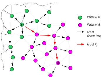
s d Vertex of Bi Vertex of Ai Arc of SourceTreei Arc of Pi
Fig. 1. Set of vertices to which Dijkstra must be re-applied at step i + 1
at each step i (1 ≤ i ≤ k) of our algorithm, Dijkstra’s algorithm has not to be applied again to all vertices. Given
path Pi let us consider Ai, the set of vertices that belongs to
the SourceT reei branch which contains Pi. Otherwise, node
v is in Ai if the shortest path from s to v in Gi shares at least
one arc with Pi. Let Bi = V \ Ai(see figure 1). We can easily
prove that for every vertex x in Bi, the shortest path from s to
x deduced from SourceT reei can still be used at step i + 1.
Proof : For v ∈ V let us call Pis→n the shortest path
from s to v in Gi. Pis→n is thus the shortest path from s
to v provided by SourceT reei. We can notice that if v ∈ Bi
then all vertices of Pis→v belong to Bi. Let us suppose that
for some x ∈ Bi, Pis→x 6= Pi+1s→x. Given an arc e, its cost
increases between step i and step i + 1 if and only if head(e)
is in Pi. Thus, all the more, only if head(e) is in Ai. As
every vertex of Ps→x
i is in Bi, the costs of arcs of Pis→x
remain the same in Gi+1: ci+1(Pis→x) = ci(Pis→x). The fact
path Ps→x
i+1 has been selected at step i + 1 implies that its
new cost is either smaller or equal to the constant cost of
Ps→x
i : ci+1(Pi+1s→x) ≤ ci+1(Pis→x) and thus smaller or equal
to its own previous cost: ci+1(Pi+1s→x) ≤ ci(Pi+1s→x). As those
transformations never reduce the costs of arcs, the cost of a path cannot decrease. As a consequence we can ensure that:
ci(Pi+1s→x) ≤ ci+1(Pi+1s→x). That proves that the cost of P
s→x i+1
is also constant and equal to the one of Rs→xi . This cost is
still minimal at step i + 1 and, as a consequence, we need not
compute any new path Pi+1s→x.
Moreover, as neighborhood information is received period-ically, we may also adapt selected routes. Let us suppose that
a last graph Gk+1 has been generated after the path Pk
com-putation. Receiving neighborhood information, we can deduce if one or more previously chosen paths have disappeared or
have become unreliable. In this case, we can modify Gk+1 by
giving back to all concerned arcs (those who points to these arcs) their previous costs and execute as many steps of the algorithm as we have paths to replace.
s
d
K '2= {P2}
K '1= {P1,P4}
K '3= {P3,P5}
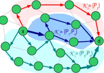
Fig. 2. Example of three subsets K01, K02 and K03
F. OLSR adaptation to multi-path context
The multi-path computation algorithm in mobile ad hoc net-work requires modification of the data circulation in compari-son with the classical OLSR protocol, in particular concerning the use of routes.
In OLSR protocol, each node maintains a routing table that contains the appropriate next node to use in order to reach any given destination. Our approach is a source routing strategy. This means that normally, every description packet must contain the path to follow as it has been defined by the source. Then intermediate nodes should not be allowed to disobey it. As a matter of fact, if they do so, the source may not be able to control the path dispersion anymore.
V. SIMULATIONS
A. Performance criteria: Reliability
Let us consider a set of N paths K = (P1, P2, ...PN) from
s to t. For every edge e we can define the random variable
Xeas being equal to 0 if the edge fails and to 1 if it is valid
during the period T between two consecutive updates for e. We consider that edges are independent. Similarly we can define
a random variable Yi for route Pi. We have Yi =Qe∈PiXe.
The random variable Z that provides the number of available
routes is equal to Z =P
iYi=Pi
Q
e∈PiXe. Supposing that
N descriptions (D1, ..., DN) have been generated from I (the
information to send), we use path Pi to carry Di. The ability
to reconstruct I at the destination is equal to the probability of receiving enough descriptions. Of course this depends on the parameter M used for multiple description coding.
For given values of M and N , we can define the reliability
ρ of K = (P1, P2, ...PN) as the probability that Z ≥ M . The
higher is ρ, the most probably the destination may obtain the information. The calculation of ρ requires to keep in mind that paths are not necessarly disjoint.
We can define sets K01, K20, ..., Kg0 following the definition:
each path of K must belong to exactly one set K0i; two paths
that share at least one arc must be in the same set Ki0; a set K0i
cannot be divided in two subsets with no common arcs. Figure 2 illustrates the distribution of 5 paths among 3 subsets.
We can then define the random variable Zj as the
number of available routes in K0j. Then, as (K0j)j are
edge-disjoint, (Zj)j are independent: P r(Z ≥ M ) =
P m1+...+mg≥M Qg j=1P r(Zj = mj). Calculating P r(Zj = 0 e in P1 πe = 0.74 e in P3 πe = 0.81 0 0 0 0 0 0 1 0 0 0 0.26 0 0 0 0.74 e in P1 and P2 πe = 0.73 0 0 0.05 0.21 0 0 0.14 0.60 0.05 0.22 0.04 0.15 0 0 0.10 0.44 e in P2 and P3 πe = 0.90 0.09 0.20 0.04 0.13 0.05 0 0.09 0.40 p' p represents p' = πe . p p' p p1 pi represents p' = p + (1 – πe ) . ( p1 + ... + pi )
Pr( Y1=0 & Y2=0 & Y3=0 )
Pr( Y1=0 & Y2=0 & Y3=1 )
Pr( Y1=0 & Y2=1 & Y3=0 )
Pr( Y1=0 & Y2=1 & Y3=1 )
Pr( Y1=1 & Y2=0 & Y3=0 )
Pr( Y1=1 & Y2=0 & Y3=1 )
Pr( Y1=1 & Y2=1 & Y3=0 )
Pr( Y1=1 & Y2=1 & Y3=1 )
Fig. 3. Example of the beginning of the computation of P r(Y1 = y1 &
Y2= y2& Y3= y3) for a subset K0= {P1, P2, P3}
m) requires to construct paths by considering successively
every edge e of K0j = {Pj1, ...Pjnj} and to consider the
values of P r(Yj1 = y1 & Yj2 = y2 & ... & Yjnj = ynj)
with y ∈ {0, 1}. At each step the probabilities of the different
cases are modified. If K0jcontains njpaths, there are 2nj cases
to process at each step (corresponding to all possible values of (y1, ..., ynj)).
Figure 3 shows the 4 first steps of the procedure used for a
subset K0= {P1, P2, P3}.
In our approach, vertices are considered entirely trustwor-thy. This hypothesis might be deemed as unrealistic but we consider that every vertex failure can be taken into account as the failure of all its edges.
B. Model description
Our simulations require to define ad hoc network topologies. This is done by spreading a given number of nodes in a square area. All nodes have the same range. A source and a destination are designated. Each link e is given a success
probability πe by randomly selecting a value in a given
subinterval of [0, 1]. Furthermore, we take into consideration the limited memory available at each intermediate node for messages. This implies a dependency between nodes and their received bitrates. As our calculation is based on links reliabilities, we multiply the success probability of every link
e by the coefficient 1 − exp(−Λ/λv) where Λ is a constant
and λvthe bitrate received at node v, the head of e. As packets
are transformed before being sent, the actual bitrate on a given path is smaller than the bitrate of transfer λ. We consider optimal multiple description coding, thus on every path P the
birate is λP = λ/M . If Uv is the number of paths using node
v, the bitrate on v is λv = λUv/M . Table I provides the
different parameters considered in the simulated scenarios.
C. Results analysis
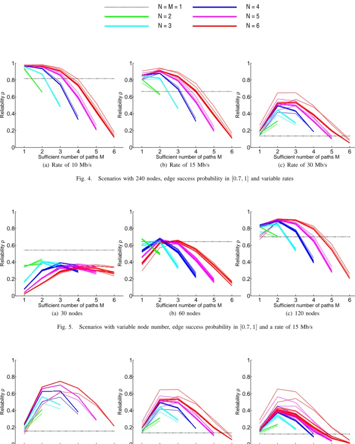
Figures 4, 5 and 6 represent the values of reliability ρ function of the parameter M . Colors refer to N , the total number of used routes (green for 2 routes, cyan for 3 routes, blue for 4 routes, purple for 5 routes and red for 6 routes). Different curves of a same color correspond to different kinds
Range of nodes 200 m Area dimension 1000 m × 1000 m Λ 60 Mb/s Number of nodes 30, 60, 120, 180 or 240 Edge success [0.9, 1], [0.7, 1] or [0.5, 1] probability Transfer rate λ 3 Mb/s, 6 Mb/s, 10 Mb/s, 15 Mb/s or 30 Mb/s fp fp(c) = c + c0 c0∈ {0.1, 0.3, 0.7, 1, 2, 5} fe id ≤ fe≤ fp Number of routes N 2, 3, 4, 5 or 6 Number of routes 1 ≤ M ≤ N necessary for reconstruction M TABLE I
PARAMETERS USED IN THE SIMULATED SCENARIOS
of incremental functions. The dotted horizontal line indicates the reliability of the best path used alone, which corresponds to the case where N = M = 1.
A general observation is that the choice of the incremental function is not so much relevant in comparison with the choice of other parameters. We remind that the cases where M = 1 and N > 1 correspond to the creation of N copies of the original data and the cases where M = N correspond to the division of the original data in N non-redundant parts. This strategy does not seem relevant because it requires all routes to be valid together. This surmise is confirmed by all the figures: the reliability becomes very low when M tends to N .
1) Influence of rate: In figure 4, it is noticeable that in case
of a low bitrate, we obtain very good values for low values of M . This can be explained by the fact that even if copies are created, as they are small, the transfer efficiency is not really degraded. As the rate grows, cases with low M (including the single path method) become less interesting while cases with intermediate values of M still provide high reliability. Moreover, the more paths are used, the better is ρ.
2) Influence of network density: As might be expected, the
denser is the network, the higher is ρ. However, depending on the rate, the global behaviour is not the same when the density changes. With small rates the density does not imply noteworthy changes in the curves relative positions. On the contrary, high rates (see figure 5) imply that using a single route is the best strategy in sparse networks and that using the maximum number of routes is preferable in dense networks. In fact, when the rate is high, the dispatching of data among several routes avoid local congestions. In a sparse network this may not be possible given that few disjoint paths are available. Consequently, focusing on the best path of a sparse network is a better strategy than using multiple but very similar paths.
3) Influence of link stability: Figure 6 shows that in dense
networks the impact of the link stability is not very relevant. Indeed, even if some links might be bad, there exist enough different paths to select the best ones. On the contrary, in sparse networks all methods fail when the links stability falls. As a general tendency we can notice that when links become unstable, using copies becomes the best approach.
VI. CONCLUSIONS AND FUTURE WORKS
In this paper, we have proposed a multi-path routing algo-rithm for mobile ad hoc networks (MP-OLSR). In particular, we have proposed a new algorithm for multiple route compu-tation based on the principle that all the routes are to be used simultaneously. Each packet is tranformed into N subpackets called descriptions, and distributed on N selected paths. Only M of the N descriptions are necessary to reconstruct the original packet. This kind of transformation, called multiple description coding, ensures at the same time a better load balancing and an increase of reliability of transmitions.
Simulation results show an improvement of performance, in particular when the data rate is high. Also, the denser the wireless network is, the more sensitive the improvement of reliability is. The MP-OLSR can satisfy the needs for QoS of certain applications. Some outlooks for evolutions are considered:
• it may be interesting to refine the choice of incremental
functions fe and fp, used at each step of our route
computation algorithm;
• in order to compute the paths reliability, the links
prob-abilities are chosen in an independent way: no interde-pendence is considered. When a link fails, some others may also become unreliable. Consequently, the success probability model can be improved by considering this dependency;
• we are implementing MP-OLSR on NS2 simulator in
order to evaluate the improvement of performances, and in particular the packet loss rate and the end-to-end delay when the topology changes.
REFERENCES
[1] J.A.De Azevedo, J.J.Madeira, E.Q.V.Martins, F.MA.Pires, “A Shortest paths ranking algorithm”, proceeding AIRO, 1990.
[2] T.Clausen, P.Jacquet, “Optimized Link State Routing Protocol”, IETF RFC 3626, October 2003.
[3] S.J.Lee, M.Gerla, “Split Multi-Path Routing with maximally disjoint Paths in ad hoc Networks”, International Conference on Communication, Helsinki, June 2001.
[4] R.Leung, J.Liu, E.Poon, A.Cahan, B.Li, “MP-DSR: AQoS-aware Multi-path Dynamic Source Routing Protocol For wireless ad hoc Networks”, Proceedings of the 26 Annual Conference on local Computer Networks, 2001, pp. 132-141.
[5] A.Nasipuri, S.Das, “On Demand Multi-path Routing for Mobile ad hoc Networks”, Proceeding of 8th Annual IEEE international Conference on Computer Communications and Networks (ICCCN)”, Boston, MA, October 1999.
[6] Srinivas, E.Modiano, “Minimum energy disjoint path in wireless ad hoc networks”, proceeding of 9th Annual International Conference on Mobile Computing and Networking, pp.122-133, September 2003. [7] V. Goyal, “Multiple Description Coding: Compression Meets the
Net-work”, IEEE Signal Processing Magazine, vol. 18, pp. 74-93, September 2001.
[8] J.W.Suurballe, “Disjoint Paths in a Networks”, Network 4, pp.125-145, 1974.
[9] D. S. J. De Couto, D. Aguayo, J. Bicket, R. Morris, “A High-Throughput Path Metric for Multi-Hop Wireless Routing”, Mobicom 2003: Proceed-ings of the 9th annual international conference on Mobile computing and networking, pp. 134-146, 2003.
N = 2 N = 3 N = 4 N = 5 N = 6 N = M = 1 1 2 3 4 5 6 0 0.2 0.4 0.6 0.8 1
Sufficient number of paths M
Reliability ρ (a) Rate of 10 Mb/s 1 2 3 4 5 6 0 0.2 0.4 0.6 0.8 1
Sufficient number of paths M
Reliability ρ (b) Rate of 15 Mb/s 1 2 3 4 5 6 0 0.2 0.4 0.6 0.8 1
Sufficient number of paths M
Reliability
ρ
(c) Rate of 30 Mb/s Fig. 4. Scenarios with 240 nodes, edge success probability in [0.7, 1] and variable rates
1 2 3 4 5 6 0 0.2 0.4 0.6 0.8 1
Sufficient number of paths M
Reliability ρ (a) 30 nodes 1 2 3 4 5 6 0 0.2 0.4 0.6 0.8 1
Sufficient number of paths M
Reliability ρ (b) 60 nodes 1 2 3 4 5 6 0 0.2 0.4 0.6 0.8 1
Sufficient number of paths M
Reliability
ρ
(c) 120 nodes Fig. 5. Scenarios with variable node number, edge success probability in [0.7, 1] and a rate of 15 Mb/s
1 2 3 4 5 6 0 0.2 0.4 0.6 0.8 1
Sufficient number of paths M
Reliability
ρ
(a) Edge success probability in [0.9, 1]
1 2 3 4 5 6 0 0.2 0.4 0.6 0.8 1
Sufficient number of paths M
Reliability
ρ
(b) Edge success probability in [0.7, 1]
1 2 3 4 5 6 0 0.2 0.4 0.6 0.8 1
Sufficient number of paths M
Reliability
ρ
(c) Edge success probability in [0.5, 1] Fig. 6. Scenarios with 240 nodes, various type of edge success probability and a rate of 30 Mb/s