ANNALES DU LAMSADE N°6
Octobre 2006
Proceedings of the DIMACS –LAMSADE
Workshop on Voting Theory And Preference Modelling
Paris, 25–28 October 2006
Ce numéro a bénéficié du soutien du programme de coopération
entre le CNRS et la NSF
Responsables de la collection : Vangelis Paschos, Bernard ROY
Comité de Rédaction : Cristina BAZGAN, Marie-José BLIN, Denis BOUYSSOU, Albert DAVID, Marie-Hélène HUGONNARD-ROCHE, Eric JACQUET- LAGRÈZE, Patrice MOREAUX, Pierre TOLLA, Alexis TSOUKIÁS.
Pour se procurer l’ouvrage, contactez Mme D. François (secrétariat de rédaction) tél. 01 44 05 42 87 e-mail : [email protected]
I COLLECTION « CAHIERS, DOCUMENTS ET NOTES » DU LAMSADE La collection « Cahiers, Documents et Notes » du LAMSADE publie, en anglais ou en français, des travaux effectués par les chercheurs du laboratoire éventuellement en collaboration avec des chercheurs externes. Ces textes peuvent ensuite être soumis pour publication dans des revues internationales. Si un texte publié dans la collection a fait l'objet d'une communication à un congrès, ceci doit être alors mentionné. La collection est animée par un comité de rédaction.
Toute proposition de cahier de recherche est soumise au comité de rédaction qui la transmet à des relecteurs anonymes. Les documents et notes de recherche sont également transmis au comité de rédaction, mais ils sont publiés sans relecture. Pour toute publication dans la collection, les opinions émises n'engagent que les auteurs de la publication.
Depuis mars 2002, les cahiers, documents et notes de recherche sont en ligne. Les numéros antérieurs à mars 2002 peuvent être consultés à la Bibliothèque du LAMSADE ou être demandés directement à leurs auteurs.
Deux éditions « papier » par an, intitulées « Annales du LAMSADE » sont prévues. Elles peuvent être thématiques ou représentatives de travaux récents effectués au laboratoire.
COLLECTION "CAHIERS, DOCUMENTS ET NOTES" OF LAMSADE The collection “Cahiers, Documents et Notes” of LAMSADE publishes, in English or in French, research works performed by the Laboratory research staff, possibly in collaboration with external researchers. Such papers can (and we encourage to) be submitted for publication in international scientific journals. In the case one of the texts submitted to the collection has already been presented in a conference, it has to be mentioned. The collection is coordinated by an editorial board.
Any submission to be published as “cahier” of LAMSADE, is sent to the editorial board and is refereed by one or two anonymous referees. The “notes” and “documents” are also submitted to the editorial board, but they are published without refereeing process. For any publication in the collection, the authors are the unique responsible for the opinions expressed.
Since March 2002, the collection is on-line. Old volumes (before March 2002) can be found at the LAMSADE library or can be asked directly to the authors.
Two paper volumes, called “Annals of LAMSADE” are planned per year. They can be thematic or representative of the research recently performed in the laboratory.
III
Foreword
The volume you have in hand includes a number of contributions presented during the joint DIMACS - LAMSADE workshop on Voting Theory and Preference Model-ling, Paris, 25-28 October 2006.
The workshop focused on recent advances on voting theory and preference model-ling with particular emphasis to results relevant to modern computer science applica-tions in particular where consensus and associated order relaapplica-tions are involved. The workshop follows a previous one organised in October 2004 (always in Paris) on Com-puter Science and Decision Theory. The broad outlines concern connections between computer science and decision theory, development of new decision-theory-based methodologies relevant to the scope of modern CS problems, and investigation of their applications to problems of computer science and also to problems of the social sci-ences which could benefit from new ideas and techniques.
The workshop has been organised within the DIMACS - LAMSADE project funded by the NSF and the CNRS aiming to promote join research around the above issues. We expect to extend further this cooperation in the future.
This initiative has been possible thanks to the contribution of NSF, the CNRS and Université Paris-Dauphine. Moreover the ESF (European Science Foundation) pro-vided a grant helping young researchers to attend the workshop which is gratefully acknowledged.
A special thanks goes to Sylvie Estivie, Bruno Escoffier, Wassila Ouerdane and Domi-nique Quadri for their valuable help in organising the workshop. Wassila and Bruno took care of the editing of this volume a task accomplished excellently.
Contents
Annales du LAMSADE N° 6 Collection Cahiers et Documents ... I Foreword ... III Proceedings of the DIMACS – LAMSADE
WORKSHOP ON VOTING THEORY AND PREFERENCE MODELLING Paris, 25–28 October 2006
R. Bisdorff
On enumerating the kernels in a bipolar-valued outranking digraph ... 1 D. Bouyssou, Th. Marchant, M. Pirlot
A conjoint measurement approach to the discrete Sugeno integra1... 39 S. J. Brams, M. A. Jones, C. Klamler
Better Ways to Cut a Cake ... 61 S. J. Brams, D. M. Kilgour, M. R. Sanver
A Minimax Procedure for Electing Committees ... 77 S. J. Brams, M. R. Sanver
Voting Systems That Combine Approval and Preference ... 105 Y. Chevaleyre, U. Endriss, J. Lang
Expressive Power of Weighted Propositional Formulas for Cardinal Preference Modelling... 131
F. De Sinopoli, B. Dutta, J.-F. Laslier
Approval Voting: Three Examples... 151 C. Gonzales, P. Perny, S. Queiroz
Preference aggregation in combinatorial domains using GAI - nets... 165 O. Hudry
On the difficulty of computing the winners of a tournament... 181 M. A. Jones
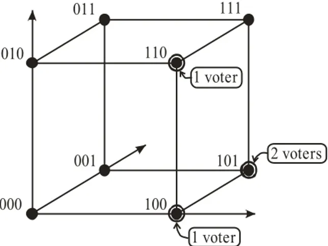
The Geometry Behind Paradoxes of Voting Power ... 193 S. Kaci, L. van der Torre
J. Lang
Vote and aggregation in combinatorial domains with structured preferences ... 257 D. Lozovanul, S. Pickl
Multilayered Decision Problems ... 273 Th. Marchant
A simple Bayes factor for testing measurement-theoretic axioms... 279 B. Monjardet
Condorcet domains and distributive lattices... 285 M. Öztürk, A. Tsoukiàs
New results on interval comparison ... 303 E. Pacuit, R. Parikh
Knowledge Considerations in Strategic Voting ... 323
M. S. Pini, F. Rossi, K. Venable, T. Walsh
Preference aggregation and elicitation : tractability in the presence of incomple- teness and incomparability ... 335
bipolar-valued outranking digraph
Raymond Bisdorff *
Abstract
In this paper we would like to thoroughly cover the problem of computing all kernels, i.e. minimal outranking and/or outranked independent choices in a bipolar-valued outranking digraph. First we introduce in detail the concept of bipolar-bipolar-valued characterisation of outranking digraphs, choices and kernels. In a second section we present and discuss several algorithms for enumerating the kernels in a crisp digraph. A third section will be concerned with extending these algorithms to bipolar-valued outranking digraphs.
Key words : Graph Theory, Maximum Independent Sets, Enumerating Kernels,
Out-ranking Digraphs
∗Applied Mathematics Unit, University of Luxembourg, 162a, avenue de la Fa¨ıencerie, L-1511 Luxem-borg,http://sma.uni.lu/bisdorff
Contents
1 Kernels in bipolar valued directed graphs 3
1.1 Bipolar-valued credibility calculus . . . 3
1.2 The bipolar-valued outranking digraph . . . 5
1.3 On choices and kernels in bipolar-valued outranking digraphs . . . 9
1.4 Bipolar-valued characterisation of choice classes . . . 14
2 Enumerating crisp kernels 18 2.1 Enumerating minimal and maximal qualified choices . . . 18
2.2 Complexity and performance . . . 22
2.3 Qualified choices graph traversal algorithms for kernel enumeration . . . 23
2.3.1 Reducing outranking choices . . . 24
2.3.2 Extending independent choices . . . 25
2.3.3 Outranking and outranked kernels in the same run . . . 26
2.4 Complexity and computational performance . . . 27
3 Algebraic approach 29 3.1 The kernel characteristic equations . . . 29
3.2 Solving the kernel characteristic equation system . . . 32
3.2.1 Smart enumeration with a finite domain solver . . . 32
3.2.2 Fixpoint based solving approaches . . . 32
Introduction
Minimal independent and outranking or outranked choices, i.e. kernels, in valued out-ranking digraphs are an essential formal tool for solving best unique choice problems in the context of our multicriteria decision aid methodology [10]. It appears, following recent formal results [8], that computing these kernels may rely on the enumeration of all kernels observed in the associated crisp median cut outranking digraph. Knowing these crisp kernels allows one to compute the associated bipolar-valued kernel via the fixpoints of the kernel bipolar-valued characteristic equation systems. In this article we shall therefore, first, present the bipolar-valued concepts of outranking digraphs and in-dependent outranking and outranked choices, each associated with their corresponding median cut crisp concept. In a second section, we shall then discuss general algorithms for enumerating crisp outranking and/or outranked choices in a bipolar-valued digraph. A third section will be devoted to extending these algorithms in order to compute the corresponding bipolar-valued choices.
1
Kernels in bipolar valued directed graphs
In this first section we introduce the fundamental concepts and notations about bipolar-valued outranking graphs and kernels.
1.1
Bipolar-valued credibility calculus
Letξ be a propositional statement like – decision alternative a is a best choice – or –
decision alternative a is at least as good as decision alternative b. In a decision process,
a decision maker may either accept or reject these statements following his degree of confidence in their truth [6].
Definition 1 (Bipolar-valued credibility calculus)
The degree of confidence in the truth – the credibility – of a statement may be represented with the help of a rational credibility scaleL = [−1, 1] supporting the following truth-denotation semantics:
1. Letr ∈ L denote the credibility of a statement ξ. If r = +1 (resp. r = −1) then it is assumed thatξ is certainly true (resp. false). If 0 < r < +1 (resp. −1 < r < 0) then it is assumed thatξ is more true than false (resp. more false than true). If r = 0 thenξ is logically undetermined, i.e. ξ could be either true or false;
2. Letξ and ψ be two propositional statements to which are associated credibilities r ands ∈ L. If r > s > 0 (resp. r < s < 0) then it is assumed that the truth (resp. falsity) ofξ is more credible than that of ψ;
3. Letξ and ψ be two propositional statements to which are associated credibilities r ands ∈ L. The truthfulness of the disjunction ξ ∨ ψ (resp. the conjunction ξ ∧ ψ) of these statements corresponds to the maximum of their credibilities: max(r, s) (resp. the minimum of their credibilities:min(r, s)).
4. Ifr ∈ L denotes the degree of confidence in the truth of a propositional statement ξ, then −r ∈ L denotes the degree of confidence in its untruth, i.e. the credibility of the logical negation ofξ (¬ξ).
The credibility degree associated with the truth of a propositional statementξ and defined in a credibility domainL verifying properties (1) to (4), will be called a bipolar-valued characterisation ofξ.
A consequence of Definition 1 is that the graduation of confidence degrees concerns nec-essarily at the same time the affirmation as well as the negation of a propositional state-ment [30]. Starting from+1 (certainly true) and −1 (certainly false) one can approach the central undetermined degree of credibility0 by a gradual weakening of the degrees of confidence. This central point inL is a so-called negational fixpoint [6; 7].
Definition 2
The degree of logical determination ( determinateness for short)D(ξ) of a propositional statementξ is given by the absolute value of its bipolar-valued characterisation: D(ξ) = |r|.
For both a certainly true and a certainly false statement, the determinateness will be1. On the contrary, for an undetermined statement, this determinateness will be0.
This clearly establishes the central degree0 as an important neutral value in the bipolar credibility calculus. Propositions characterised with this degree0 may be seen, either as
suspended, or as missing statements[7]. This situation corresponds to what we call a suspension of judgment. It is a temporary delay in characterising the actual truth or falsity
of a propositional statement, which may become eventually determined, either as a more true than false, or as a more false than true statement, in a later stage of the decision aiding process.
1.2
The bipolar-valued outranking digraph
Our starting point is a decision aiding problem on a finite setX = {x, y, z, . . .} of deci-sion objects (or alternatives), evaluated on a finite, coherent familyF = {1, . . . , p} of p criteria. To each criterionj of F is associated its significance represented by a rational numberwjfrom the open interval]0, 1[ such thatPpj=1wj= 1. Besides, to each criterion j is connected a rational (normalised) preference scale in [0, 1] which allows to compare the performances of the decision objects on the corresponding preference dimension.
Letgj(x) and gj(y) be the performances of two alternatives x and y of X on criterion j. The difference of the performances gj(x) − gj(y) is written ∆j(x, y). Each preference scale for each criterionj supports a rational indifference threshold hj ∈ [0, 1[, a weak preference thresholdqj ∈ [hj, 1[, a weak veto threshold wvj ∈ [qj, 1] ∪ {2} and a strong veto thresholdvj ∈ [wvj, 1] ∪ {2}, where the complete absence of veto is modelled via the value2.
Classically, an outranking situationx S y between two decision alternatives x and y ofX is assumed to hold if there is a sufficient majority of criteria which support an “at
least as good” preferential statement and there is no criterion which raises a veto against
it [24]. As we are going to show, this definition leads quite naturally to a bipolar-valued characterisation of binary outranking statements.
Indeed, in order to characterise a local “at least as good” situation between alterna-tivesx and y of X on each criterion j ∈ F , we use the following criterion-function: Cj : X × X → {−1, 0, 1} such that: Cj(x, y) = 1 if ∆j(x, y) > −hj; −1 if ∆j(x, y) ≤ −qj; 0 otherwise.
Following the truth-denotation semantics of the bipolar-valued characterisation, deter-minateness0 is assigned to Cj(x, y) in case it cannot be determined whether alternative x is at least as good as alternativey or not (see Subsection 1.1).
Similarly, the local veto situation on each criterionj ∈ F is characterised via a crite-rion based veto-function:Vj : X × X → {−1, 0, 1} where:
Vj(x, y) = 1 if ∆j(x, y) ≤ −vj; −1 if ∆j(x, y) > −wvj; 0 otherwise.
According again to the semantics of the bipolar-valued characterisation, the veto function Vjrenders a logically undetermined response when the loss in performances between two alternatives lies in between the weak and the strong veto thresholdswvjandvj.
The global outranking index eS, defined between all pairs of alternatives x, y ∈ X, conjunctively combines a global concordance index – aggregating all local “at least as
good” statements –, and the absence of a veto observed on an individual criterion.
eS(x, y) = min{ ˜C(x, y), −V1(x, y), . . . , −Vp(x, y)}, (1) where the global concordance index ˜C(x, y) is defined as follows:
˜
C(x, y) =X j∈F ¡
wj· Cj(x, y)¢ ∀x, y ∈ X. (2)
The min operator in Formula (1) translates the conjunction between the global concor-dance index ˜C(x, y) and the negated criterion based veto indexes −Vj(x, y) (∀j ∈ F ). in the case of absence of veto, the resulting outranking index eS equals the global con-cordance index ˜C. Following Formulas (1) and (2), eS is a function from X × X to L representing the degree of confidence in the truth of the outranking situation observed between each pair of alternatives. eS will be called the bipolar-valued characterisation of the outranking situationS, or for short a bipolar-valued outranking relation.
The maximum possible value of the valuation eS(x, y) = +1 is reached in the case of unanimous concordance, whereas the minimum value eS(x, y) = −1 is obtained either in the case of unanimous discordance, or if we observe a veto situation on some criterion. The median situation0 represents a case of indeterminateness: either there are neither enough arguments in favour nor against a given outranking statement or, a potentially sufficient majority in favour of the outranking is outbalanced by an undetermined, i.e. potential veto situation.
We can easily recover the truth-denotation semantics from the previous Subsection (1.1). For any two alternativesx and y of X,
– eS(x, y) = +1 signifies that the statement “x S y” is certainly true;
– eS(x, y) > 0 signifies that statement “x S y” is more true than false. A sufficient majority of criteria warrants the truth of the outranking;
– eS(x, y) = 0 signifies that statement “x S y” is logically undetermined, i.e. could be
either true or false;
– eS(x, y) < 0 signifies that assertion “x S y” is more false than true. There is only a minority of the criteria which warrants the truth of the outranking. This is equivalent to saying that a sufficient majority of criteria warrants the truth of the negation of the outranking;
Definition 3
The setX associated to a bipolar-valued characterisation eS of the outranking relation S ∈ X × X is called a bipolar-valued outranking digraph, denoted eG(X, eS).
From the truth-denotation semantics of a bipolar-valued characterisation it results that we can recover the crisp outrankingS characterised via eS as the set of pairs (x, y) such that eS(x, y) > 0. We write G(X, S) the corresponding so-called strict 0-cut crisp outranking
digraph associated to eG(X, eS). Example 1
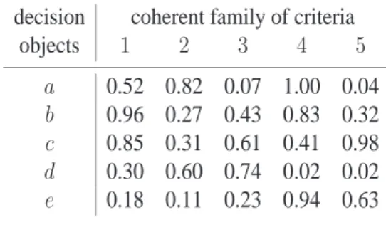
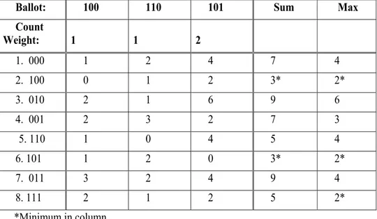
In order to illustrate the concept of bipolar-valued outranking graph, we consider a set X1 = {a, b, c, d, e} of five decision alternatives evaluated on a coherent family F1 = {1, . . . , 5} of five criteria of equal significance. On each criterion we observe a rational preference scale from0 to 1 with an indifference threshold of 0.1, a preference thresh-old of0.2, a weak veto threshold of 0.6, and a veto threshold of 0.8. Table 1 shows a randomly generated performance table [11]. Based on the performances of the five
al-decision coherent family of criteria
objects 1 2 3 4 5 a 0.52 0.82 0.07 1.00 0.04 b 0.96 0.27 0.43 0.83 0.32 c 0.85 0.31 0.61 0.41 0.98 d 0.30 0.60 0.74 0.02 0.02 e 0.18 0.11 0.23 0.94 0.63 Table 1: Example 1: Random performance table
ternatives on each criterion, we compute the bipolar-valued outranking relation eS1shown in table 2. The strict 0-cut crisp digraphG1(X1, S1) associated to the bipolar-valued
eS1 a b c d e a 1.0 -0.2 -1.0 0.6 0.4 b 0.4 1.0 0.2 0.2 0.4 c 0.2 0.4 1.0 0.4 0.6 d -1.0 -1.0 -1.0 1.0 -1.0 e 0.2 0.2 -0.4 0.0 1.0
? e b
d a
c
Figure 1: Example 1: Associated strict 0-cut digraph and undetermined arc
outranking digraph eG1(X1, eS1) is shown in figure 1. We have also represented the unde-termined arc from alternativee to d which represents an undetermined outranking. This situation is not expressible in a standard Boolean-valued characterisation of the outrank-ing. Consequently, the (‘positive’) negation of the general eS relation is not identical with the complement ofS in X × X.
Let us finish this subsection by introducing some concepts which will be used in the sequel.
A bipolar-valued digraph eG(X, eS) such that eS(x, y) > 0 for all x, y in X will be called
determined. If eS(x, y) = 0 for some pairs (x, y), we call eG partly determined.
The ordern of the digraph eG(X, eS) is given by the cardinality of X, whereas the size m of eG is given by the cardinality of S. As X is a finite set of n alternatives, the size m of the digraph eG is also finite. The arc density δ of eG is given by the ratio of the size over the maximal number of possible arcs in the graph:
δ = m
n × n (3)
In example 1, the order of eG1equals 5 and its size 13, such that its arc density is 52%. A digraph eG(X, eS) is said to be empty if the size of G(X, S) equals 0, i.e. S = ∅. On the opposite, a digraph eG(X, eS) is said to be complete if G(X, S) = Kn, i.e.S = X × X. A digraph eG(X, eS) of order n is said to be connected if the symmetric and transitive closure ofG(X, S) equals Kn.
A path of orderm ≤ n in eG(X, eS) is a sequence (xi)m
i=1 of alternatives ofX such that eS(xi, xi+1) > 0, ∀i ∈ {1, . . . , m − 1}. A circuit of order m ≤ n is a path of order m such that eS(xm, x1) ≥ 0. An cordless circuit (xi)m
i=1is a circuit of orderm such that eS(xi, xi+1) > 0, ∀i ∈ {1, . . . , m − 1}, eS(xm, x1) > 0 and eS(xi, xj) < 0 otherwise. A path or circuit will be called weak when it contains one or more zero-valued arcs.
Following a result by Bouyssou [12; 13] it appears that, apart from certainly being reflexive, the bipolar-valued outranking digraphs do not necessarily possess any special
relational properties such as transitivity or complete comparability. Indeed, with a suf-ficient number of criteria, it is always possible to define an ad hoc performance table such that the associated crisp 0-cut outranking digraph renders any given reflexive binary relation. This rather positive result from a methodological point of view – the outrank-ing based methodology is universal – bears however a negative algorithmic consequence. Enumerating all kernels in a bipolar-valued outranking digraph becomes a non trivial al-gorithmic problem in case of non-transitive and partial outrankings, as we will show in the next section.
Before tackling this main topic of this work, let us, first, finish this section with intro-ducing bipolar-valued choices and kernels.
1.3
On choices and kernels in bipolar-valued outranking digraphs
A choice in a given bipolar-valued outranking digraph is a non-empty subset of decision objects.
Definition 4
1. A choiceY in eG(X, eS) is said to be outranking (resp. outranked) if and only if x 6∈ Y ⇒ ∃y ∈ Y : eS(y, x) > 0 (resp. eS(x, y) > 0);
2. Y is said to be independent (resp. weakly independent) if and only if for all x 6= y inY we have eS(x, y) < 0 (resp. eS(x, y) 6 0;
3. An outranking (resp. outranked) and independent choice will be called an outrank-ing(resp. outranked) kernel;
4. An outranking (resp. outranked) and weakly independent choice will be called a weakoutranking (resp. outranked) kernel.
Example 2 (Example 1 continued)
In the strict0-cut crisp digraph G1(see Figure 1) we can observe two outranking kernels, namely the single choices {b} and {c}. The digraph also contains a weak outranked kernel, namely the pair{d, e}. Indeed, alternatives d and e are only weakly independent one from the other.
Let us finish this first section with presenting some interesting properties that ker-nels in their quality as independent outranking, resp. outranked, choices do possess. To illustrate this part, we use the following example.
Example 3 (B. Roy (2005), private communication)
Let eG2(X, ˜S1) be the bipolar-valued digraph where: X2 = {a, b, c, d, e} and ˜S2is given as follows:
˜ S2 a b c d e a - 0.6 -1.0 -0.7 -0.9 b -0.8 - 0.9 1.0 0.0 c -1.0 -1.0 - 0.6 0.9 d 0.8 -0.8 -1.0 - -0.7 e -1.0 -0.9 -0.7 -0.8 -? b a d c e
The associated strict 0-cut digraph
b a
d
c e
{a, b, d, e} is an outranking choice.
b a
d
c e
{b, d, e} is an outranked choice.
In example (3), we may notice that the outranking choice{a, b, d, e} in eG2(see exam-ple 3) may be reduced without loosing the property of being outranking. The outranked choice in the same example (3) may not however be reduced without loosing its out-rankedness property. Minimal or maximal cardinality of choices with respect to a given qualification is formally captured in the following definition.
Definition 5 (Qualified choices of minimal or maximal cardinality)
A choiceY in eG, verifying a property P , is minimal with this property whenever, ∀Y′∈ e
G which verify the same property P , we have Y′ 6⊆ Y . Similarly, a choice Y in eG, verifying a propertyP , is maximal with this property whenever, ∀Y′ ∈ eG which verify propertyP , we have Y′6⊇ Y .
Example 4 (Minimal qualified choices in eG2)
b a
d
c e
{a, c} is a minimal outranking choice.
b a
d
c e
Comparing the outranking choice{a, b, d, e} in example (3) with the minimal out-ranking choice{a, c} in example (4) we may notice that minimality of outrankingness, resp. outrankedness, is related to the neighbourhoods of the nodes of the digraph.
We denoteN+(x) = {y ∈ X / eS(x, y) > 0} the open outranked neighbourhood of a nodex ∈ X. We denote N+[x] = N+(x) ∪ {x} the closed outranked neighbourhood of x. We denote N−(x) = {y ∈ X / eS(y, x) > 0} the open outranking neighbourhood of a nodex. We denote N−[x] = N−(x) ∪ {x} the closed outranking neighbourhood of x.
The neighbourhood concept may easily be extended to a choice. The closed and open
outranked neighbourhood of a choiceY in eG are given by the union of the respective neighbourhoods of the members of the choice:
N+[Y ] = [ x∈Y
N+[x], N+(Y ) = [ x∈Y
N+(x). (4)
The closed and open outranking neighbourhood of a choiceY in eG are similarly given by the union of the respective elementary outranking neighbourhoods:
N−[Y ] = [ x∈Y
N−[x], N−(Y ) = [ x∈Y
N−(x). (5)
Definition 6 (Private neighbourhood)
The (closed) private outranked neighbourhoodNY+[x] of a node x in a choice Y contain-ingx is defined as follows: NY+[x] = N+[x] − N+[Y − {x}]. Similarly, the (closed) private outranking neighbourhoodNY−[x] of a node x in a choice Y is defined as follows: NY−[x] = N−[x] − N−[Y − {x}]. In case of a single choice, both the outranked and the outranking neighbourhood are considered to be private by convention.
In the outranking choiceY = {a, b, d, e} of example (3), we may notice that action a for instance has no private outranked neighbourhood. IndeedNY+[a] = N+[a] − N+[Y − {a}] where N+[a] = {a, b} and N+[Y − {a}] = X. Action b however has action c as private outranked neighbourhood. The concept of private neighbourhoods leads us naturally to the notion of irredundant choices.
Definition 7 (±-irredundant choice)
An outranking choiceY in eG is called +irredundant if and only if all its members have a non empty private outranked neighbourhood, i.e. ∀x ∈ Y : N+
Y[x] 6= ∅. Similarly, an outranked choiceY in eG is called -irredundant if and only if all its members have a private outranking neighbourhood, i.e.∀x ∈ Y : N−
Y[x] 6= ∅.
In example (4), the outranking choice {a, c} is +irredundant as N{a,c}+ [a] = {a, b} and N{a,c}+ [c] = {c, d, e}. Similarly the outranked choice {b, d, e} is -irredundant as N{b,d,e}− [b] = {a, b}, N{b,d,e}− [d] = {c} and N{b,d,e}− [e] = {e}.
Minimality of outrankingness (resp. outrankedness) and maximality of±-irredundancy are evidently linked.
Proposition 1
(i) An outranking (resp. outranked) choice Y in eG is minimal outranking (resp. out-ranked) if and only if it is outranking (resp. outout-ranked) and +irredundant (resp. -irredundant) (Cockayne, Hedetniemi, Miller 1978).
(ii) Every minimal outranking (resp. outranked) choiceY in eG is maximal +irredundant (resp. -irredundant) (Bollob´as, Cockayne, 1979).
Proof: Property (i) following easily from property (2), we demonstrate only the latter one.
[⇒] Let us suppose that Y is minimal outranking but not maximal +irredundant. This implies that there exists a nodex ∈ X − Y such that Y ∪ {x} is +irredundant, i.e. N+(Y ) is a proper subset ofN+(Y ∪{x}). This contradicts however the fact that Y is outranking. [⇐] The other way round, let us suppose that Y is maximal +irredundant but not minimal outranking. This implies that there must exist an y ∈ Y such that Y − {y} still remains outranking, i.e. thisy cannot have a private outranked neighbourhood with respect toY . This contradicts however the hypothesis that Y is +irredundant.
A similar reasoning is valid for outranked and -irredundant choices. 2
Similarly, maximal independence and minimal outrankingness or outrankedness are tightly related.
Proposition 2 (Berge, 1958)
Let eG(X, eS) be a determined bipolar-valued digraph. (i) Every kernel is a minimal out-ranking (resp. outranked) choice. (ii) Every minimal outout-ranking (resp. outranked) and independent choice is maximal independent.
Proof: (1) Let us suppose that an outranking kernelY is indeed not a minimal outrank-ing (respectively outranked) choice. This implies that there exists an outrankoutrank-ing (respec-tively outranked) choiceY′⊂ Y such that Y′is still outranking (respectively outranked). This implies that ∀y ∈ Y − Y′ there must exist somey′ ∈ Y′such that (y, y′) ∈ S (respectively(y′, y) ∈ S. This is contradictory with the fact that Y is independent. (2) Let us suppose that an outranking kernelY is indeed not a maximal independent choice. This implies that there must exist aY′⊃ Y such that Y′is still independent. ButY is by hypothesis an outranking (respectively outranked) choice, i.e. ∀y′ ∈ Y′− Y there must exist somey ∈ Y such that (y, y′) ∈ S (respectively (y′, y) ∈ S. Hence there appears again a contradiction. 2
Not all minimal outranking (resp. outranked) choices are independent, i.e. kernels. In digraph eG2of example 3, for instance, we observe the following four minimal outranking choices, of which only choice{a, c} is independent and therefore an outranking kernel.
b a
d
c e
minimal outranking choice,
b a
d
c e
minimal outranking choice.
b a d c e outranking kernel, b a d c e
minimal outranking choice.
Kernels and minimal choices however coincide in determined and transitive digraphs. Proposition 3
Let eG(X, eS) be a transitive and determined digraph, i.e. the associated crisp graph G(X, S) supports a transitive outranking relationS. A choice Y in eG is an outranking (resp. out-ranked) kernel if and only ifY verifies one of the following equivalent conditions:
1. Y is minimal outranking (resp. outranked); 2. Y is outranking (resp. outranked) and independent; 3. Y is outranking (resp. outranked) and +(-)irredundant; 4. Y is maximal +(-)irredundant.
Proof: (1)⇔ (3) ⇔ (4) are covered by proposition 1, and (2) ⇒ (1) is covered by proposition 2. We only need to prove that (1)⇒ (2).
Let us therefore suppose that a minimal outranking (respectively outranked) choiceY is indeed not independent. As eG is determined, this implies that there exists some proper subsetY′⊂ Y such that for y ∈ Y − Y′andy′∈ Y′we observe(y, y′) ∈ S (respectively (y′, y) ∈ S. As Y is a minimal outranking (respectively outranked) choice, each action inY must have a private outranked (resp. outranking) neighbourhood and in particular all actions in Y′. By transitivity ofS, the private neighbourhoods N+
of an actiony′ ∈ Y′are transferred toy ∈ Y − Y′. AndY − Y′remains therefore an outranking (resp. outranked) choice. This is however contradictory with the hypothesis thatY is minimal with this quality. 2
It is worthwhile noticing that proposition (3) only applies to determined digraphs. In case we observe a partially determined graph, it may happen that a minimal outranking (resp. absorbent) choice is only weakly independent, and vice-versa, it may indeed happen that a maximal independent choice is neither outranking nor outranked. All depends upon the particular presence of undetermined relations.
We have not the space in this paper to present all existence results for kernels in a digraph (see for instance [19]). Relevant properties for our purpose are summarized below, where we generally suppose that the bipolar-valued digraph is determined. Proposition 4 (Existence of qualified choices)
1. Every digraph supports minimal outranking (resp. outranked), as well as maximal independent and/or +irredundant (resp. -irredundant) choices.
2. A transitive digraph always supports an outranking (resp. outranked) kernel and all its kernels are of same cardinality (K¨onig, 1950 [22]).
3. A symmetric digraph always supports a conjointly outranking and outranked kernel (Berge, 1958 [1]).
4. An acyclic digraph always supports a unique outranking (resp. outranked) kernel (Von Neumann, 1944 [29]).
5. If a digraph does not contain any cordless circuit of odd length, it supports an out-ranking (resp. outranked) kernel (Richardson, 1953 [23]).
1.4
Bipolar-valued characterisation of choice classes
In the previous sections we have worked with different kinds of choices, namely out-ranking, outranked, independent, ±-irredundant ones. Similarly to the bipolar-valued characterisation of the digraph, we may now define a bipolar-valued characterisation of these kinds or classes on the power setP(X) of all possible choices we may define in eG. As these classes are all defined with logical conditions applied on bipolar-valued bi-nary outranking statements, we first need to extend the bipolar-valued credibility calculus to well formed logical expressions.
Definition 8 (Well formed logical expressions)
LetG denote a set of ground atomic logical statements. We define inductively the set E of well formed logical expressions in the following way:
1. ∀p ∈ G we have p ∈ E;
2. ∀x, y ∈ E we have (x ∨ y) ∈ E, (x ∧ y) ∈ E, and ¬x ∈ E 3. allp ∈ E result of finite construction.
In order to avoid any problem with precedence of operators, we shall always use brackets to delimit the scope of the logical operatorsmax, min and ¬ in an expression. Here our ground atomic logical expressions are the binary outranking assertionsx S y of the given digraph eG(X, eS). Our well formed logical expressions concern formulas involving these binary outranking assertions.
As the atomic outranking assertions are evaluated in the given digraph eG(X, eS), fol-lowing the truth-denotation semantics of Definition 1, we are now able to evaluate any well formed logical expression involving these evaluations eS(x, y). We start by defining the degree of±-irredundancy of a choice in eG.
Definition 9 (Bipolar-valued±-irredundance of choices)
Let eG(X, eS) be a bipolar-valued digraph. The credibility of (outranking) +irredundancy of actionx with respect to choice Y in eG is given by:
∆+irr
Y (x) = (
+1.0 when Y = {x},
max(z,y)∈X×Y −{x}min¡ eS(x,z),−eS(y,z) ¢ otherwise. (6) Similarly, the credibility of (outranked)−irredundancy of action x with respect to choice Y in eG is given by:
∆-irr
Y (x) = (
+1.0 when Y = {x},
max(z,y)∈X×Y −{x}min¡ eS(z,x),−eS(z,y) ¢ otherwise. (7) The credibility of +irredundancy of choiceY in eG is given by:
∆+irr(Y ) = min
x∈Y ∆
+irr
Y (x) (8)
The credibility of -irredundancy of choiceY in eG is given by: ∆-irr(Y ) = min
x∈Y ∆
-irr
Y (x) (9)
Proposition 5
Y in eG is a +irredundant outranking (resp. -irredundant) choice if and only if ∆+irr(Y ) > 0
Proof: (⇒) Suppose ∆+irr(Y ) < 0. Then ∃x ∈ Y such that ∆+irr
Y (x) < 0. This implies thatY ⊂ X and ∀(z, y) ∈ X × Y − {x} we have min¡ eS(x,z),−eS(y,z)¢ < 0. In other terms:∀z ∈ N+[x] : ∃y ∈ Y − {x} such that z ∈ N+[y]. Hence x is redundant and Y cannot be +irredundant.
(⇐) Let us suppose the other way round that x in choice Y is redundant. This implies thatNY + [x] = ∅. In other terms: N[x] − N+[Y − {x}] = ∅. This is exactly the case when for allz ∈ X such that eS(x, z) > 0, we find a y ∈ Y − {x} such that eS(y, z) > 0. In this casemax(z,y)∈X×Y −{x}(eS(z, x), −eS(z, y)) < 0 and ∆+irr
Y (x) < 0. A same development applies for the outranked case. 2
Definition 10 (Bipolar-valued qualification of choices)
Let eG(X, eS) be a bipolar-valued digraph. The credibility of outrankingness of a choice Y in eG is given by:
∆dom(Y ) =
(
+1.0 when Y = X,
minx6∈Ymaxy∈Y¡eS(y,x)¢ otherwise. (10)
The credibility of outrankedness of a choiceY in eG is given by: ∆abs(Y ) =
(
+1.0 when Y = X,
minx6∈Y maxy∈Y¡eS(x,y)¢ otherwise. (11)
The credibility of independence of a choiceY in eG is given : ∆ind(Y ) =
(
+1.0 if Y = {x},
miny6=xy∈Yminx∈Y¡− eS(x, y)¢ otherwise. (12) Proposition 6
Let eG(X, eS) be an bipolar-valued outranking graph.
1. Y in eG is an independent (resp. weakly independent) choice if and only if∆ind(Y ) >
0 (resp. ∆ind(Y ) > 0).
2. Y in eG is an outranking (resp. outranked) choice if and only if∆dom(Y ) > 0 (resp.
∆abs(Y ) > 0).
Proof: Property (1) follows immediately from definition (2) which states that a choice Y is indeed independent (weakly independent) if and only if eS(x, y) > 0 (eS(x, y) 6 0) for allx, y ∈ Y .
Property (2), similarly, follows immediately from definition (1), as a choiceY is out-ranking (resp. outranked) if and only if∀x ∈ Y : ∃y ∈ Y such that eS(y, x) > 0 (resp. eS(y, x) > 0). 2
Corollary 1
Let eG(X, eS) be an bipolar-valued outranking graph and G(X, S) its associated strict 0-cut crisp digraph. The minimal outranking (resp. outranked) choices of eG correspond to the minimal outranking (resp. outranked) choices ofG.
Proof: Y in eG is a minimal outranking (resp. outranked) choice if and only if ∆+irr(Y ) >
0 and ∆dom(Y ) > 0 (resp. ∆-irr(Y ) > 0 and ∆abs(Y ) > 0). 2
This important result from an operational point of view allows to determine the bipolar-valued minimal outranking (resp. outranked) choices in a bipolar-bipolar-valued digraph eG as follows:
1. Compute the minimal outranking (resp. outranked) crisp choices in the associated strict 0-cut digraphG, and
2. Compute the credibility of their qualification.
Corollary 2 (Kitainik 1993)
The set of outranking (resp. outranked) kernels of eG is a subset of the set of outranking (resp. outranked) kernels of the associated strict 0-cut crisp digraphG.
Proof: Let eG(X, eS) be a bipolar-valued outranking graph. Y in eG is an outranking (resp. outranked) kernel if and only if∆ind(Y ) > 0 and ∆dom(Y ) > 0 (resp. ∆abs(Y ) > 0). 2
It is worthwhile noting, that the actual set of kernels in the associated strict 0-cut digraph G may be larger than than that of the original bipolar-valued digraph eG. It may con-tain, the case given, some outranking or outranked choices, that are indeed only weakly independent. These weak kernels correspond to partly determined choices.
Kitainik’s result allows us to determine all possible outranking or outranked (weak) kernels in a bipolar-valued digraph eG as follows:
1. We extract all crisp kernels and weak kernels from the associated strict 0-cut crisp graphG and,
2. for each such crisp kernel or weak kernel inG, we compute in eG its bipolar-valued credibility.
Enumerating in a bipolar-valued digraph all outranking and outranked crisp kernels will actually be the purpose of the next section.
2
Enumerating crisp kernels
Enumerating kernels necessarily relies on general techniques for enumerating qualified choices, like minimal outranking or maximal independent ones. We start this section with the presentation of a general framework for enumerating such minimal or maximal qualified choices. After the discussion of their complexity and performance, we present and discuss specific algorithms for enumerating outranking as well as outranked crisp kernels.
2.1
Enumerating minimal and maximal qualified choices
Definition 11 (Hereditary properties)
A propertyP of choices is said to be hereditary0 if whenever a choiceY has property
P , so does every proper subchoice Y′ ⊂ Y . A property P of choices is said to be superhereditaryif whenever a choiceY has property P , so does every proper superchoice Y′⊃ Y .
Proposition 7
Being outranking or outranked are superhereditary properties of choices in eG. Similarly, independence as well as±-irredundancy are hereditary properties of choices in eG. Proof: Hereditary follows immediately from the definition of an independent, an +ir-redundant, and an -irredundant choice. Superhereditary follows again readily from the definition being outranking or outranked. 2
Inheritance of being outranking makes it possible to implement the search for minimal outranking choices as a path algorithm in the outranking choices graph associated with
e G.
Definition 12 (P -choices graphs)
Let eG(X, eS) be an outranking graph. Let P(X) represent the powerset of choices in eG with propertyP . The couple H(P(X), P ) is called the P choices-graph associated with
e
G. Two choices are linked in H(P(X), P ) if they have some common action.
0The ideas and results concerning hereditary and superhereditary properties of choices are taken from [20, see Chapter 3].
Proposition 8
1. The outranking and outranked choices graphs associated with eG contain the greedy choiceX and are each one strongly connected,
2. The±-irredundant and independent choices graphs associated with eG are composed of a set of strongly connected components such that each singleton choice belongs to exactly one component.
Proof: Ad 1. As outrankingness and outrankedness are superhereditary properties, there necessarily exists a path from every possible minimal outranking (resp. outranked) choice toX, the largest outranking (resp. outranked choice) and vice versa.
Ad 2. Both irredundancies as well as the independence property being hereditary, there necessarily exists a path in the corresponding choices-graphs from a maximal ±-irredundant (resp. independent) choice to each of its single choice members and vice versa. 2
Following proposition 8, enumerating all minimal outranking or outranked choices may be implemented as a graph traversal algorithm in the corresponding choices graphs, where we try to explore all paths from the largest outranking (resp. outranked) choice – the greedy choiceX – to the first subchoices which are ±-irredundant.
Algorithm 1 (Enumerating minimal outranking choices) globalHist
Hist ← ∅ # initialise the history Y0 ← X # start with the greedy choice K0+ ← ∅ # initialise the result
K+ ← MinimalOutrankingChoices(Y0, K+ 0)
defMinimalOutrankingChoices(In: Yioutranking,Ki+; Out:Ki+1+ ) K+← ∅
IRRED ← True
for[x ∈ Yi: NYi+[x] = ∅]: # Retract in turn all redundant nodes IRRED ← False
Yi+1 ← Yi− {x} #Yi+1remains outranking ! ifYi+16∈ Hist:
K+ ← K+∪MinimalOutrankingChoices(Yi+1, K+): Hist ← Hist ∪ {Yi+1}
ifIRRED:
Ki+1+ + ← Ki+∪ Y #Y is +irredundant (and outranking) else:
Ki+1+ + ← Ki+∪ K+ returnKi+1+
Proof: The algorithm starts with the greedy choiceY = X which is always outranking and an empty set of minimal outranking choices.
The procedureMinimalOutrankingChoicescollects all minimal outranking choices that may be reached from the initial outranking choiceY .
The call invariants of procedureMinimalOutrankingChoicesare that the choice Yiis outranking andKi+is a set of minimal outranking choices collected so far.
IfYiis outranking, thenYi+1= Yi− {x} is constructed only if N+
Yi[x] = ∅, i.e. in case x is a +redundant action and Yi+1remains outranking. If no more +redundant actions may be found, the procedure stops the walk. AsY0 = X is outranking, the algorithm walks therefore only on paths of the outranking choices-graph.
Let us suppose that at calli, Ki+contains only minimal outranking choices. Two sit-uations may happen. Either the current choiceYiis irredundant or all redundant actions have been removed in turn. In the first case, we are in the presence of a maximal irre-dundant and dominating choice, i.e. a minimal outranking choice which is added to to the current setKi+. In the second case, all minimal outranking choices when reducing the current choice are first added up in a local resultK+ to be at the end added up toK+
i . This way,Ki+1+ can only contain minimal outranking choices. As we start with an empty initial collectionK0+, it is verified that in the endK+, if not empty, may only contain minimal outranking choices.
Finally, that we algorithm collects all existing minimal outranking choices in eG fol-lows from the fact that the outranking choices-graph is strongly connected and that there-fore, starting from the greedy choiceX, the algorithm walks necessarily through all out-ranking choices in eG. The global history we use keeps track of the visited outranking choices and avoids to explore several times the same outranking choice. 2
The same algorithm delivers the minimal outranked choices when replacing in the loop the private outranked neighbourhood with the corresponding private outranking neigh-bourhood. This way, we only walk on outranked choices and collect all minimal out-ranked choices instead.
Based again on proposition (8), we may design a similar graph traversal algorithm in the irredundant choices graph. This time, we try to explore all paths from the small-est +irredundant (resp. -irredundant) choices – the single choices – to all outranking or outranked choices we may find on our way.
Algorithm 2 (Enumerating maximal irredundant choices) globalHist
Hist ← ∅ # initialise the history K+ ← ∅ # initialise the result forx ∈ X:
K+ ← K+∪ MaxIrredOutrankingChoices(Y0, K+, Hist) defMaxIrredOutrankingChoices(In: Yi+irredundant,Ki+; Out:Ki+1+ ):
if(Yi− X) − N+(Yi) = ∅:
Ki+1+ ← Ki+∪ Yi #Yiis outranking else:
Ki+1+ ← Ki+ # initialise the result
for[x ∈ X − Yi: NYi+[x] 6= ∅]: # add all +irredundant actions Yi+1 ← Yi∪ {x}
ifYi+16∈ Hist:
Ki+1+ ← Ki+1+ ∪MaxIrredOutrankingChoices(Yi+1, Ki+1+ ): Hist ← Hist ∪ {Yi+1}
returnKi+1+
Proof: The algorithm starts with an empty history and an empty set of minimal out-ranking choices. The procedureMaxIrredOutrankingChoicesthen collects all minimal outranking choices that may be reached in turn from each initial single choice Y0= {x}, ∀x ∈ X
The call invariants of iterationi are that the current choice Yiis +irredundant andKi+ contains the minimal outranking choices collected so far.
IfYiis -irredundant, thenYi+1 = Yi∪ {x} is constructed only if NYi+[x] 6= ∅, i.e. in casex is a +irredundant action with respect to current choice Yi. Yi+1remains therefore +irredundant. As eachY0 is in turn +irredundant, the algorithm walks only on paths of the +irredundant choices graph.
Let us suppose that at iterationi, Ki+ is either empty or contains only minimal out-ranking choices. Two situations may happen. First, the current choiceYiis outranking and we have found a maximal irredundant, i.e. a minimal outranking choice, and we add it to the current setK+
i . In the second case, we gather all minimal outranking choices from the union of the current choiceYiwith all possible +irredundant actions, i.e. such thatN+
Yi[x] 6= ∅. This way, Ki+1+ can only contain minimal outranking choices or stay empty. As we start with an empty initial collectionK+
0, it is verified that in the endK+ may only contain minimal outranking choices.
Finally, that the algorithm collects all existing minimal outranking choices in eG fol-lows from the fact that the +irredundant choices-graph is composed of strongly connected components. Starting in turn from each single choice, the algorithm walks necessarily through all +irredundant choices existing inH(P(X), +irredundant). In order to avoid visiting the same +irredundant choices several times in turn from each member single choice, we keep a history of visited +irredundant choices, and only proceed recursively
with the next choiceYi+1in case it has not been visited already before. 2
The same algorithm delivers again the minimal outranked choices when replacing the outranked with the outranking neighbourhoods. This way, we only walk on -irredundant choices and collect all minimal outranked choices instead.
2.2
Complexity and performance
The problem of finding a minimal outranking or outranked choice of a certain cardinality k, is known to be NP-complete [18], so that there is little hope to find efficient algorithms for enumerating all minimal outranking or outranked choices in general digraphs of high orders.
Indeed, the complexity is directly linked to the size of theP -choices graphs. In case a bipolar-valued digraph is empty, only the greedy choice will actually be an outranking choice. The outranking choices graph reduces here to a single node and algorithm 1 will deliver immediately this unique possible solution. As every possible choice inP(X) will be irredundant, the corresponding±-irredundant choices-graph will be of order 2n− 1 (wheren is the order of eG) and of size (2n− 1)2− (2n− 1). Algorithm 2 therefore rapidly gets totally inefficient.
Similarly, in case eG is complete, i.e. G is a complete graph Kn, the irredundant choices-graph reduces ton isolated single choices. This time, algorithm 2 delivers imme-diately then solutions, whereas the corresponding outranking choices-graph is again of order2n− 1 and so of huge size (2n− 1)2− (2n− 1). Similarly, algorithm 1 this time is totally inefficient.
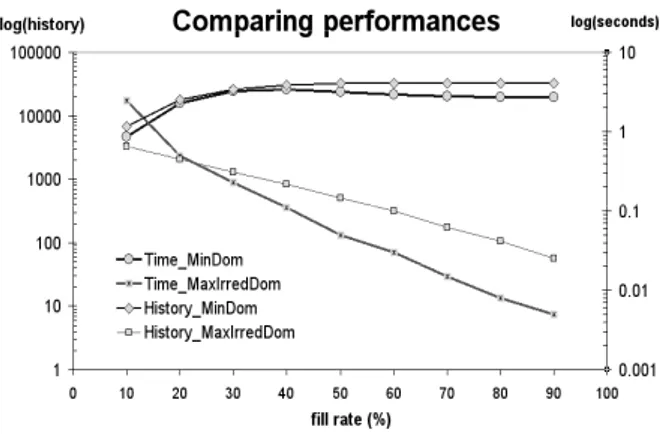
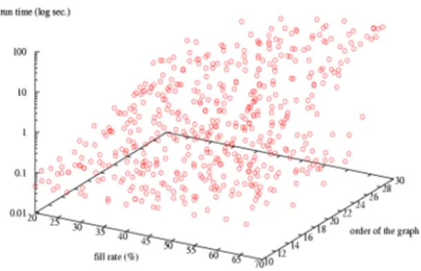
A stated before, we are mainly interested in dense digraphs where the second algo-rithm is more efficient in general, except for very low arc densities (see Figure 2.2). We have implemented both algorithms in the Python language (version 2.4) using the opti-mized inbuiltsetclass, which delivers constant time access to members of sets (indepen-dent of the cardinalities), and which offers optimized set operators like union, intersec-tion, and difference with linear time in the cardinality of the operands [11]. In figure (2.2) we have illustrated run time statistics for random digraphs of order 15 with arc densities varying from 10 to 90%.
It is obvious that theMaxIrredOutrankingChoicesalgorithm is doing much better except for arc densities below 15 %.
Let us now consider a special kind of outranking and outranked choices, namely those where the chosen actions are incomparable with respect to theS relation.
Figure 2: Run time statistics for randomly filled digraphs of order 15
2.3
Qualified choices graph traversal algorithms for kernel
enumer-ation
We have seen in the first section, that the independence property is computed from the false part of eS. In order to implement path algorithms in the corresponding independent-choices graph, we cannot, as usual rely on the false by failure principle, i.e. the comple-ment of the neighbourhoods, for representing independence. We need to introduce the logically positive concept of disconnects.
Definition 13 (Disconnects)
Let eG be an irreflexive digraph. We call disconnect of a node x, denoted D(x) = {y ∈ X : (eS(y, x) < 0) ∨ (eS(x, y) < 0)}, the set of nodes disconnected from x. We call disconnectof a choiceY , the intersection of disconnects of the members of Y :
D(Y ) = \ x∈Y
D(x). Proposition 9
A choiceY in eG is an outranking (respectively outranked) kernel if and only if: Y ⊆ D(Y ) (independent)
∀x 6∈ Y : N−(x) ∩ Y 6= ∅ (outranking) (resp.∀x 6∈ Y : N+(x) ∩ Y 6= ∅ (resp. outranked) )
Proof: It is readily seen that a choiceY is indeed independent if and only if the dis-connects of the choice members contain the otherwise chosen actions. Similarly, a choice
Y is outranking (resp. outranked) if and only if all not members of the choice are in the respective choice neighbourhood. 2
2.3.1 Reducing outranking choices
The previous result allows us to implement an outranking-choices graph traversal algo-rithm for enumerating all outranking kernels in a bipolar-valued outranking digraph. Algorithm 3 (Enumerating outranking kernels: variant 1)
Y0← X # start with the greedy choice K+←OutrankingKernels-1(Y0)
defOutrankingKernels-1(In: Y outranking; Out: K+) ifY ⊆ D(Y ):
K+← Y # Y is independent else:
K+← ∅ for[x ∈ Y : N+
Y[x] = ∅]: # Retract in turn all +-redundant nodes Y1 ← Y − {x} # Y 1 remains outranking !
K+ ← K+∪OutrankingKernels-1(Y1) returnK+
Proof: Similar in its design to algorithm 1, this algorithm starts again with the greedy choice Y = X which is always outranking by convention and an empty set of mini-mal outranking kernels. The procedureOutrankingKernelscollects all independent outranking choices that may be reached from this initial outranking choiceY .
The call invariants of iterationi are that the choice Yiis outranking andKi+is a set of outranking kernels collected so far.
IfYiis outranking, thenYi+1= Yi−{x} is constructed only if N+
Yi[x] = ∅, i.e. when x is a +irredundant action, so thatYi+1remains outranking. If no more +irredundant actions may be found, the procedure stops the walk. AsY0= X is outranking, the algorithm only walks on paths of the outranking choices-graph.
Let us suppose that at iterationi, Ki+contains only outranking kernels. Two situations may happen. Either the current choiceYiis independent or all redundant actions have been removed in turn. In the first case, we are in the presence of an outranking kernel which is added to to the current setKi+. In the second case, all outranking kernels potentially reached when reducing the current choice are first added up in a local resultK+to be at the end added up toKi+. This way,Ki+1+ can only contain outranking kernels. As we start
with an empty initial collectionK0+, it is verified that in the end K+ may only contain minimal outranking choices.
Finally, that we algorithm collects all existing independent outranking choices in eG follows from the fact that the outranking-choices graph is strongly connected and that therefore, starting from the greedy choiceX, the algorithm walks necessarily through all outranking choices in eG. 2
Replacing in this algorithm the +redundancy with the -redundancy test will enumer-ates simmilarly all outranked kernels. Furthermore, using a weak version of the dis-connect concept, allows one to extract, with the same algorithm, all outranking (resp. outranked) kernels and weak kernels.
2.3.2 Extending independent choices
We have noticed from the discussion of the cmplexity of the minimal outranking choices extraction that the outranking digraphs are rather dense digraphs in general such that the outranking-choices graph is generally of very large order. Therefore is it more interesting to implement the kernel enumeration as an independent-choices graph traversal.
Algorithm 4 (Enumerating outranking kernels variant 2) K+ ← ∅ # initialise the result
forx ∈ X:
Y ← {x} # each singleton is independent
K+ ← K+∪ OutrankingKernels-2(Y, K+)
defOutrankingKernels-2(In: Y independent, K0+; Out:K+): ifN+(Y ) − (Y − X) = ∅:
K+ ← K+
0 ∪ Y # Y is outranking else: # try adding all independent singletons
K+← K+
0 # initialise the result for[x ∈ X − Y : Y − {x} ⊆ D(x)]:
Y1 ← Y ∪ {x} # Y1remains independent !
K+ ← K+∪OutrankingKernels-2(Y1, K+) returnK+
Before going to prove algorithm 4, we may notice that the independence property in the recursive call invariant here, contrary to the±-irredundancy properties, is a non oriented concept. This allows to enumerate in the same run, both the outranking and the outranked kernels.
2.3.3 Outranking and outranked kernels in the same run Algorithm 5 (Enumerating outranking and outranked kernels) globalHist
Hist ← ∅ # initialise the history
K+← ∅ # initialise the outranking result K−← ∅ # initialise the outranked result forx ∈ X:
Y ← {x}
(K+, K−) ← (K+, K−) ∪AllKernels(Y , (K+, K−)) defAllKernels(In: Y independent, (K0+, K0−); Out: (K+, K−)):
ifN+(Y ) − (Y − X) = ∅: K+← K+ 0 ∪ Y # Y is outranking ifN−(Y ) − (Y − X) = ∅: K−← K− 0 ∪ Y # Y is outranked # try adding all independent singletons (K+, K−) ← (K+ 0, K0−) for[x ∈ D(Y )]: Y1 ← Y ∪ {x} ifY16∈ Hist: (K+, K−) ← (K+, K−) ∪AllKernels(Y1, (K+, K−)) Hist ← Hist ∪ Y1 return(K+, K−)
Proof: The algorithm starts with an empty history and empty sets of outranking and out-ranked kernels. The procedureAllKernelsthen collects all outranking and outranked kernels that may be reached in turn from each initial single choiceY0= {x}, ∀x ∈ X.
The call invariants of procedureAllKernelsare that the current choiceYiis strictly independent, and that the current setKi+ (resp. Ki−) of results contains the outranking (respectively outranked) kernels collected so far.
IfYiis independent, thenYi+1 = Yi∪{x} is constructed only if x ∈ D(Yi), i.e. in case Yi+1remains independent. As eachY0is in turn independent by convention, the algorithm walks only on paths of the independent choices-graph.
Let us suppose that at recursive calli, Ki+andKi−are either empty or contain only outranking or outranked kernels. Three situations may happen. First, the current choice Yiis outranking and we have found a new outranking kernel that we add to the current set Ki+. In the second case, the current choiceYiis outranked and we have found a new out-ranked kernel that we add again to the current setKi−. Thirdly, we gather all outranking and outranked kernels from the union of the current choiceYiwith all possible actions
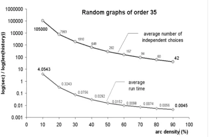
Figure 3: Run time statistics for theAllKernelsprocedure (Algorithm 5)
x contained in its disconnect. This way, Ki+1+ andKi+1− can only contain outranking, re-spectively outranked kernels or stay empty. As we start with empty initial collectionsK0+ andK0−, it is verified that in the endK+, respectivelyK−, if not empty, may only contain outranking, respectively outranked, kernels.
Finally, that the algorithm collects all existing determined outranking and outranked kernels in eG follows from the fact that the strictly-independent-choices graph is strongly connected. Starting in turn from each single choice, the algorithm walks necessarily through all strictly independent choices existing in eG. In order to avoid visiting the same strictly independent choices several times in turn from each member single choice, we keep a history of visited choices and only proceed recursively with the next choiceYi+1 in case it has not yet been visited. 2
Again, using a weak version of the disconnect concept, allows one to extend this algorithm to both, the completely determined as well as the weak kernels.
2.4
Complexity and computational performance
In figure 2.4 we show run times statistics for kernel extractions from randomly filled bipolar-valued digraphs of order 35. Similar to the previous statistics, we find that the extraction of kernels is computationally easy (run times less than a second) when the arc density is 20% and more. Again, the performance is directly related to the order of the
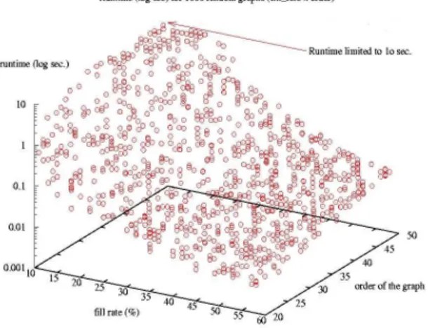
Figure 4: General performance of Algorithm 5
independent-choices graph. Indeed, the higher the arc density, the lower is the order of this choices graph. With an arc density of 50% for instance, we observe an average of only 200 independent choices. We may collect on this choices graph the outranking and outranked kernels in an average of 15 milliseconds on a standard desktop PC.
This run time performance is even better supported in general (see figure 2.4) when considering that almost all digraphs of ordern contain only kernels such that Cn− 1.43 ≤ |K| ≤ Cn+ 2.11 where Cn= ln(n) − ln(ln(n)) (Tomescu [28]). For a randomly filled digraph of order 900 and 50% arc density, we may thus observe kernels of average cardi-nalities of 7. Thus we are able to extract in less than a minute all kernels from digraphs of orders up to 900 and an arc density of 50% and more, under the condition of disposing of a sufficiently large CPU memory. This general performance is most satisfactory, as the particular outranking graphs we are interested in generally represent more or less tran-sitive weak orderings. As empiric studies of random outranking digraphs is confirming, the corresponding digraphs show arc densities always superior to 50% [9]. Nevertheless some digraphs, even of modest order (less than 30), may potentially represent difficult instances. Indeed, as shown in figure 2.4, where we have artificially limited the run time to 10 seconds, a brutal combinatorial explosion appears with digraphs of very low arc density. Here we may easily observe independent choices-graphs of huge exponential size coupled with kernels of cardinalities up ton/2. This definitely limits the practical performance for extracting all kernels from these kinds of digraphs.
for computing kernels in a digraph. Very recently, Alain Hertz1has proposed a pivoting
algorithm which, starting from an arbitrary initial maximal independent choice, visits di-rectly all other existing maximal independent sets in the digraph. This algorithm belongs to the family of reverse searching algorithms such as the simplex algorithm in linear algebra. The pivoting from one maximal independent choice to the other is done in a polynomialO(n) step, such that performances in fact only depend on the actual number of kernels observed in the digraph. Even if this last algorithm is not as efficient as the
AllKernelsprocedure for dense digraps of large orders, it however delivers all kernels for difficult digraphs such as cordlessn-circuits, and n-paths.
All the preceding discussion only concerns the computation of crisp kernels. In the next section we propose an algebraic approach to the same problem via bipolar-valued membership characterisations of choices, which will deliver the necessary algorithms for solving the general bipolar-valued case.
3
Algebraic approach
In this last section we use an early observation by Berge [1, see Chapter 5] concern-ing the fact that kernels in a digraph may be characterised with a specific characteristic functional equation. We extend this idea to the bipolar-valued case with the objective to immediately determine bipolar-valued kernels from the admissible algebraic solutions of these caracteristic equations.
3.1
The kernel characteristic equations
A choiceY in eG(X, eS) may be characterised with the help of bipolar-valued membership assertions eY : X → L, denoting the credibility of the fact that x ∈ Y or not, for all x ∈ X. eY is called a bipolar-valued characterisation of Y , or for short a bipolar-valued choice in eG(X, eS).
Based on the truth-denotation semantics of the bipolar-valued characterisation domain L (see Subsection 1.1), we obtain the following properties:
– eY (x) = +1 signifies that assertion “x ∈ Y ” is certainly true; – eY (x) > 0 signifies that assertion “x ∈ Y ” is more true than false;
– eY (x) = 0 signifies that assertion “x ∈ Y ” is logically undetermined, i.e. could be
either true or false;
– eY (x) < 0 signifies that assertion “x ∈ Y ” is more false than true;
– eY (x) = −1 signifies that assertion “x ∈ Y ” is certainly false. Equivalently, one can say that assertionx /∈ Y is certainly true.
In the following paragraphs, we recall useful results from [8]. They allow us to es-tablish a formal relation with the previous classical subset-based definitions of qualified choices.
Let eY be a bipolar valued characteristaion of a choice in eG(X, eS). We note eY ◦ eS (resp. eY ◦ eS−1) the bipolar-valued matrix productmaxy6=x[min( eY (y), eS(y, x))] (resp. maxy6=x[min(eS(x, y), eY (y))]) for all x, y in X.
Proposition 10
The outranking (resp. outranked) kernels of eG(X, eS) are among the bipolar-valued choices e
Y satisfying the respective following bipolar-valued kernel caracteristic equation systems: e
Y ◦ eS = − eY , (resp. eY ◦ eS−1= − eY ). (13) Proof: Early proofs of this proposition for the Boolean-valued outranked case may be found in [2] and [26; 27]. The classic fuzzy-valued case is tackled in [21], while the bipolar-valued outranking case is thoroughly discussed and proved in [8]. 2
It is worthwhile noting from the beginning, that certain bipolar-valued kernel charac-terisations, despite being different in values, may characterise in fact a same crisp choice. To cope with this phenomena, we introduce the following congruence relation onY, the set of possible characterisations of choices in eG.
We say that two bipolar-valued characterisations ˜Y1 and ˜Y1 of choices in eG are non
contradictory, denoted ˜Y1 ∼= ˜Y2 if and only if ˜Y1(x) > 0 ⇔ ˜Y2(x) > 0 and ˜Y1(x) < 0 ⇔ ˜Y2(x) < 0. Every choice Y in eG determines a congruence class of non contradictory bipolar-valued characterisations denotedY/∼=Y.
Furthermore, it is useful to compare bipolar-valued charaterisations with respect to the sharpness of their charateristic determination.
Definition 14 (Sharpness of bipolar-valued characterisations)
Let ˜Y1, ˜Y2 ∈ Y characterise choices Y in eG. We say that ˜Y1is sharper than ˜Y2, denoted ˜
Y1< ˜Y2if and only if for allx ∈ X, either ˜Y1(x) ≤ ˜Y2(x) ≤ 0, or 0 ≤ ˜Y2(x) ≤ ˜Y1(x). The sharpness relation < determines a partial order onY, the set of possible bipolar-valued characterisations of choices in eG (see [5]). The all 0-valued vector ˜Y (x) = 0, ∀x ∈