Processing and analysis of sounds signals by Huang transform (Empirical Mode Decomposition: EMD)

(1)

HAL Id: tel-00719637

https://tel.archives-ouvertes.fr/tel-00719637

Submitted on 20 Jul 2012

HAL is a multi-disciplinary open access

archive for the deposit and dissemination of sci-entific research documents, whether they are pub-lished or not. The documents may come from teaching and research institutions in France or abroad, or from public or private research centers.

L’archive ouverte pluridisciplinaire HAL, est destinée au dépôt et à la diffusion de documents scientifiques de niveau recherche, publiés ou non, émanant des établissements d’enseignement et de recherche français ou étrangers, des laboratoires publics ou privés.

Processing and analysis of sounds signals by Huang

transform (Empirical Mode Decomposition: EMD)

Kais Khaldi

To cite this version:

Kais Khaldi. Processing and analysis of sounds signals by Huang transform (Empirical Mode Decom-position: EMD). Signal and Image Processing. Télécom Bretagne, Université de Bretagne Occidentale, 2012. English. �tel-00719637�

(2)

N° d’ordre : 2012telb0200

Sous le sceau de l’Université européenne de Bretagne

Télécom Bretagne

En habilitation conjointe avec l’UBO

Ecole Doctorale SICMA

Co-tutelle avec

Ecole Nationale d’Ingénieurs de Tunis

En habilitation conjointe avec l’université Tunis El Manar

Ecole Doctorale STI

TRAITEMENT ET ANALYSE DES SIGNAUX SONORES

PAR TRANSFORMÉE DE HUANG (EMD)

Thèse de Doctorat

Mention : Sciences et Technologies de l’Information et de la Communication

Présentée par Kais Khaldi

Département : Signal et communications

Laboratoire : Lab-STICC

Directeur de thèse : Thierry Chonavel

Soutenue le 20 janvier 2012

Jury

Mme Soﬁa Ben Jebara, Professeur, SUP’COM (Rapporteur)

M. Laurent Daudet, Professeur, Université Paris 7 (Rapporteur)

Mme Amel Ben Azza, Professeur, SUP’COM (Présidente)

M. Ali Khenchaf, Professeur, ENSTA Bretagne (Examinateur)

Mme Monia Turki, MC (HdR), ENIT (Directeur)

(3)

...A mon cher père ...A ma tendre mère.

... A mon épouse et mes fils Ahmed et Ayhem. ...A toute ma famille.

Pour leurs soutiens et sacrifices.

A tous ceux que j’aime et qui m’aiment Et à tout ceux qui m’ont soutenu durant ces années.

(4)

Remerciements

Ce travail a été réalisé conjointement au sein de l’Unité Signaux et Systèmes, de l’Ecole Nationale d’Ingénieurs de Tunis (ENIT), à l’Institut de Recherche de l’Ecole Navale (IRENav) de Brest et au LabSTICC de Télécom Bretagne. En premier lieu, je tiens à exprimer mes remerciements à Madame Soﬁa Ben Jebara, Professeur à SUP’Com et Monsieur Laurent Daudet, Professeur à Uni-versité Paris 7, pour avoir accepté de rapporter cette thèse.

Je remercie Madame Amel Ben Azza, Professeur à SUP’Com et Monsieur Ali Khenchaf, Professeur à ENSTA Bretagne, d’avoir accepté de faire partie du jury.

Je souhaite remercier également Professeur Christophe Claramunt directeur de l’IRENav de m’avoir accueilli et fourni les moyens matériels nécessaires pour mener à bien ce travail pendant mes séjours à l’Ecole Navale. Un grand merci à l’ensemble du groupe ASM de l’IRENav.

J’adresse mes plus vifs et sincères remerciements à mes encadreurs, Madame Monia Turki Maître de Conférence à l’ENIT, Monsieur Thierry Chonavel Pro-fesseur à Télécom Bretagne et Monsieur Abdel-Ouahab Boudraa Maître de Con-férences (HdR) à l’Ecole Navale, pour leur qualité d’encadrement, leur rigueure scientiﬁque, leur soucis permanent de comprendre les problèmes traités ainsi que pour l’ambiance sympatique dans laquelle s’est passée les quatres années. La réussite de ce travail leur revient en grande partie.

Je tiens par ailleurs à remercier Bruno Torrésani Professeur à l’Université de Provence pour l’intérêt qu’il a porté à mes travaux de recherche et pour ses recommandtions et suggestions dans le domaine du codage audio.

(5)

REMERCIEMENTS iii

Je remercie mon épouse, mes parents, mes frères et mes soeurs pour leur soutien et leurs encouragements à surmonter les diﬀérents problèmes rencontrés. Un grand Merci pour tous ceux qui m’ont aidé de prêt ou de loin à réaliser ce travail.

(6)

Résumé détaillé en

français de la thèse

L

a décomposition modale empirique (Empirical Mode Decomposition "EMD" en anglais) est une méthode caractérisée par un processus appelé Tamisage (Sifting) permettant de décomposer temporellement un signal en une somme de composantes oscillantes appelées Modes Empiriques connues sous le nom de Intrinsic Mode Functions (IMF).

Le but général de la thèse est l’exploration des possibilités de l’EMD pour traite-ment et l’analyse des signaux sonores avec comme application débruitage, compres-sion et tatouage. Ainsi, mes travaux de recherche actuels s’inscrivent dans un esprit de continuité du travail eﬀectué en mastère, qui touche particulièrement les traite-ments du signal. Le rapport de la thèse est écrit en anglais, il est structuré en quatre parties.

.1 Transformée de Huang : EMD

Dans ce chapitre, on propose d’étudier la technique EMD en précisant ses caractéris-tiques, tout en insistant sur les critères qui nous oﬀrent une bonne décomposition du signal.

.1.1 Principe de la méthode EMD

L’EMD est une méthode algorithmique de décomposition des signaux. Elle se base sur le principe de décomposer le signal en une somme d’une composante locale haute

(7)

RÉSUMÉ DÉTAILLÉ EN FRANÇAIS DE LA THÈSE v

fréquence (oscillation rapide) et d’une composante basse fréquence (tendance). Ce principe est illustré par l’équation (1):

x(t) = d(t) + m(t) (1)

où x(t) constitue le signal à décomposer, d(t) est l’oscillation rapide, m(t) est le signal tendance et t indique le temps discret.

De même le signal tendance peut être aussi décomposé en deux termes (2).

m(t) = d1(t) + m1(t) (2)

où d1(t) est la composante haute fréquence et m1(t) est la composante basse

fréquence.

Pour calculer un mode relatif à un signal, on suit le principe suivant : 1. Identiﬁer tous les extrema locaux de x(t).

2. Interpoler les minima (resp. les maxima) de manière à construire une certaine enveloppe: EnvMin (resp. EnvMax).

3. Calculer la moyenne de deux enveloppes m(t) = ( EnvMin(t) + EnvMax(t))/2. 4. Extraire le détail d(t) = x(t) − m(t). Le signal d(t) n’est consideré IMF qu’après un certains nombre d’itérations nécessaires aﬁn que d(t) obéisse à un critère d’arrêt donné.

En itérant ce principe, on obtient une décomposition du signal décrite comme suit: x(t) = N X j=1 IMFj(t) + r(t) avec N ∈ N∗ (3)

où IMFj est l’IMF d’ordre j qui est de type plus haute fréquence que l’IMFj+1.

Le signal r(t) est appelé résidu, il correspond à la composante la plus basse fréquence du signal.

(8)

RÉSUMÉ DÉTAILLÉ EN FRANÇAIS DE LA THÈSE vi

original sans perte ou distorsion de l’information [34].

Toutefois, on ne parle d’une IMF que si elle vériﬁe les critères suivants [34]: 1. Une moyenne nulle.

2. La diﬀérence entre le nombre d’extrema et le nombre de passage à zéros est au plus de un (c’est à dire qu’entre un minimum et un maximum successif, l’IMF passe par zéro).

Le principe de décomposition de l’EMD est assuré par le processus de tamisage déﬁni par l’algorithme décrit dans ce qui suit.

.1.2 Procédure algorithmique de l’EMD

Notations :

ǫ: indique le seuil prédéﬁnie, c’est un critère de condition de la boucle indicée par i.

j : représente l’indice de l’IMF.

i : constitue l’indice de l’itération appliquée sur le résidu pour vériﬁer le critère d’une IMF.

rj : désigne le résidu aprés l’obtention de la jeme IMF

hj,i : c’est une variable intermédiaire de calcul qui prend la valeur du nouveau

résidu à la première itération, puis, elle prend la diﬀérence entre le résidu et la valeur de l’enveloppe moyenne aux itérations suivantes.

Uj,i: représente l’enveloppe supérieure de hj,i, construite par interpolation des

maxima.

Lj,i : représente l’enveloppe inférieure de hj,i, construite par interpolation des

minima.

µj,i : désigne l’enveloppe moyenne, obtenu à partir des deux enveloppes de hj,i.

SD (i) : indique le critère d’arrêt à la ième _itération.

L’algorithme correspondant à la méthode EMD peut s’écrire sous la forme du pseudo - code suivant :

Etape1: ﬁxer ǫ, j ← 1 (jème_IMF_).

Etape2 : rj₋₁(t) ← x(t) (résidu).

Etape3 : extraire la jème_IMF _:

(a) : hj,i−1(t) ← rj−1(t) ,i ← 1 ( i;itération de la boucle sifting).

(9)

RÉSUMÉ DÉTAILLÉ EN FRANÇAIS DE LA THÈSE vii

(c) : calculer les enveloppes supérieure et inférieure : Uj,i−1(t) et Lj,i−1(t) par

in-terpolation ( splines cubiques par exemple ) des maxima et des minima de hj,i₋₁(t)

respectivement.

(d) : calculer l’enveloppe moyenne : µj,i₋₁(t) =(Uj,i₋₁(t) + Lj,i₋₁(t))/2.

(e) : mettre à jour hj,i(t) ← hj,i−1(t)- µj,i−1(t) , i ← i + 1.

(f) : calculer le critère d’arrêt (par exemple) : SD(i) =

T

X

t=0

|hj,i−1(t)−hj,i(t)|2

(hj,i−1(t))2 ,

où T représente le nombre d’échantillons du signal.

(g) : décision : répeter l’étape (b),(f) tant que SD(i)<ǫ.

à la sortie de l’étape(3), on met IMFj ← hj,i(t) (jèmeIMF).

Etape4 : mettre à jour le résidu rj(t) ← rj−1(t) - IMFj(t).

Etape5 : répéter l’étape(3) avec j ← j + 1 jusq’u à ce que le nombre d’extrema

dans rj(t) ≤ 2.

L’algorithme décrit ci-dessus, comporte deux boucles imbriquées l’une dans l’autre, celle indicée par j permet d’extraire l’IMF, qui nous détermine le niveau de pro-fondeur de décomposition et l’autre indicée par i conditionne la fonction IMFj(t) de manière à respecter les critères requis; avoir deux enveloppes symétriques aﬁn que le signal extrait IMFj soit bien une IMF.

Une bonne décomposition donnée par cet algorithme est conditionnée par le choix de certains paramètres.

.1.3

Paramètres pertinants de la décomposition

Généralement, le choix des paramètres repose sur le critère d’arrêt. Comme il existe deux boucles dans l’algorithme, il faut s’assurer que les deux doivent s’arrêter. La boucle principale indicée par j s’arrête lorsqu’il n’est plus possible de décomposer le résidu courant càd que rj(t) possède moins de deux extrema. La boucle indicée

par i est liée à un critère d’arrêt qu’il convient de déﬁnir de manière précise. La 2`eme _{boucle (indicée par i) va s’arrêter lorsque h}

j,i(t) vériﬁe les critères de

définition d’une IMF ( de moyenne nulle). Théoriquement, cette hypothèse n’est pas démontrée, pour cela en pratique on ajoute à ce critère un autre qui évite au proccesus de tamisage entrer dans une boucle infinie. La définition d’un critère d’arrêt du processus de tamisage est alors nécessaire:

(10)

RÉSUMÉ DÉTAILLÉ EN FRANÇAIS DE LA THÈSE viii

deviation standard et déﬁni par :

SD(i) = T X t=0 |hj, i − 1(t) − hj, i(t)|2 (hj, i − 1(t))2 (4)

Le test d’arrêt est validé lorsque la différence entre deux tamisages consécutifs est inférieur à un seuil prédéfinie ǫ. Typiquement, la valeur ǫ permettant de stopper le tamisage est comprise entre 0.2 et 0.3 [1]. Cette valeur réalise un certain compromis. En effet si ǫ est trop grand, l’EMD ne permet pas de séparer les différents modes présents dans le signal, cependant si ǫ est trop petit, l’EMD risque d’aboutir a des composantes dont l’amplitude est quasiment constante et modulée par une seule fréquence ( sur-décomposition de signal).

Un autre critère local a été proposé par P.Flandrin [28] et notamment choisi en pratique. Ce critère est déﬁni comme suit :

σ(t) = 2| µi−1(t) Ui₋₁(t) − Li₋₁(t)|

(5) En adoptant le critère σ(t), trois conditions nécessaires sont déﬁnies pour que hi,j(t) soit bien une IMF [28].

• La diﬀérence entre le nombre de zéros de hi(t) et les nombres d’extrema de

hi(t) est infèrieure ou égale en valeur absolue à 1.

• σ(t) < θ1 pour t ≤ (1 - α)T

• σ(t) < θ2 pour (1 - α)T < t <T

où T : la taille de la fenêtre d’analyse, θ1et θ2 deux réels tels que 0 ≤ θ1 ≤ θ2 et

0 ≤ (α ≡ (T olerence)) ≤1

La première condition revient à dire qu’une IMF doit être une fonction oscillante autour de zéro : entre un maximum et un minimum, il doit y avoir un passage par zéro. Les deux dernières conditions exigent que le paramètre σ(t) soit faible. Toute fois, il peut dans une certaine mesure prendre des valeurs élevées.

Dans [28]le bon copromis du choix des valeurs des seuils θ1et θ2 est le suivant :

θ1 ≈ 0.05 et θ2 ≈ 10 ∗ θ1 et α ≈ 0.05. On conclut que tous les critères d’arrêt

(11)

RÉSUMÉ DÉTAILLÉ EN FRANÇAIS DE LA THÈSE ix

Dans notre travail, nous adoptons le critère choisie par [28], car il nous permet d’obtenir des modes qui correspondent bien à la déﬁnition d’une IMF.

.2 Débruitage des signaux de la parole par EMD

Nous présentons dans cette partie une procédure basée sur l’EMD pour le rehausse-ment du signal de la parole. En particulier le traiterehausse-ment proposé tiendra compte du caractère voisé ou non voisé de la séquence de parole considérée. Puisque le signal de parole est constitué de séquences voisées et non voisées, on a été amené à considérer séparément les deux types de séquences.

L’idée du débruitage d’un signal de parole bruité se présente selon le principe suivant: 1. Découper le signal bruité en trames.

2. Pour chaque trame on fait appelle à l’EMD pour la décomposer.

3. Après avoir décomposer la trame bruitée en modes, on calcule l’énergie de cha-cun des modes et suivant la variation des énergies, on déduit le type de la trame.

4. Suivant le type de la trame, on applique le procédé du débruitage, c’est à dire s’il s’agit d’une séquence voisée, on applique l’approche du ﬁltrage puis on débruite seulement les modes qui ne sont pas pris lors du ﬁltrage par EMD, alors que dans le cas d’une séquence non voisée, on débruite tous les modes.

5. Le signal estimé est reconstruit en utilisant les séquences débruitées.

.2.1

Débruitage de séquences voisées

La séparation entre le bruit et le signal original est possible. En fait, cette sépa-ration se base sur l’hypothèse que les premières IMF (les modes de plus hautes fréquences) sont majoritairement dominés par le bruit et sont peu représentatives de l’information propre au signal initial. Cependant, les modes qui correspondent au signal non bruité contiennent quand même un peu du bruit. Le débruitage de ces modes va engendrer une distorsion au niveau de reconstitution du signal es-timé. Ainsi, le débruitage d’une séquence voisée revient à débruiter seulement les modes qui ne sont pas ﬁltrés par EMD. Enﬁn, le signal débruité est la somme des

(12)

RÉSUMÉ DÉTAILLÉ EN FRANÇAIS DE LA THÈSE x

modes ﬁltrés par EMD et les modes débruités. L’approche proposée est résumée par l’organigramme suivant:

Séquence bruitée ✲ _EMD ✲

✲ ✲ ✲ ✲ ✲ ✲ ✲ MMSE MMSE MMSE MMSE + ✇ ❘ ⑦ ③ ✲ ✯✸❃ Séquence estimée Résidu IMFN IMFN−1 IMFK IMFk−1 IMF3 IMF2 IMF1 ✰ Critère énergétique ✲

Organigramme de débruitage d’une séquence voisée par approche EMD-MMSE

.2.2

Débruitage de séquences non voisées

Lors de la décomposition d’un signal de type non voisé bruité par EMD, qu’il est difficile de séparer le signal original du bruit. Cependant, l’hypothèse que le bruit est uniquement réparti sur les premières IMF n’est pas vérifiée sur les séquences non voisées. Ainsi, les informations qui correspondent au signal original seraient intégrées dans tous les modes, donc l’approche du débruitage se basera sur un traitement de tous ces modes un par un. La procédé consiste à reconstruire le signal estimé avec toutes les IMF préalablement filtrés.

(13)

RÉSUMÉ DÉTAILLÉ EN FRANÇAIS DE LA THÈSE xi

.3 Codage des signaux audio par EMD

Dans cette partie, nous proposons une alternative à la décomposition par ondelettes, il s’agit de la décomposition modale empirique (EMD) [34]. Contrairement à la décomposition par ondelettes, l’EMD est entièrement pilotée par les données. Par conséquent, l’EMD ne nécessite pas le choix a priori d’une famille de fonctions de base de décomposition des signaux.

L’EMD consiste à décomposer un signal en une somme finie d’IMF. L’analyse du processus du tamisage qui génère les IMF montre qu’on peut envisager un schéma de compression à bas débit basé sur le codage des IMF du signal audio à coder. En effet, chaque IMF peut être vue comme la composante du signal dans une certaine sous-bande, implicitement définie par l’EMD [28]. Du fait du caractère oscillant et de moyenne nulle des signaux à bande étroite, le codage de chaque IMF peut être réalisé en ne considérant que ses extrema. Notons, en particulier qu’une simple interpolation de ses extrema au moyen de fonctions spline[47], permet la la reconstruction presque parfaite de l’IMF considérée. L’analyse du processus du tamisage qui génère les IMF montre qu’on peut envisager un schéma de compression des signaux à bas débit en utilisant l’approche EMD. En effet, comme chaque IMF est représentée uniquement par ses extrema et un modèle d’interpolation spline, un codage pour la compression est possible. Ainsi, la compression du signal correspond à celle des extrema des IMF. Donc, le décodeur aura besoin uniquement des extrema préalablement stockés pour reconstruire les IMF et par conséquent le signal initial. L’association du modèle psycho-acoustique dans le procédé de codage des extrema des différents IMFs obtenus, garantira une bonne qualité d’écoute du signal décodé. La nouvelle technique est décomposée en plusieurs modules liés les uns aux autres. Le principe de l’approche proposée est résumé par l’organigramme de la Figure 1.

.3.1 Décomposition par EMD

On découpe tout d’abord le signal audio en trames de taille 512 échantillons [63]. En utilisant le processus de tamisage, chaque trame du signal est ensuite décom-posée temporellement en une somme de composantes modales (IMFi)i=1,C, qui sont

(14)

RÉSUMÉ DÉTAILLÉ EN FRANÇAIS DE LA THÈSE xii ❄ ❄ Extraction d’extrema ❄ ❄ Seuillage ❄ ❄ Quantiﬁcation Code de Huﬀman ❄ EMD ❄ IMF1 . IMF_C . . . . . . . . E1,1 EC,1 E1,N 1 EC,N n . . . . Signal codé (Trame codée) Signal e1,1 eC,1 e1,n1 eC,nn . . . . Modèle Psycho-acoustique ❄ ✛ ✛ ✻ (Trame)

Figure 1: Organigramme de la compression par EMD.

complètement représentées par leurs extrema (Ei,Ni)i=1,C, avec Ea,b = (Xa,b, Ya,b) la

position du bème _{extremum de l’IMF a.}

.3.2 Seuillage des extrema selon le modèle

psycho-acoustique

Notre objectif dans cette partie est de réduire au maximum le nombre d’extrema d’une IMF, tout en assurant que l’erreur entre l’IMF estimée à partir des extrema restants et la vraie IMF reste au-dessous de son seuil de masquage. Ce dernier est calculé en se basant sur le modèle psycho-acoustique utilisé dans le codeur MPEG1. La technique de seuillage utilisée ici est de type dur [55]. On obtient ainsi un jeux réduit d’extrema (ei,ni)i=1,C.

(15)

RÉSUMÉ DÉTAILLÉ EN FRANÇAIS DE LA THÈSE xiii

.3.3 Quantification des extrema seuillées

Puisque le nombre des extrema seuillés décroît d’une IMF à la suivante (les IMF successives sélectionnent des composantes du signal de fréquences de plus en plus basses), le nombre de bits alloués varie d’une IMF à l’autre aﬁn d’optimiser l’allocation de débit, comme c’est le cas dans les codeurs en sous-bandes de type MPEG. Ainsi, le nombre réduit de bits utilisés pour coder les extrema de chaque IMF doit garantir l’inaudibilité de l’erreur de quantiﬁcation de l’IMF.

Pour cela, on commence par affecter un même nombre réduit de bits pour chaque IMF. Ce nombre de bits peut être ensuite augmenté jusqu’à assurer l’inaudibilité de l’erreur de codage de l’IMF. Il s’agit d’un procédé itératif de quantification de l’IMF suivi de sa reconstruction, en augmentant progressivement le nombre de bits alloués jusqu’à satisfaire la contrainte de masquage. En fait, ce procédé consiste à quantifier l’IMF, la reconstruire puis comparer la Densité Spectrale de Puissance (DSP) son erreur par rapport à son seuil de masquage. Si la DSP de l’erreur est au dessus du seuil de masquage, on recommence la quantification en augmentant le nombre de bits alloués et ainsi de suite jusqu’à ce que la DSP de l’erreur soit au dessous de la courbe de masquage.

Au début, on ﬁxe le nombre de bits pour tout extrema des IMFs (1 bits), la mise à jour du nombre de bits est obtenue en addition par un l’ancienne valeur du nombre de bits. Dés que la nouvelle IMF reconstruite respecte le seuil de masquage, la boucle de quantiﬁcation pour cette IMF s’arrête.

Cette méthode de quantiﬁcation présente un avantage, car le nombre de bits utilisés pour respecter la contrainte psycho-acoustique est ici minimisé individuellement pour chaque IMF.

.3.4 Codage

La réduction de l’information redondante résiduelle est alors assurée par un codage d’Huﬀman. Son principe est basé sur une étude statistique déﬁnie par la PDF (Probability Density Function) . Le code le plus fréquent est attribué à un nouveau code contenant le nombre minimal des bits possible et ainsi de suite.

(16)

RÉSUMÉ DÉTAILLÉ EN FRANÇAIS DE LA THÈSE xiv

.3.5 Résultats de simulation

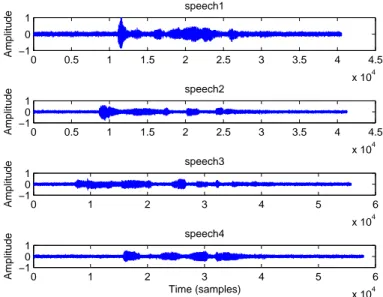
L’approche de la compression par EMD est appliquée à des signaux audio de natures diﬀérentes (chanson, guitare, piano et violon). Ils sont tous échantillonnés à la même fréquence fe = 44.1KHz. La Figure 2 présente les signaux originaux. Chaque signal est découpé en trames de taille 512 échantillons [63]. Ensuite en utilisant le processus de tamisage, chaque trame du signal est decompsée en ensembles d’IMFs et un résidu. Les positions des extrema sont codés sur 9 bits, alors que leurs valeurs sont codés selon le procédé de quantiﬁcation décrit ci-dessus.

0 0.5 1 1.5 2 2.5 3 3.5 4 4.5 x 104 −1 0 1 Amplitude guitare 0 0.5 1 1.5 2 2.5 3 3.5 4 4.5 x 105 −1 0 1 Amplitude chanson 0.5 1 1.5 2 2.5 3 3.5 4 x 104 −1 0 1 Amplitude piano 1 2 3 4 5 6 x 105 −1 0 1 Temps ( en échantillons) Amplitude violon

Figure 2: Signaux audio (chanson, guitare, piano et violon)

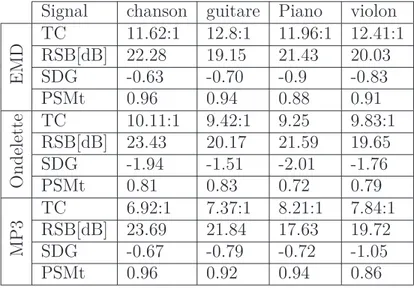
Les résultats obtenus par la méthode proposée sont comparés à ceux obtenus par la méthode à base de l’ondelette (Daubechies 8) [20] et le codeur MP3 [?]. En fait, nous avons choisi db8 de 5 niveaux de décomposition, parce qu’elle donne de meilleurs résultats par rapport aux autres types d’ondelettes [20]. Comme critère d’évaluation des performances de la compression des signaux audio, nous avons opté pour le Taux de Compression (TC), Rapport Signal à Bruit (RSB), Subjective Difference Grade (SDG) et instantaneous Perceptual Similarity Measure (PSMt). Ces deux derniers critères sont offrent une évaluation de la qualité d’écoute du signal. subjective Les valeurs de TC, RSB, SDG et PSMt obtenues par ces différentes méthodes sont présentées dans le tableau VI.1.

(17)

RÉSUMÉ DÉTAILLÉ EN FRANÇAIS DE LA THÈSE xv

Table 1: Résultats de la compression par EMD, MP3 et par ondelette. Signal chanson guitare Piano violon

E M D TC_{RSB[dB] 22.28}11.62:1 12.8:1_19.15 11.96:1 12.41:1_21.43 _20.03 SDG -0.63 -0.70 -0.9 -0.83 PSMt 0.96 0.94 0.88 0.91 O nd el et te TC 10.11:1 9.42:1 9.25 9.83:1 RSB[dB] 23.43 20.17 21.59 19.65 SDG -1.94 -1.51 -2.01 -1.76 PSMt 0.81 0.83 0.72 0.79 M P 3 TC_{RSB[dB] 23.69}6.92:1 7.37:1_21.84 8.21:1_17.63 7.84:1_19.72 SDG -0.67 -0.79 -0.72 -1.05 PSMt 0.96 0.92 0.94 0.86

que celles des autres techniques testées. En eﬀet, l’analyse des valeurs du TC et du (SDG) montre qu’elle oﬀre une amélioration en termes de taux de compression et de qualité audio du signal décodé respectivement. En particulier cette amélioration est clairement visible surtout pour les signaux guitare et violon.

.4 Tatouage des signaux audio par EMD

L’EMD consiste à décomposer un signal en une somme ﬁnie de composantes de type AM-FM, appelées IMF (Intrinsic Mode Function). L’analyse du processus du tamisage qui génère les IMF montre qu’on peut envisager un schéma de tatouage qui consiste à insérer la marque dans la dernière IMF. En eﬀet, la dernière IMF peut être vue comme la composante la plus basse fréquence, par conséquence la plus résistante aux attaques. Ainsi, on propose d’insérer la marque en association avec le code de synchronisation dans les extrema de la dernière IMF.

.4.1 Algorithme de tatouage proposé

Code de synchronisation

Le code de synchronisation est introduit pour localiser la position de la marque dans le signal et par conséquence facilite l’extraction de la marque du signal tatoué.

(18)

RÉSUMÉ DÉTAILLÉ EN FRANÇAIS DE LA THÈSE xvi

Etant donné un code de sunchronisation U et une séquence inconnue V qui sont de même longeur. La séquence V est déﬁnie comme étant un code de synchronisation si seulement la valeur de simularité entre U et V (bit par bit) est supérieur ou égale à un seuil prédeﬁni τ.

Procédure d’insertion

Après combination de la marque avec le code de synchronisation pour former un ﬂux binaire mi, la procédure d’insertion de la marque est illustré dans les étapes

suivantes:

Etape 1: Segmenter le signal audio en trames.

Etape 2: Decomposer chaque trame en IMFs, en utilisant l’EMD.

Etape 3: Insérer P fois la séquence binaire mi dans les extrema de la dernière IMF.

L’insertion des bits se fait par modulation d’amplitude des extrema, ainsi chaque bit de sequence binaire doit être inséré comme suit:

e′i =    ⌊ei/S⌋.S sgn 3S/4 si mi = 1 ⌊ei/S⌋.S sgn S/4 si mi = 0 (6)

ei et e′i désigne les extrema de la dernière IMF de signal audio respectivement le

signal audio tatoué. sgn est égale à "+" si ei est un maximum, et "-" si’il est un

minimum. ⌊ ⌋ est la fonction partie entière, et S répresente le facteur d’insertion, que doit être choisi de telle sorte que le signal tatoué respecte la contraine d’inaudibilité.

Etape 4: Reconstruire la trame (EMD-1_{) en utilisant la dernière IMF modiﬁée puis}

on concaténe la trame tatouée pour construire le signal audio tatoué.

Procédure d’extraction

Etant donné N1 et N2 est le nombre de bits de code de synchronisation

respective-ment le nombre de bits de la marque. L’extraction de la marque est décrit comme suit:

Etape 1: Segmenter le signal en trames.

Etape 2: Decomposer chaque trame en IMFs, en utilisant l’EMD. Etape 3: Extracter les extrema e∗

(19)

RÉSUMÉ DÉTAILLÉ EN FRANÇAIS DE LA THÈSE xvii

Etape 4: Extracter la sequence m∗

i de e∗i. m∗i =    1 si e∗ i − ⌊e∗i/S⌋.S ≥ sgn S/2 0 si e∗ i − ⌊e∗i/S⌋.S < sgn S/2 (7) sgn est "+" si e∗

i est un maximum,et "-" s’il est un minimum.

Etape5: Grouper toute sequence de bits yi.

Etape 6: I ← 1 et L ← N1 (taille fenêtre)

Etape 7: Evaluer la similarité entre le premier code de synchronisation extracté,

V = y(I:L), et le code de synchronisation original U bit par bit. Si la valeur de similarité est ≥ τ, Donc V est considéré comme étant le code de synchronisation et sauter à l’étape 9, sinon aller à l’étape 8.

Etape 8: I ← I + 1 et L ← L + 1 et revenir à l’étape 7.

Etape 9: Evaluer la similarité entre le second code de synchronisation extracté,

V’=y(I+N1+N2: I+2N1+N2) et le code de synchronisation original. si la valeur de

similarité ≥ τ, donc V′ _{est considéré comme étant le code de synchronisation code,}

et extracter la marque N2 bits (y(I+N1: I+N1+N2-1)) à partir de la position I+N1

et aller à l’étape 10, sinon revenir à l’étape 8.

Etape 10: I ← I +N1+N2, si la nouvelle valeur I est égale à la longeur de séquence

yi, aller à l’étape 11, sinon revenir à l’étape 8.

Etape 11: Extracter le P marques et fait comparison bit par bit entre ces marques,

pour la correction, et ﬁnalement extracter la marque désirée.

.4.2 Principaux résultats

Pour illustrer les performances de l’algorithme de tatouage par EMD, nous avons eﬀectué des simulations numériques sur des signaux audio de natures diﬀérentes. Les signaux sont tous échantillonnés à la fréquence fe = 44.1KHz. La marque est une image logo binaire.

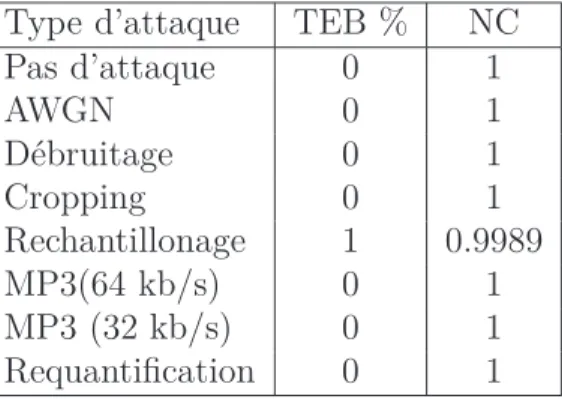
Pour evaluer la performance de l’algorithme proposé, nous avons utilisé les deux critères suivants : TEB et NC (Normalised Cross-correlation).

Table VI.1 montre la robustesse de l’algoritme proposé pour le signal audio "Rock". Les Valeurs de TEB et NC reﬂette la bonne performance de notre algorithme pour diﬀerents type d’attaques.

Le tableau B.1 montre que notre approche présente de meilleures performances que les autres techniques testées. En eﬀet, elle oﬀre une amélioration en termes de débits et robustesse en fonction de codeur MP3 par rapport aux autres algorithmes

(20)

RÉSUMÉ DÉTAILLÉ EN FRANÇAIS DE LA THÈSE xviii

Table 2: TEB et NC de la marque extractée pour le signal audio "Rock" par l’approche proposée.

Type d’attaque TEB % NC Pas d’attaque 0 1 AWGN 0 1 Débruitage 0 1 Cropping 0 1 Rechantillonage 1 0.9989 MP3(64 kb/s) 0 1 MP3 (32 kb/s) 0 1 Requantiﬁcation 0 1 de tatouage.

Table 3: Performance des algorithmes de tatouage, trier par débits. Référence Débits (b/s) Robustesse avec MP3 (kb/s) Algorithme proposé 46.9-50.3 32 Bhat K 45.9 32 Lie 43 80 Cvejic 27.1 32 Yeo 10 96 Tachibana 8.5 96 Li 4.2 32 Mansour 2.3 56 Xiang 2 64 Kirovski 0.5-1 32

.5 Conclusion

Dans cette thèse on a exploré l’apport de l’EMD en traitement et en analyse des signaux audio et de parole. Cette décomposition du signal en IMF est adaptative et ne fait pas d’hypothèses (stationnarité et linéarité) sur le signal à analyser. Le comportement en banc de ﬁltre dyadique de l’EMD ainsi que la quasi-symétrie des modes et leur représentation via leurs extrema sont les propriétés qui sont l’origine des outils qu’on a développés: débruitage, codage et tatouage. Ces contributions sont illustrées sur des données synthétiques et réelles et les résultats comparés à ceux de méthodes éprouvées telles que le ﬁltre MMSE, l’approche ondelettes et les codecs AAC et MP3 montrent les bonnes performances des outils développés autour de l’EMD. Ces résultats montrent les capacités de l’EMD comme outils de traitement et d’analyse de façon adaptative des signaux audio et de parole.

(21)

CONTENTS 2 List of Figures 6 List of Tables 11 Abbreviations 14 Introduction 15 I Huang transform 24 I.1 Introduction . . . 25 I.1.1 Principle of EMD . . . 25 I.1.2 EMD algorithm . . . 26 I.1.3 Meaningful parameters of EMD . . . 27 I.1.3.1 Stopping criterion . . . 28 I.1.3.2 Interpolation . . . 29 I.2 IMFs properties . . . 31 I.2.1 IMFs orthogonality . . . 31 I.2.2 PDE for IMFs characterization . . . 33 I.3 EMD: a time-frequency description tool . . . 33 I.3.1 Importance of the sampling frequency . . . 33 I.3.2 Tones separation . . . 35 I.3.3 EMD acts as a Filter bank: Gaussian white noise case . . . 37 I.3.4 Comparison with wavelets . . . 38 I.4 Conclusion . . . 40

II Speech enhancement by EMD 42

II.1 Introduction . . . 43 II.2 EMD based white noise reduction . . . 43 II.2.1 EMD-MMSE ﬁlter . . . 44 II.2.2 EMD-Shrinkage . . . 45 II.2.3 EMD-MMSE versus EMD-Shrinkage . . . 46

(23)

CONTENTS 3

II.3 EMD-ACWA ﬁltering of white and colored noises . . . 50 II.3.1 Interest of ACWA ﬁlter . . . 50 II.3.2 Performance analysis of EMD-ACWA . . . 54 II.4 Conclusion . . . 59

III Speech denoising using EMD and local statistics 63

III.1 Introduction . . . 65 III.2 Frames classiﬁcation . . . 65 III.2.1 Voiced frames detection . . . 66 III.2.2 Transient frames detection . . . 68 III.3 Proposed speech denoising method . . . 70 III.3.1 Voiced sequence denoising . . . 72 III.3.2 Unvoiced sequence denoising . . . 73 III.3.3 Transient sequence denoising . . . 73 III.4 Performance analysis . . . 73 III.4.1 Voiced frames . . . 73 III.4.2 Speech signal . . . 78 III.5 Conclusion . . . 82

IV Signal coding schemes in EMD framework 85

IV.1 Introduction . . . 87 IV.2 Why IMFs coding? . . . 87 IV.2.1 IMF extrema . . . 87 IV.2.2 Quasi-symmetry of IMF . . . 88 IV.2.3 IMF modelling . . . 89 IV.3 EMD based encoder architecture . . . 90 IV.3.1 IMF extrema coding basics: IMFextrema . . . 90

IV.3.1.1 Segmentation and decomposition . . . 90 IV.3.1.2 Extrema thresholding . . . 90 IV.3.1.3 Extrema quantiﬁcation . . . 91

(24)

CONTENTS 4

IV.3.1.4 Coding . . . 92 IV.3.1.5 Decoding process . . . 92 IV.3.2 IMF envelope coding basics : IMFenvelope. . . 92

IV.3.2.1 Encoding scheme . . . 92 IV.3.2.2 Decoding process . . . 93 IV.4 HHT based encoder architecture . . . 94 IV.4.1 IA and IP coding basics: IA − IP . . . 94 IV.4.1.1 IA encoding . . . 94 IV.4.1.2 IP encoding . . . 94 IV.4.1.3 Decoding scheme . . . 94 IV.4.2 IA and IF coding basics: IA − IF . . . 95 IV.4.2.1 IF encoding . . . 95 IV.4.2.2 Decoding approach . . . 96 IV.5 conclusion . . . 96

V Encoding schemes: Application to audio signals 99

V.1 Introduction . . . 100 V.2 Encoders architecture . . . 100 V.2.1 Transient detection . . . 100 V.2.2 Thresholding step for IMFextrema coder . . . 103

V.2.3 Quantization step for IMFenvelope and IMFextrema . . . 104

V.3 EMD based audio coders performance . . . 105 V.4 Conclusion . . . 108

VI Audio watermarking based on the EMD 110

VI.1 Introduction . . . 112 VI.2 Proposed watermarking algorithm . . . 112 VI.2.1 Synchronization code . . . 114 VI.2.2 Watermark embedding . . . 115 VI.2.3 Watermark extraction . . . 116

(25)

CONTENTS 5

VI.3 Performance analysis . . . 117 VI.4 Results . . . 118 VI.5 Conclusion . . . 124

Conclusion and perspectives 126

Bibliography 132

Appendix 141

A Chapter III 141

(26)

List of Figures

1 Organigramme de la compression par EMD. . . xii 2 Signaux audio (chanson, guitare, piano et violon) . . . xiv I.1 Interpolation of the signal (x(t) = cos(t)+q

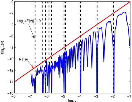
(t)) by diﬀerent methods and the corresponding error. . . 30 I.2 Decomposition the signal x(t) = sin(8t) + sin(3t) + 2t by EMD. . . . 31 I.3 Decomposition of the tone signal (Eq. I.13) by EMD. . . 34 I.4 Estimation and behavior of E(ν) associated with the ﬁrst IMF for a

tone. . . 35 I.5 Decomposition of the signal (Eq.I.15) by EMD. . . 36 I.6 Estimation and behavior of the error E(ν1, ν2) Eq. I.16 for signal

x(t) = xν1(t) + xν2(t) = cos(2πν1t) + cos(2πν2t). . . 37

I.7 IMFs spectra for a white noise. . . 38 I.8 Signal x(t) = sin(3t) + sin(0.3t) + sin(0.03t) and its theoretical

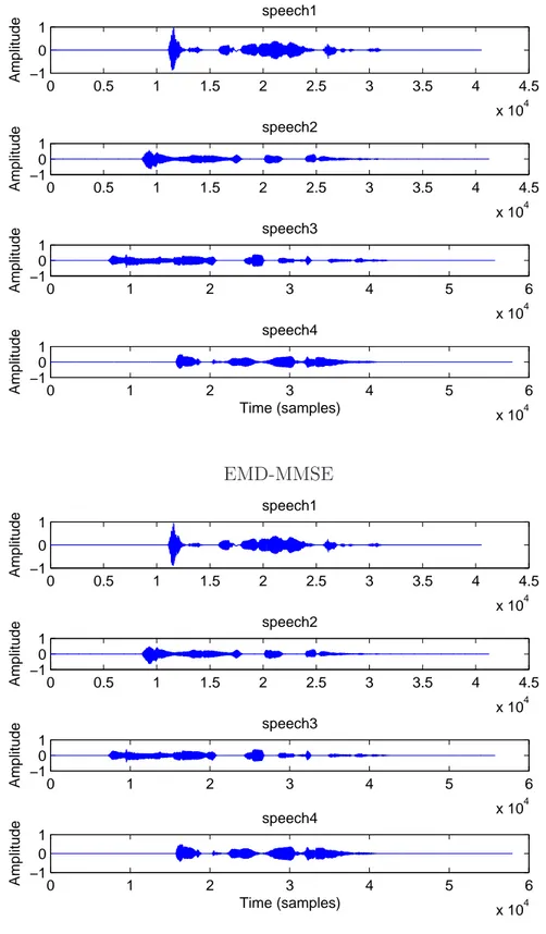
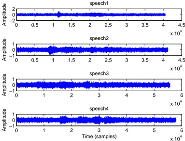
com-ponents. . . 39 I.9 Comparison of decomposition by the EMD to wavelet. . . 39 I.10 Error estimates with EMD and wavelet. . . 40 II.1 Original signals "speech1", "speech2", "speech3" and "speech4". . . 46 II.2 Noisy version of signals "speech1", "speech2","speech3" and "speech4"

(input SNR = 5 dB). . . 47 II.3 Denoising results of signals "speech1", "speech2","speech3" and

(27)

LIST OF FIGURES 7

II.4 Final SNR values obtained from different initial noise levels of signals "speech1", "speech2", "speech3" and "speech4". The results are aver-ages over 100 instances of the noisy signals. They are reported for EMD-MMSE and the MMSE filter. . . 49 II.5 PESQ values obtained from different initial noise levels of signals

"speech1", "speech2", "speech3" and "speech4". The results are aver-ages over 100 instances of the noisy signals. They are for EMD-MMSE and the MMSE ﬁlter. . . 50 II.6 Noisy versions of signals "speech1", "speech2", "speech3" and "speech4"

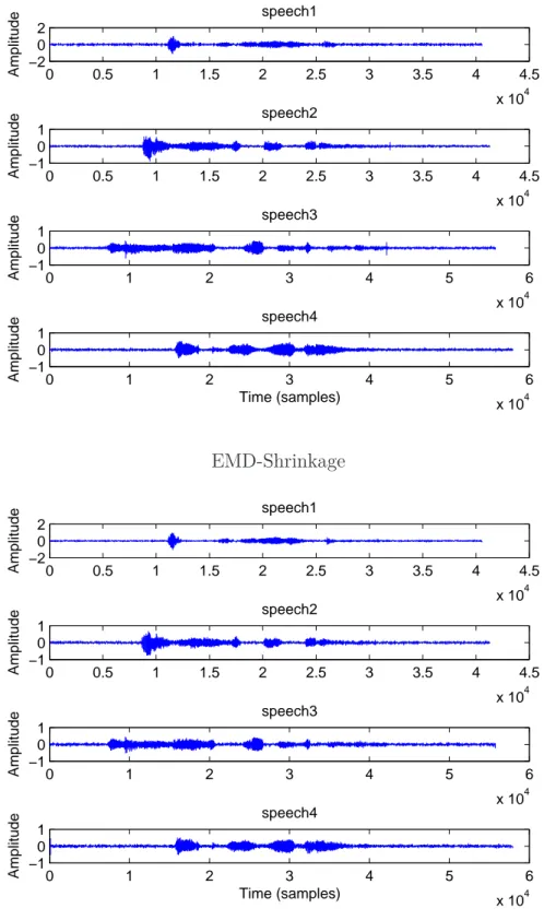
(input SNR =-5 dB). . . 51 II.7 Denoising results of signals "speech1", "speech2", "speech3" and

"speech4" by the EMD-Shrinkage and the wavelet approach (Daubechies 4). . . 52 II.8 Final SNR values obtained from diﬀerent initial noise levels of signals

"speech1", "speech2", "speech3" and "speech4". The results are aver-ages over 100 instances of the noisy signals. They are reported for EMD-Shrinkage and for three diﬀerent Wavelets (Haar, Symmlet 4, Daubechies 4). . . 53 II.9 Variations of the PESQ values versus from the input SNR for signals

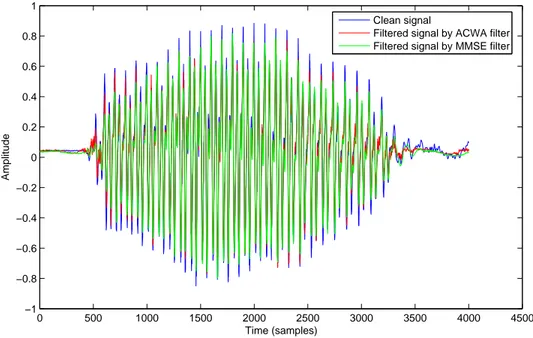
"speech1", "speech2", "speech3" and "speech4". The results are aver-ages over 100 instances of the noisy signals. They are reported for EMD-Shrinkage and for three different wavelets (Haar, Symmlet 4, Daubechies 4). . . 54 II.10 Clean and filtered signals by the ACWA and the MMSE filters (input

SNR=2 dB). . . 55 II.11 Noise power spectral density . . . 56 II.12 Original signals ("speech1" and "speech2") and their noisy versions

(f16 noise with SNR =-2 dB). . . 56 II.13 Variation of the output SNR relating to the noisy signal "speech1"

versus the size L of the ACWA ﬁlter window (f16 noise with SNR=-2 dB and SNR=0 dB). . . 57

(28)

LIST OF FIGURES 8

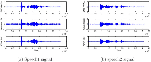
II.14 Denoised version of the signals "speech1" and "speech2" obtained by the EMD-ACWA, the wavelet (db4) and ACWA ﬁlter (f16 noise with input SNR =-2 dB) . . . 58 II.15 Variation of the output SNR versus the input SNR relating to the

denoising of the signals "speech1" and "speech2" corrupted by a white Gaussian noise. The results are averages over 100 instances of the noisy signals. They are reported for EMD-ACWA, ACWA ﬁlter and wavelet(db4) . . . 58 II.16 Variation of the output SNR versus the input SNR relating to the

denoising of the signals "speech1" and "speech2" corrupted by the f16 noise. The results are reported for EMD-ACWA, ACWA ﬁlter and wavelet (db4) . . . 59 II.17 Variation of the output SNR versus the input SNR relating to the

denoising of the signals "speech1" and "speech2" corrupted by the factory noise. The results are reported for EMD-ACWA, ACWA ﬁlter and wavelet(db4) . . . 59 II.18 PESQ values obtained from diﬀerent initial noise levels of signals

"speech1" and "speech2". The results are an average of 100 instances signal. It’s reported for EMD-ACWA, ACWA ﬁlter and wavelet(db4) 60 II.19 PESQ values obtained from diﬀerent initial noise levels of signals

"speech1" and "speech2" corrupted by the f16 noise. The results are reported for EMD-ACWA, ACWA ﬁlter and wavelet(db4) . . . 60 II.20 PESQ values obtained from diﬀerent initial noise levels of signals

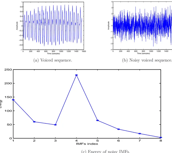
"speech1" and "speech2" corrupted by the factory noise. The results are reported for EMD-ACWA, ACWA ﬁlter and wavelet(db4) . . . . 61 III.1 Frames classiﬁcation scheme. . . 66 III.2 Voiced sequence, noisy voiced sequence and the energy variations of

their noisy IMFs. . . 69 III.3 Not voiced sequence, noisy not voiced sequence and variations of the

energies of its noisy IMFs. . . 70 III.4 Unvoiced sequence, noisy unvoiced sequence and variations of the

(29)

LIST OF FIGURES 9

III.5 The stationarity index of a noisy transient frame. . . 72 III.6 Energy variations of the IMFs of the sub-frames. . . 72 III.7 Original signals /o/, /a/, /e/ and /i/. . . 74 III.8 Noisy versions of signals /o/, /a/, /e/ and /i/ (input SNR=2 dB). . . 74 III.9 Decomposition of noisy signal /o/ into IMFs (input SNR= 2dB) . . . 75 III.10Variations of CMSE (energy) values versus the number of IMFs for

the four noisy signals. . . 75 III.11Enhanced signals obtained by the proposed method, Wavelet (db4),

ACWA ﬁlter and EMD-ACWA (input SNR=2 dB). . . 77 III.12Variations of output SNR versus input SNR for signals /o/, /a/, /e/

and /i/. The results are average over 100 noise realizations. The reported results correspond to the proposed method, Wavelet(db4), ACWA ﬁlter and the EMD-ACWA. . . 78 III.13Variations of PESQ values versus input SNR for the signals /o/, /a/,

/e/ and /i/. The results are average over 100 noise realizations. The reported results correspond to the proposed method, wavelet(db4), ACWA ﬁlter and the EMD-ACWA. . . 79 III.14Original signals "speech1", "speech2", "speech3" and "speech4". . . 80 III.15Noisy version of signals "speech1", "speech2", "speech3" and "speech4"

(input SNR = 2 dB). . . 80 III.16Denoising of noisy signals "speech1", "speech2", "speech3" and

"speech4" ( input SNR=2 dB) by the proposed method, Wavelet (db4), ACWA ﬁlter and EMD-ACWA. . . 81 III.17Final SNR values obtained from diﬀerent initial noise levels of signals

"speech1", "speech2", "speech3" and "speech4". The results averages over 100 Monte Carlo simulations of the additive noise. It is reported for the proposed method, wavelet(db4), ACWA ﬁlter and the EMD-ACWA. . . 82 III.18PESQ values obtained from diﬀerent initial noise levels of signals

"speech1", "speech2","speech3" and "speech4". It is reported for pro-posed method, Wavelet(db4), ACWA ﬁlter and the EMD-ACWA. . . 83 IV.1 Original IMF and its estimated version by spline interpolation. . . 88

(30)

LIST OF FIGURES 10

IV.2 IMF mean envelope oﬀset . . . 89 IV.3 IA, IP and IF of an IMF. . . 90 IV.4 Encoding scheme. . . 91 IV.5 Encoding scheme. . . 93 IV.6 Decomposition of an audio frame by EMD. . . 95 IV.7 Partial autocorrelation coeﬃcient for IF of IMF generated by audio

frame (ﬁgure IV.6). . . 96 V.1 IMFextrema encoder architecture in context of audio signals. . . 101

V.2 LEC variation for an audio frame. . . 102 V.3 Example of segmentation for an audio frame. . . 102 V.4 Quantization scheme. . . 104 V.5 Original audio signals (gspi, harp, quar, song, trpt and violin). . . 105 VI.1 Decomposition of an audio frame into IMFs. . . 113 VI.2 Data structure {mi}. . . 113

VI.3 Watermark embedding. . . 113 VI.4 Decomposition of the watermarked audio frame by EMD. . . 114 VI.5 Watermark extraction. . . 115 VI.6 Illustration of the last IMF of an audio frame before and after

water-marking. . . 115 VI.7 Binary watermark. . . 119 VI.8 A portion of the pop audio signal and its watermarked version. . . 119 VI.9 PF P E versus synchronization code length. . . 123

(31)

List of Tables

1 Résultats de la compression par EMD, MP3 et par ondelette. . . xv 2 TEB et NC de la marque extractée pour le signal audio "Rock" par

l’approche proposée. . . xviii 3 Performance des algorithmes de tatouage, trier par débits. . . xviii I.1 Matrix of orthogonality of the signal (Eq. I.7) . . . 32 II.1 Variations of the output SNR and of the PESQ over the input SNR

for the MMSE and ACWA ﬁlters. . . 55 III.1 C and js values of each signal . . . 76

III.2 Denoising results, based on the output SNR, of four noisy voiced different signals (input SNR=2 dB) . . . 76 IV.1 Offset values of IMFs extracted from an audio frame. . . 88 IV.2 Order of AR model for IF of IMFs (figure IV.7). . . 96 V.1 Compression results of audio signals (gspi, harp, quar, song, trpt and

violin) by IMFextrema, IA − IP , AAC, MP3 and the wavelet. . . 106

V.2 Compression results of audio signals (gspi, harp, quar, song, trpt and violin) by IMFenvelope, IA − IF , AAC, MP3 and wavelet methods. . 107

VI.1 SNR and ODG between original and watermarked audio. . . 120 VI.2 BER and NC of extracted watermark for pop audio signal by proposed

approach. . . 121 VI.3 BER and NC of extracted watermark for diﬀerent audio signals

(32)

LIST OF TABLES 12

VI.4 BER and NC of extracted watermark for diﬀerent audio signals (Clas-sical, Jazz, Rock) by proposed approach. . . 123 B.1 Impairment grade. . . 142

(33)

(34)

ABBREVIATIONS 14

Abbreviations

AAC Advanced Audio Coding

ACWA Adaptive Center Weighted Average AM Amplitude Modulation

AR Auto Regressive BER Bit Error Rate BR Bit Rate

CMSE Consecutive Mean Square Error DCT Discrete Cosine Transform DFT Discrete Fourier Transform EMD Empirical Mode Decomposition FFT Fast Fourier Transform

FM Frequency Modulation FNE False Negative Error FPE False Positive Error FT Fourier Transform

HHT Hilbert-Huang Transform IA Instantaneous Amplitude IF Instantaneous Frequency

IFPI International Federation of the Photographic Industry IP Instantaneous Phase

IMF Intrinsic Mode Function LEC Local Entropic Criterion MAE Mean Absolute Error MSE Mean Square Error

NC Normalized Cross-correlation NMR Noise to Mask Ratio

ODG Objective Diﬀerence Grade

PESQ Perceptual Evaluation of Speech Quality QIM Quantization Index Modulation

PDE Partial Diﬀerential Equation SC Synchronized Code

(35)

Introduction

Signals can be derived from diﬀerent sources, but most of them, arising from physical phenomena, are non-stationary. Locally, these signals can be regarded as stationary and thus decomposed as a superposition of sine waves, the frequency of which evolves over time. Among non-stationary signals, we can distinguish speech and audio signals. Conventional tools such as Fourier Transform (FT) and Discrete Cosine Transform (DCT) are unsuitable to analyze non stationary signals. In fact, when the signal spectrum is time varying, such as for music, speech and biomedical signals, time-frequency analysis approach is more relevant. The results of a time-frequency analysis depend on the choice of the time-frequency decomposition tool used, such as Short-Time Fourier Transform (STFT), Wigner distribution or Wavelet Transform (WT).

In several scenarios, it is preferable to take advantage of multi-resolution character-istics of WT. A limit of the wavelet approach is that first, the basis function must be specified and, second a specific basis function may not be able to catch all the non stationarity of the analyzed signal. To overcome this drawback time-frequency atomic signal decomposition can be used [31],[56]. As for wavelet packets, if the dictionary is very large and rich enough with a large collection of atomic waveforms which are located on a much finer grid in time-frequency space than wavelet and cosine packet tables, then it should be possible to faithfully represent a wide range of real signals. Furthermore, the ideal is to find an adaptive decomposition of the signal, so that it does not require a priori information about the signal time varying characteristics.

Recently, a new data-driven technique, referred to as Empirical Mode Decom-position (EMD) has been introduced by Huang et al. [34] for analyzing data resulting from non-stationary and nonlinear processes. EMD has received much attention in terms of applications [3],[7]-[9] interpretation [33]-[35], and improve-ment [16],[84]. Major advantage of EMD is that the basis function is derived from

(36)

INTRODUCTION 16

the signal itself. Hence, the analysis is adaptive, in contrast to the traditional methods where the basis functions are fixed. The EMD is based on the sequential extraction of energy associated with various intrinsic time scales of the signal, called Intrinsic Mode Functions (IMFs), starting from finer temporal scales (high frequency IMFs) to coarser ones (low frequency IMFs). The superposition of the extracted IMFs matches the signal very well and therefore ensures completeness [34]. Characteristics of EMD and its effectiveness as a decomposing tool, have been addressed by different research. Indeed, an improvement in terms of signal decomposition has been shown in [68],[69]. The combination of EMD with Hilbert transform demonstrated the interest of EMD as a tool to investigate time-frequency domain representations [6],[11]. In [21] it has been shown that, provided some hypothesis, the extraction of IMF is reduced to the resolution of partial differential equation (Heat equation). Further, EMD has demonstrated its usefulness and effectiveness in many applications such as biomedical signals filtering and sonar target tracking [6],[11].

Main motivation of this thesis is to investigate the potential of EMD as an analyzing method for both speech and audio signals. More particularly, we address the problems of denoising, coding and watermarking. Also the goal of this work is to explore the limit of self-adaptive nature of the EMD process as signal analyzing tool in speech and audio processing.

Outline of the thesis

The dissertation is organized chapter by chapter as follows

chapter I is devoted to a presentation of the Huang transform, known as EMD.

In particular, interest is focused on the relevant parameters which have inﬂuences on extracted IMFs, such as interpolation and sampling [34],[69]. The capability of EMD for separation of components is also studied and illustrated.

In the ﬁrst part of the thesis, we are interested in techniques of noise reduction (ﬁltering and denoising). Particularly in the case of additive white Gaussian noise,

(37)

INTRODUCTION 17

different approaches have been proposed [72],[75]. When the noise distribution can be estimated accurately, then filtering yields acceptable results. However, these methods are not so effective when the noise level is difficult to estimate. Linear methods based on Wiener filtering [67] are sometimes preferred because linear fil-ters are easy to implement and design. However, linear filtering methods are not so effective when signals contain sharp edges and impulses of short duration. Further-more, real signals are often non-stationary. In order to overcome these shortcom-ings, nonlinear methods have been proposed and especially those based on wavelets thresholding [22],[23]. The idea of wavelet thresholding relies on the assumption that signal magnitudes dominate the magnitudes of the noise in a wavelet repre-sentation, so that wavelet coefficients can be set to zero if their magnitudes are less than a pre-determined threshold [22]. Using the same strategy as in wavelets thresholding approach, we propose in this thesis new techniques of speech denoising based on EMD. Our contribution related to these techniques are organized into two chapters.

In Chapter II, different denoising strategies based on EMD that address both additive white and colored noise are presented. In fact, it has been shown in [7]-[9], that EMD can be used for signal denoising. The proposed denoising method reconstructs the signal from all the IMFs previously filtered or thresholded as in wavelet analysis [7]-[9]. In this chapter, firstly two new denoising strategies for white noise context are presented. The first strategy combines EMD and Minimum Mean Squared Error (MMSE) filter [75], and the second one associates EMD with hard shrinkage [7]-[9]. The two methods, effective for a large class of signals, are applied to speech signals corrupted with different white noise levels.

The third denoising technique, called EMD-ACWA, consists in filtering IMFs by Adaptive Center Weighted Average (ACWA) filter [52], which exploits some local statistics of the signal. This technique is efficient both in the context of white noise and colored one. The use of ACWA filter is motivated by two important reasons. First, it operates in the time domain as the EMD. So, there is no need to use of FT as in the case of the MMSE filter [75]. Second, the ACWA filter operates regardless of the nature of the signal and noise. In particular, the assumptions of signal stationarity and white noise are not required.

Chapter III deals with a new noise reduction technique dedicated to speech

(38)

INTRODUCTION 18

the characteristics of speech signal. The proposed approach takes into account the class of the processed speech frame (voiced/unvoiced and transient). Indeed, in the IMF filtering step the number of denoised IMFs depends on whether the noisy frame is voiced or unvoiced. An energy criterion detects voiced frames while the stationarity index [51] is used to distinguish between unvoiced and transient frames . The second part of the thesis is devoted to audio coding. The coding process is a central topic in the fields of audio and image processing [39],[82] and particularly in audio domain where different strategies have been proposed [40],[64]. When applications are not limited by low bit rate constraints, coding usually leads to acceptable results. However, in many applications such as digital audio broadcasting or multimedia, low bit rate and high fidelity are required. In order to reduce the bit rate, sub-band coding [10],[78] and transform coding approaches [20],[74] have been used to design efficient coding algorithms. These methods use basically a subband decomposition of the signal followed by perceptual encoding of significant coefficients at each subband which appeals to the following principle: do not code

what the ear can’t listen. Applying this principle enables good results at low bit

rate. Unfortunately, using a decomposition strategy based on the representation on a fixed basis prevents the decomposition from being parsimonious for any kind of audio signal. Indeed, even if a decomposition tool is well suited for a large class of audio signals, in the sense that it yields compact descriptions with only a few significant terms, there are audio signals for which the basis under consideration performs poorly [20]. The EMD can be seen as a type of subband decomposition whose subbands are able to automatically separate the different components of a signal. Each IMF replaces the signal details, at a certain scale or frequency band. Thanks to IMF properties, the EMD seems to be a very interesting decomposition tool to use for a low bit rate audio coding. The presentation of our contribution to audio coding is organized in two chapters.

In chapter IV, a new signal coding based on EMD is introduced. The ﬁrst step consists in encoding the IMFs extrema, since the IMFs are fully described by their local extrema [34]. To further reduce the bit rate, only one of the IMFs envelops is encoded. This is motivated by the quasi-symmetrical property of the IMF. In a second step, a waveform coding approach based on EMD in association with Hilbert transform is presented. Based on the Hilbert and Huang transforms,

(39)

INTRODUCTION 19

we can calculate the Instantaneous Amplitude (IA), Instantaneous Phase (IP) and the Instantaneous Frequency (IF) for IMFs. The idea is then to encode the IA and IF by linear prediction, while the IP is encoded by a scalar quantization.

Chapter V is devoted to apply the proposed coding approaches, described in

the previous chapter to audio signals. We show that it is interesting to introduce a psychoacoustic model, in extrema thresholding and bit allocation; and detector for transient sequence in these approaches. The performance of the proposed methods are analyzed and compared to the MPEG1 layer3, known as MP3, to AAC codecs and to the wavelet based compression.

Watermarking is as a solution to control unapproved copying and redistribution of multimedia data, where many bit streams can be transmitted by taking the audio signal as a transmission medium. Various constraints must be considered in the watermarking process such as inaudibility of the watermarked signal, higher transmission bit rate and robustness against distortions. The detection of the in-serted message is the subject of several research [2],[79] where several watermarking techniques have been proposed [13],[41]. The watermarking approach of Malvar [50] is among of the recent algorithms in the context of audio signals. This approach has shown good robustness to a wide variety of attacks but it imposes a very limited transmission bit rate. So, to increase the bit rate, many watermarking algorithms based on the wavelet has been presented [41],[86]. A limit of the wavelet approach is that the basis functions are ﬁxed, and thus may not be eﬀective for all real signals. The IMFs are fully described by their local extrema [34], thus, they can be constructed from only their extrema [47]. The superposition of extracted IMFs matches the signal very well and therefore ensures completeness [34]. Based on these interesting proprieties, we considered a watermarking scheme based on EMD. The proposed watermarking approach is the subject of chapter VI.

Chapter VI introduces a new audio watermarking approach, based on EMD,

dedicated to control unapproved copying. The watermark and the synchronization codes are embedded into the extrema of the last IMF, a low frequency mode stable under diﬀerent attacks and preserving an audio perceptual quality of the host signal. Relying on exhaustive simulations, we show the robustness of the hidden watermark data to additive noise, low-pass ﬁltering, MP3 compression, re-quantization and denoising. The reported results are compared to watermarking

(40)

INTRODUCTION 20

schemes reported recently.

Finally, the conclusion will review all the work done and presents several sug-gestions and extensions to improve and optimize the contributions of this work.

Main contributions of the thesis

In the following we list the main contributions of the dissertation

• Introduction of a new noise reduction scheme operating in adaptive way. Differ-ent strategies of filtering and denoising of audio signals are developed. Improve-ment in terms of output SNR (Signal to Noise Ratio) and PESQ (Perceptual Evaluation Speech Quality) are obtained compared to MMSE filter and wavelet approach.

• Introduction of a new signal coding framework based on the extrema of IMFs. Diﬀerent coding strategies are presented. No assumptions concerning the lin-earity or the stationary are made about the signal to be coded. The new scheme can be extended to encode any signal and from any source. Improvement in terms of BR (Bit Rate), ODG (Objective Diﬀerence Grade) and NMR (Noise to Mask Ratio) are obtained compared to MP3 and AAC codecs, and wavelet based compression.

• Introduction of a new adaptive watermarking scheme based on the EMD. Wa-termark is embedded in very low frequency mode (last IMF), thus achieving good performance against various attacks. Data bits of the synchronized wa-termark are embedded in the extrema of the last IMF of the audio signal based on quantization index modulation. Extensive simulations over diﬀerent audio signals indicate that the proposed watermarking scheme has greater robust-ness against common attacks than nine recently proposed algorithms. The new scheme has higher payload and better performance against MP3 compression compared to these earlier audio watermarking methods.

(41)

INTRODUCTION 21

List of publications

Denoising

• K. Khaldi, A.O. Boudraa, A. Bouchikhi, and M. Turki, "Speech Enhancement via EMD", EURASIP Journal Advances in Signal Processing, vol. 2008, Article ID 873204, 8 pages, 2008.

• K. Khaldi, M. Turki and A.O. Boudraa, "Voiced speech enhancement based on adaptive ﬁltering of selected Intrinsic Mode Functions", Advances in Adaptive Data Analysis (AADA), vol. 2, n°. 1, pp. 65-80, 2010.

• K. Khaldi, A.O. Boudraa, A. Bouchikhi, M. Turki and E. Diop, "Speech signal noise reduction by EMD", IEEE International Symposium on Communications, Control and Signal Processing (ISCCSP), march 2008, Malta.

• K. Khaldi, A. Adib et M. Turki, "Amélioration des techniques de séparation de sources par débruitage via EMD", Colloque Africain sur la Recherche en Informatique et en Mathématiques Appliquées (CARI), octobre 2008, Rabat, Maroc.

• K. Khaldi, M. Turki and A.O. Boudraa "A new EMD denoising approach dedicated to voiced speech signals", IEEE Signals, Circuits and Systems (SCS), november 2008, Hammamet, Tunisia.

• K. Khaldi, M. Turki and A.O. Boudraa "Speech enhancement by adaptive weighted average ﬁltering in the EMD framework", IEEE SCS, november 2008, Hammamet, Tunisia.

• K. Khaldi, M. Turki and A.O. Boudraa, "Speech denoising using modal de-composition and local statistics", Digital Signal Processing (submitted).

Coding

• K. Khaldi, A.O. Boudraa, M. Turki, Th. Chonavel and I. Samaali, "Audio encoding based on the Empirical Mode Decomposition", IEEE European Signal Processing Conference (EUSIPCO), august 2009, Glasgow, Scotland.

(42)

INTRODUCTION 22

• K. Khaldi, A.O. Boudraa, M. Turki et Th. Chonavel, "Codage audio per-ceptuel à bas débit par Décomposition en Modes Empiriques (EMD)", Col-loque Groupe de Recherche et d’Etudes du Traitement du Signal et des Images (GRETSI), septembre 2009, Dijon, France.

• K. Khaldi, A.O. Boudraa, B. Torrésani, Th. Chonavel and M. Turki, "Au-dio encoding using Huang and Hilbert transforms", IEEE ISCCSP,march 2010, Limassol, Cyprus.

• K. Khaldi, A.O. Boudraa, Th. Chonavel, and M. Turki "Empirical Mode Com-pression (EMC) of audio signals", Signal Processing Journal (First Revision). • K. Khaldi, A.O. Boudraa, B. Torrésani, M. Turki and Th. Chonavel,

"HHT-Based Audio Coding", International Journal of Wavelets, Multiresolution and Information Processing (submitted).

Watermarking

• K. Khaldi and A.O. Boudraa, "Audio watermarking via EMD", IEEE Trans-actions on Audio, Speech and Language Processing (submitted).

(43)

(44)

CHAPTER

I

Huang transform

T

his chapter presents the Huang transform, known as Empirical Mode De-composition (EMD), introduced by Huang et al. [34]. The EMD is a data driven method, defined by an algorithm, that enables the adaptive decom-position of a signal into finite sum of components, called Intrinsic Mode Functions (IMFs). The principle of EMD is presented and is illustrated on synthetic signals. Some parameters, such as interpolation and sampling frequency, which influence the results of the decomposition are point out. Finally, some aspects of the EMD considered as a time-frequency description tool are presented and discussed.

(45)

CHAPTER I. HUANG TRANSFORM 25

I.1 Introduction

In this chapter, we introduce the Huang transform known as Empirical Mode De-composition (EMD). The EMD is introduced by Huang et al, to overcome the limi-tations of Fourier based methods when applied to non-stationary signals. The EMD decomposes adaptively a signal into a sum of oscillating components. Unlike the Fourier Transform (FT) or Wavelet Transform (FT), the EMD is a data driven de-composition technique. It has been introduced for analyzing data deriving from non-stationary and nonlinear processes. The major advantage of the EMD is that the basis functions are derived from the signal itself. Hence, the analysis is adap-tive in contrast to the traditional methods where the basis functions are ﬁxed. The EMD is based on the sequential extraction of energy associated with various intrinsic time scales of the signal or oscillating components, called Intrinsic Mode Functions (IMFs), starting from ﬁner temporal scales (high frequency IMFs) to coarser ones (low frequency IMFs). The total sum of the IMFs matches the signal very well and therefore ensures completeness [34].

I.1.1 Principle of EMD

The EMD is an algorithmic signal decomposition method. It is based on the principle of decomposing a signal into the sum of a high frequency component (fast oscillation) and a low frequency component (trend). This principle is illustrated by equation ( I.1),

x(t) = d(t) + m(t), (I.1)

where t denotes the discrete time, x(t) is the signal to decompose, d(t) is the fast oscillation and m(t) is the signal trend. Similarly, the signal trend can also be decomposed into two terms,

m(t) = d1(t) + m1(t), (I.2)

where d1(t) is the high frequency component of m(t), and m1(t) is its low frequency

component.

To extract the mode of a signal x(t), the following principle is considered: • identify all extrema of x(t).

(46)

CHAPTER I. HUANG TRANSFORM 26

emin(t) (resp emax(t)).

• compute the average m(t) = (emin(t)+ emax(t))/2.

• extract the detail d(t) = x(t) − m(t).

The signal d(t) is considered as IMF after a number of iterations needed to satisfy a given stop criterion. By iterating this principle to the obtained trends, we get a signal decomposition described as follows:

x(t) =

C

X

j=1

IMFj(t) + rC(t), C ∈ N∗ (I.3)

where IMFj is the jth order IMF. IMFj contains higher frequency oscillations than

the IMFj+1. The signal rc(t) is called the residual, it is the lower frequency

com-ponent of signal x(t). According to Eq. I.3 and assuming that C is ﬁnite, we can construct linearly the original signal without loss of any information [34].

By deﬁnition, a component is considered as a true IMF if it satisﬁes the following criteria [34]:

1. the number of its extrema and the number of its zero crossings may diﬀer by no more than one.

2. the average value of the envelope deﬁned by the local maxima and the envelope deﬁned by the local minima, is zero.

I.1.2 EMD algorithm

The principle of IMFs extraction is ensured by the sifting process, which is implemented by the following generic algorithm.

Notations:

ǫ: predetermined threshold, that is used to specify the loop exit condition. j: IMF index.

i: index of current iteration in the loop for extracting an IMF. T: length of the decomposed signal: x= x(t)t=1...T.