Science Arts & Métiers (SAM)
is an open access repository that collects the work of Arts et Métiers Institute of Technology researchers and makes it freely available over the web where possible.
This is an author-deposited version published in: https://sam.ensam.eu
Handle ID: .http://hdl.handle.net/10985/17239
To cite this version :
Tristan RÉGNIER, Bertrand MARCON, José OUTEIRO, Guillaume FROMENTIN, Alain
D’ACUNTO, Arnaud CROLET - Investigations on exit burr formation mechanisms based on digital image correlation and numerical modelling - Machining Science and Technology - Vol. 23, n°6, p.925-950 - 2019
Any correspondence concerning this service should be sent to the repository Administrator : [email protected]
1
INVESTIGATIONS ON EXIT BURR FORMATION MECHANISMS BASED ON DIGITAL IMAGE CORRELATION AND NUMERICAL MODELLING
Tristan Régnier*a, c, Bertrand Marcona, José Outeiroa, Guillaume Fromentina, Alain D’Acuntob, Arnaud Croletc
aLaBoMaP – Arts et Métiers Paristech Cluny, Rue porte de Paris, 71250 Cluny,
France
[email protected], [email protected], [email protected], [email protected]
bLEM3 – Arts et Métiers Paristech Metz,7 rue Félix Savart, 57073 Metz, France
cLINAMAR – MONTUPET, 3 rue de Nogent, 60290 Laigneville, France
[email protected], [email protected]
*Corresponding author: Tristan Régnier E-mail: [email protected]
Address: Arts et Métiers, Campus of Cluny, Rue porte de Paris, 71250 Cluny, France
Abstract
Requirements on burr height and burr amount on machined parts are getting stricter. This leads to method development from manufacturing companies to predict burr distribution and its size along part edges. A deeper understanding of burr formation mechanisms will assist to more accurate model development.
This study aims to analyze the exit burr formation, which is formed during orthogonal cutting of a brittle cast aluminum alloy. A customized Digital Image Correlation (DIC) system with
2
the help of a high-speed camera was used to measure the displacements fields. It calculates strain fields during burr initiation and development in orthogonal cutting of T7 heat-treated cast Aluminum alloy ENAC-AlSi7Mg0.3 as well. Those results are then qualitatively compared with a numerical model of the burr with chamfer formation developed and simulated using a Finite Element Method (FEM), to ensure a good correspondence between experiments and simulation. This model is used to complete the DIC study of burr with chamfer formation mechanisms during crack propagation leading to chamfer formation. The analysis of numerically obtained stress triaxiality fields and of DIC observations from experiments are compared to the assumptions made from analytical models. Finally, necessary improvements of an existing burr formation analytical model are proposed.
Keywords
Burr formation mechanisms; Digital Image Correlation (DIC); Aluminum alloy; Numerical simulation; Analytical modeling
Introduction
A burr is defined by the standard ISO 13715 (2017), as a “rough remainder of material outside the ideal geometrical shape of an external edge, residue of machining or of a forming process”. As explained by Aurich et al. (2009), nowadays, more and more manufacturing companies are trying to reduce burr formation during machining to avoid or to reduce the use of additional burr-removal techniques. Simultaneously, requirements on burrs remaining on a finished part are getting stricter.
Gillespie and Blotter (1976) pointed out the difference between four main burr formation mechanisms in several machining operations:
3
- the Poisson burr, resulting from a plastic deformation of the workpiece around the tool;
- the roll-over burr, resulting from the displacement of the uncut material along the exit edge of the workpiece;
- the tear burr, produced during the separation between the chip and the workpiece; - the cut-off burr specific burr occurring during a cut-off operation.
Iwata et al. (1982) found three burr morphologies that can be generated depending on the effective strain level during exit burr formation using orthogonal cutting, and they identified a zone with negative shear when the burr initiated. According to Iwata et al. (1982), “positive burr” occurs when the effective strain is low enough to avoid fracture along the negative shear zone. If fracture occurs along the negative shear zone, a “negative burr” is formed. Sometimes, fracture occurs along this last zone but not completely (i.e., the obtained burr was referred to as “remained part of chip”). In a recent study, Régnier et al. (2018a) analyzed exit burr formation during orthogonal cutting of the cast aluminum alloy
ENAC-AlSi7Mg0,3+0,5Cu. They showed that the burr morphology varied along the exit edge of the workpiece, namely, both negative and positive burrs (respectively designated as burrs with/ without chamfer) were produced simultaneously. Since the cutting edges and sample
geometries were constant along the width of cut, this phenomenon was thought to be caused by microstructural effects. Furthermore, the amount of each type of burr along the exit edge was controlled by the uncut chip thickness. New burr size parameters were also proposed to define more precisely burr morphologies and to improve their characterization.
As far as analytical modelling of burr formation is concerned, few analytical models have been developed. Ko and Dornfeld (1991) divided burr formation into three steps: burr initiation, burr development and final burr formation. Burr initiation corresponded to the onset of the negative shear zone suggested by Iwata et al. (1982). It was characterized by a
4
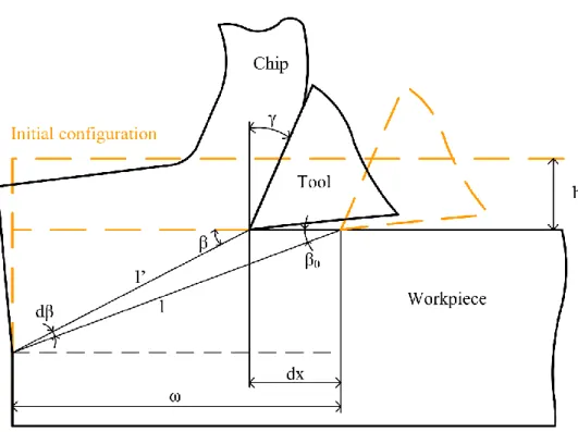
tool distance at initiation (ω) and an initial negative shear angle (β0) (Figure 1). During burr
development, the negative shear zone was assumed to rotate around a pivoting point called burr root.
The authors assumed that burr formation was the result of two mechanisms: shear and bending. To determine the values of β0 and ω, the minimum energy principle and the
hypothesis of energy conservation between chip and burr formation were applied
respectively. However, the model did not correspond to experimental results. It was found that the assumption made on work conservation was not appropriate and the negative shear angle varied from one material to another. To compare the model with experimental results, actual experimental observations on tool distance at initiation () were used by the authors instead of the calculated ones. Later, Ko and Dornfeld (1996a) and Ko and Dornfeld (1996b) applied McClintock’s fracture criterion to model burr with chamfer formation and determine which burr was formed with respect to the cutting conditions. The authors then adapted this model to oblique cutting.
A similar model was developed by Chern and Dornfeld (1996). The authors assumed that the mechanisms of burr formation are generated mainly from shear and bending. The tool
distance at initiation was obtained geometrically and the negative shear angle was again obtained using the principle of minimum energy. Both parameters are calculated analytically based on other parameters such as primary shear angle and uncut chip thickness. The shear angle was assumed to be dependent on the tool rake angle only but it may lead to inaccurate results.
To improve these two analytical models, Hashimura et al. (1999b) proposed a new description of burr formation mechanisms, from its initiation until the end of the cut. As shown in Figure 2, this description was based on SEM and in-situ observations using an optical microscope during orthogonal cutting of copper and AlCu4Mg1 aluminum alloy. A
5
distinction between initiation and development was made and was strain distribution
dependent. Burr development occurred when both strained zones located around the tool and around the exit surface of the workpiece intersect each other. This phenomenon corresponds to the “initiation” defined by Chern and Dornfeld (1996). However, the cutting speed was very low (0.000025 m.s-1), so the model will have to be validated for more realistic cutting speeds (i.e. several m.s-1). Finally, the authors explained that the burr morphology (with or
without chamfer) was dependent on the ductility of the workpiece material, and strain distribution was not compared between cutting conditions exhibiting burr with and without chamfer. In truth, both burrs can be formed depending on the tool rake angle and uncut chip thickness, as shown by Iwata et al. (1982) and later by Régnier et al. (2018a).
Park and Dornfeld (1999) carried out numerous numerical analyses of burr formation in orthogonal cutting of 304L stainless steel, using the Finite Element Method (FEM) software ABAQUS/Explicit. They modelled burr without chamfer formation. To model material separation during steady-state cutting, they also introduced a ductile failure criterion. The model predictions showed good correspondence with the experimental results, in terms of morphology. Using the implicit FEM software DEFORM 2D, Regel et al. (2009) performed numerical simulations focused on burr with chamfer in orthogonal cutting of C45E steel. After comparing the influence of several fracture models on burr shape, they selected the Cockroft and Latham fracture model to simulate the crack propagation. They then propose a novel method to predict the tool position at crack initiation, analyzing the value of the “hydrostatic bowl”, introduced by Leopold et al. (2005). The hydrostatic bowl is a zone located between the cutting edge and the burr root, where highly negative hydrostatic pressure occurs, in other words, where high mean stress occurs. This last method appears to provide better prediction than the current fracture criteria.
6
understand fully the burr formation and development. Digital Image Correlation (DIC) is a very promising measurement technique which registers several pictures of an object- exhibiting modifications (e.g. structural), taken at several time intervals, to determine
displacement fields at a subpixel resolution and at a high accuracy, with respect to a reference image. The Region Of Interest (ROI), where displacement fields are calculated, is
decomposed into several Zones Of Interest (ZOI) of few pixels for local approaches (Sutton et al. 2009). The development of high-speed cameras now allows DIC to analyze high dynamic strain fields, such as those occur during machining operations. So far, few studies have used this technique in the case of machining. Pottier et al. (2014) applied DIC in
orthogonal cutting on Ti6Al4V titanium alloy to analyze the state of strain along the adiabatic shear zone. The challenges of applying DIC to chip segmentation was outlined. Baizeau et al. (2015) used DIC to analyze the effect of tool rake angle on displacement fields and cutting forces during orthogonal cutting of a hardened steel.
Up until now, burr formation models were based on observations at low cutting speed and some mechanisms were not fully understood, especially those explaining the transition between the two burr morphologies (with and without chamfer). In the present study, the formation mechanisms of exit burrs in orthogonal cutting are analyzed using DIC applied to high speed camera images. This analysis will also help to determine exit burr initiation characteristics (e.g., β0 and ω) more accurately than using existing burr formation predictive
models. The crack initiation during burr with chamfer generation is too fast to be analyzed correctly using DIC with the present set-up (i.e. the time step between two frames is too high). Due to this limitation, finite element simulation is used to complete the study of burr with chamfer formation. Stress triaxiality distributions during burr formation, which are known as one of the major parameters controlling the fracture of a material, are also determined using this numerical method. Finally, the accuracy of an analytical model
7
developed by Chern and Dornfeld (1996) is compared to the novel approach with the proposed improvements.
Experimental details and parameters of the study 2.1 Experimental set-up and approach
Orthogonal cutting tests are conducted in a 3-axis Computer Numerical Control (CNC) milling machine DMG DMC85V equipped with linear motors. The cutting speed is generated by the X-axis displacement and set at its maximum speed of 120 m.min-1 (Figure 3a). Since a
cutting speed lower than 120 m.min-1 would be too distinct compared to the usual ones (around 400 to 500 m.min-1), this parameter is considered as fixed. However, the applied cutting speed is much higher than the ones used on the previous studies. The sample and its fixation (Figure 3c and Figure 3d) are tightened to a piezoelectric dynamometer Kistler model 9119 AA2 to record cutting forces. To perform DIC analysis, a high-speed CCD camera PHOTRON SA-Z records the burr formation during the end of the cutting test. The frame-rate is set at 30,000 fps, ensuring an image acquisition each 0.033 ms (approximately 66.7 µm travelled by the cutting tool) with an exposure time of 1/400,000 s. To get a high magnification of the burr formation zone (tool exit from the workpiece), a ×10 magnification Mitutoyo objective with extended lens tubes are assembled to the camera. A 1.84 × 1.23 mm2
observation area is obtained from an image of 1024 × 688 square pixel resolution with 8-bit dynamic range (256 gray levels), and a pixel calibration of 1.792 µm.pix-1.
DIC analysis is performed using CorreliQ4 software on the images acquired by the high-speed camera. This software uses a finite element type global approach based on Q4P1 shape functions as described by Hild and Roux (2012).
Due to a considerable amount of experiments, one sample is used to perform several tests. Hence, between each test, a deburring operation is applied using an insert moving in the opposite direction of the experiment insert, as shown in Figure 3b. This method ensures a
8
sample free of burrs at the exit edge of the workpiece before a new test. Each cutting condition is performed three times to analyze the result’s variability.
A laser profilometer Keyence model LJ-V7060 is assembled on the Z-axis spindle after each test to perform in-situ measurement of exit burr topography after machining, using an
optimized protocol detailed by Régnier et al. (2018). 2.2 Cutting conditions and work material
The work material used in this study is a T7 heat treated cast Aluminum alloy ENAC-AlSi7Mg0.3 with 0.5% Cu. Samples are extracted from cast billets by milling. Mechanical properties of different regions of the billets are obtained from several quasi-static tensile tests and listed in Table 1.
The inserts used in the study are all uncoated tungsten carbides grooving inserts from ARNO and modified by an edge sharpening company to obtain the specified geometries. Two different tool rake angles are used (-10° and 10°) to analyze their effect on burr morphology. A small tool inclination angle is applied to the inserts to avoid generation of a lateral burr along the side edge facing the camera. Initially, two cutting edge radii were studied but statistical analysis carried out by Régnier et al. (2018) did not show a major influence of this parameter, in this range of variation. Therefore, only results with a 10 µm cutting edge radius will be considered in this study. Cutting conditions and insert specifications are shown in Table 2. All the tests were conducted under dry cutting conditions.
All the experimental results, in terms of burr geometric criteria, will be used to evaluate the analytical model developed by Chern and Dornfeld (1996). Nevertheless, DIC analysis is performed for relatively high uncut chip thickness, to perform a better analysis of strain and displacement fields. Finally, numerical simulation will be used to have a closer look on burr with chamfer and provide information on stress triaxiality distribution at burr formation. The results of both methods will be compared to the burr formation processes described by
9
Hashimura et al. (1999b) to confirm their observations. A comparison with the model developed by Chern and Dornfeld (1996), is also proposed to point out some elements of their model which could be improved, and how one can improve it.
Burr formation analysis using DIC
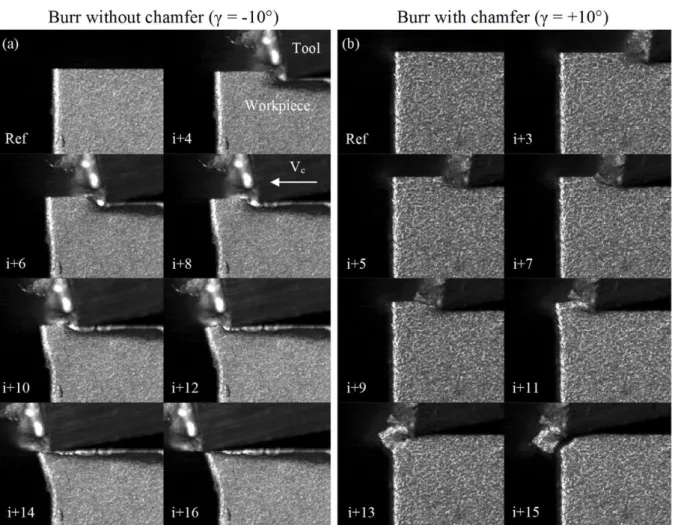
Severe DIC errors can occur when applied to burr formation, due to the high strain and strain-rate genestrain-rated by machining. Sometimes, calculation can’t converge and the ROI (region where computation occurs) is automatically reduced by the software used in the study. To perform an easier and better DIC analysis, the choice of comparing trials conducted at relatively high uncut chip thickness is made. As explained in introduction, the uncut chip thickness and tool rake angle are the main cutting parameters controlling burr morphology. For an identical uncut chip thickness, cutting with a positive rake angle leads to a higher chance of producing a burr with chamfer. On the contrary, burr without chamfer is mainly produced during a cut using a negative rake angle tool. Therefore, the choice is made to vary the rake angle between -10° and +10°, and to keep the uncut chip thickness constant
(0.1 mm). Some selected images showing burr formation with and without chamfer are shown in Figure 4. In this figure, the reference image is noted by ‘Ref’ and the image at burr
initiation is noted by ‘i’.
3.1 DIC parameters and characteristics
ROI definition is critical since it represents the frame where displacements and strain
calculation will be done. If the ROI is too small, some information will be lost. Since the exit edge geometry will change during burr formation, the ROI has to take into account the increase of the considered surface. To do so, ROI are defined as shown in Figure 5a, but an exclusion region is added to avoid calculation where no material exits. A suitable pattern for DIC analysis must be generated over the sample surfaces under observation from the camera, in order to display a maximum number of grey levels. Therefore, each sample used in the
10
study were polished and then shot-peened using glass micro-beads with 50 µm to 100 µm diameters, at 1 bar pressure. Unfortunately, some samples’ side edges are rounded due to polishing, exhibiting to brighter pixels. Figure 5b displays the grey level histogram of the ROI for one of the tested conditions. For the case of negative tool rake angle and high uncut chip thickness, a small lateral burr was formed, despite the tool inclination angle. To avoid computation errors, the ROI applied to those cutting tests was smaller when compared to other cutting conditions.
The ZOI (area of several pixels composing the ROI) size is set to 16 × 16 square pixels based on an a priori analysis estimating the lower ZOI size, which can be chosen based on the ROI grey level distribution, displacement uncertainty and noise sensitivity. Since large
displacements occur during burr formation, 5-pixel coarsening scales are chosen to perform the DIC calculations. A maximum of 200 iterations were used. All the displacement and strain fields are plotted over the reference images.
To obtain the material displacement due to the cutting, the rigid body motion was determined by the Correli Q4 software and was removed from the total displacement field.
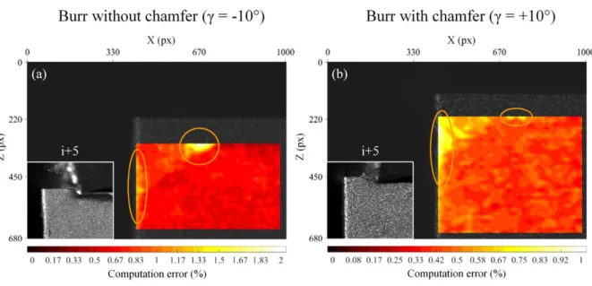
The distribution of the DIC calculation errors should be considered for the analysis of the material displacement fields. Zones with high DIC calculation errors should be excluded from this analysis, which can be due to several factors, including: grey level distribution, lighting, etc. Figure 6 shows typical distributions of DIC calculation errors for both types of burr formation.
This figure shows that the error is maximum around the tool cutting edge. This observation can be explained by some out-of-plane material displacement (chip and lateral burr) formed during cutting. High strain and strain-rate occurring around the cutting edge between two images can also increase residuals error. Some “high” error patterns are observed along the exit edge of the workpiece. Considering that a maximum error of 2% is reasonable and that
11
most of the regions impacted by burr formation exhibit lower error, the results obtained from DIC are considered acceptable.
The terms “burr initiation” and “burr development” are in accordance to the definitions proposed by Hashimura et al. (1999b). The terms introduced by Ko and Dornfeld (1991), “tool distance at initiation” (ω) and “initial negative shear angle” (β0) are modified to
“development distance” and “deformation angle” respectively, to avoid any confusion. The new term “initiation distance” defines the distance between the cutting edge and the exit edge of the workpiece when burr initiates.
3.2 Burr initiation and development
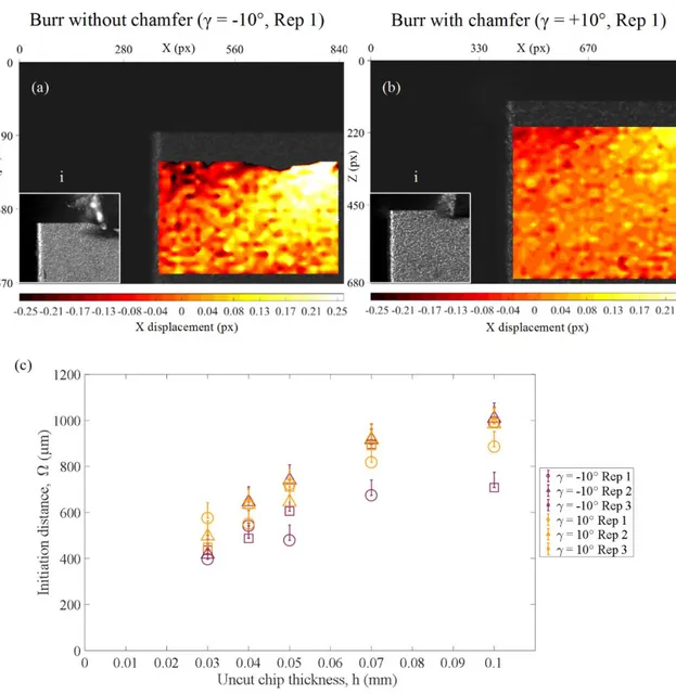
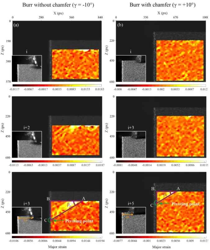
Before analyzing both burr morphologies development, burr initiation is investigated. To identify the initiation distance, the horizontal displacement field evolution is studied. In Figure 7a and Figure 7b, the transition between steady state cutting and burr initiation is established for both cutting conditions analyzed. After determining the image corresponding to burr initiation, the distance between the cutting edge and the exit surface of the workpiece can be measured on the raw images with an uncertainty of approximately 70 µm (distance travelled by the tool between two images). All the measured initiation distances are plotted in Figure 7c. As previously observed by Hashimura et al. (1999b), burr initiation distance tends to increase with respect to the uncut chip thickness.
Strain analysis is conducted starting from the burr initiation image, to identify burr development a. Major strain evolutions from initiation to development are displayed in Figure 8a and Figure 8b. One can discern the growth of the deformation zone from the cutting edge to the pivoting point. Once development distance is established, the burr development characteristics β0 and ω can be measured from the last image, and will be
12
compared in the last section to the results of the predictive model developed by Chern and Dornfeld (1996).
The triangle ABC representing the initial displacement field of the burr initiation is delimited by the cutting edge (A), the exit corner of the workpiece (B), and the forthcoming burr root (C). Although for low uncut chip thickness (h = 0.03 mm and h = 0.04 mm), burr root starting location is quite difficult to identify, for higher uncut chip thickness, the link between them is conspicuous and corresponds to Hashimura et al. (1999b) observations.
3.3 Burr propagation without chamfer (γ = -10°)
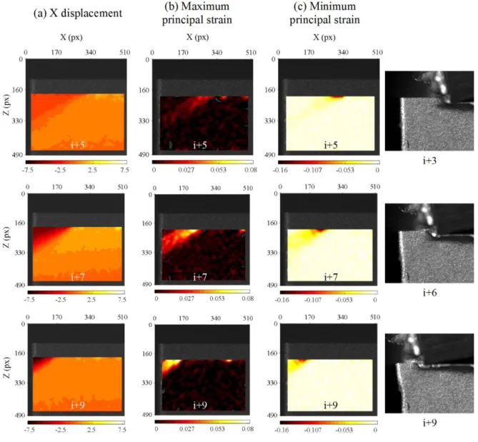
Maximum and minimum principal strain distributions of burr propagation without chamfer are represented in Figure 9b and Figure 9c for three step times. The localized high strain zone seems to follow the cutting edge, while keeping the same orientation. The same happens for the horizontal displacement distribution shown in Figure 9a, i.e. β remains constant during the whole process of burr without chamfer formation. A different assumption was made by Chern and Dornfeld (1996), which considers a rotation of the high localized strain zone during burr propagation (around the pivoting point). In fact, several high localized strain zones with the same orientation are generated during tool displacement. This succession of localized high strain zones seems to pilot the burr root diameter. The strain state evolution and intensity visible in Figure 11a and Figure 11c respectively (observed where the
equivalent strain is significant), confirm this observation. A high compression zone acts as a boundary between the currently deformed area, where pure shear occurs, and the rest of the sample. The presence of such compression state reduces considerably the possibility of a crack initiation. Since no rotation occurs during burr without chamfer formation, the term “pivoting point” is not appropriate and should be renamed “burr root initiation zone”.
13 3.4 Burr propagation with chamfer (γ = +10°)
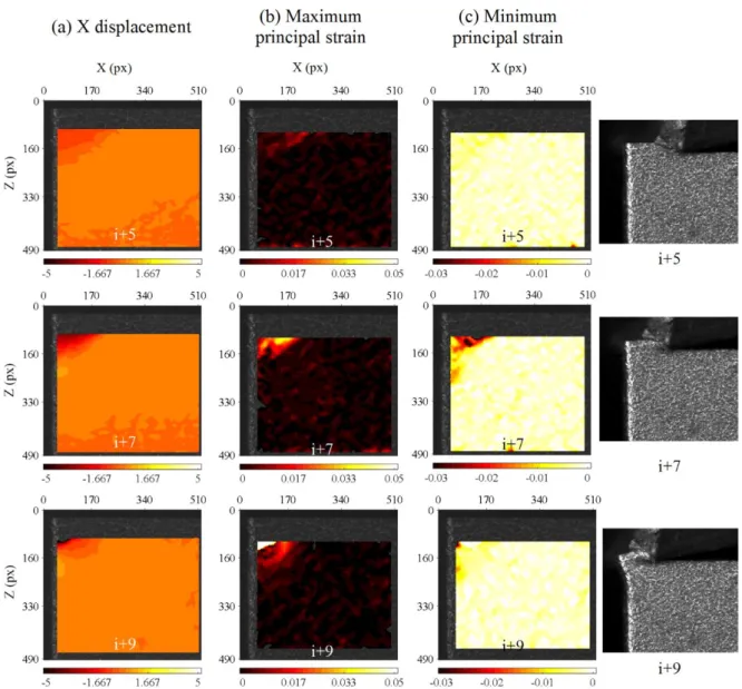
In the case of burr without chamfer, cracks always propagate in the cutting direction. Therefore, material is separated from the workpiece to form the chip (Astakhov 1998). As for the case of burr with chamfer, the direction of crack propagation is deviated from the cutting direction in the instant to form the chamfer. This kind of crack propagation is located within of the ZOI, which makes DIC difficult or even impossible. Nevertheless, the strain distribution right before the changing of crack direction gives useful information to understand the mechanisms of burr formation with chamfer.
The evolution of both maximum and minimum principal strains as well as the horizontal displacement during the burr with chamfer are presented in Figure 10. Between images i+7 and i+9, the maximum principal strain increases while the minimum principal strain around the cutting edge decreases. The strain state evolution resulting from both maximum and minimum principal strains are presented in Figure 11b. This figure shows that between the images i+7 and i+9, the strain state around the cutting edge varies from compression to tension, which is in accordance with fractography observations made by Chern (2006b). Finally, the presence of a high compression area around the burr root, visible in Figure 11d, combined to the previous observation, confirms that the overall strain state is propitious to crack propagation within the ZOI to form the chamfer.
Strain state evolution explains the crack propagation located around the cutting edge. However, residual errors are higher around the cutting edge and around the burr root which tempers that observation. Moreover, the area of analysis is quite limited and useful information to understand the burr with chamfer formation may be lacking. To complement these experimental observations and to complete the analysis, numerical simulation of burr formation with chamfer are performed, as described on the following section.
14 4.1 Burr formation model
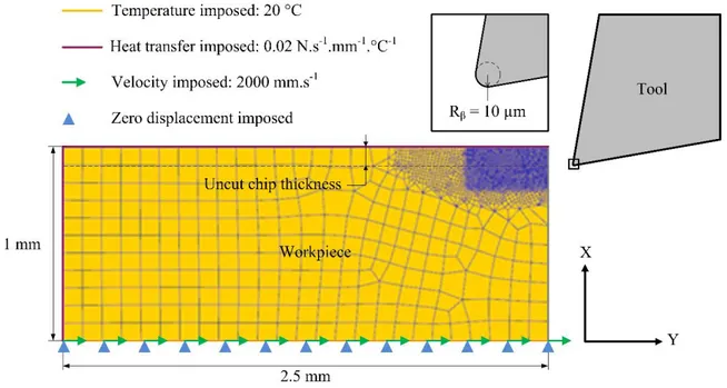
Figure 12 shows the orthogonal cutting model used to analyze burr formation with chamfer under dry cutting conditions. The cutting condition leading to burr with chamfer formation, during DIC analysis, is modelled, (h = 0.1 mm ; γ = +10° ; Vc = 120 m.min-1 ; α = 10° and
rβ = 10 µm).
This model was implemented in the finite element code DEFORM-2D, which uses an implicit algorithm with automatic remeshing. The model was initially discretized in approximately 5,000 elements (to ensure at least 20 elements in the uncut chip thickness) with a minimum element size of 5 µm until burr initiation. At burr initiation, when the stress around the forthcoming burr root increases, the workpiece is remeshed with approximately 10,000 elements, exhibiting a minimum element size of less than 3 µm.
A thermo-mechanical analysis was performed under plane strain conditions. The work-material behavior is considered elasto-viscoplastic. Young modulus and Poisson ratio are given in Table 1, which are used to represent the elastic behavior. To model the plasticity behavior of the work material, stress-strain data from compression tests performed using a Gleeble 3500 machine over cylindrical samples at several strain-rates were used. This data is represented in Figure 13 through flow stress curves fitted from experimental data.
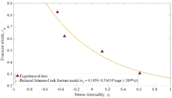
To represent the fracture behavior of the work material, Rice and Tracey (1969) model was used, which is represented by the following equation:
𝐶𝑐𝑟𝑖𝑡 = ∫ 𝑒𝑥𝑝 ( 3 2 𝜎𝑚 𝜎̅) 𝑑𝜀̅ 𝜀̅𝑓 0 (1)
where 𝐶𝑐𝑟𝑖𝑡 is the critical value to be determined, 𝜀̅𝑓 is the strain at fracture, 𝜎𝑚 is the mean
stress, 𝜎̅ is the effective stress, 𝜎𝑚/𝜎 ̅ (or η) represents the stress triaxiality and 𝜀̅ is the equivalent strain. This model is used to describe the fracture behavior of materials which are highly stress state dependent. Figure 14 represents the experimental strains at fracture
15
obtained and the corresponding fitted Johnson-Cook’s fracture criterion. One can easily see here that the increase of stress triaxiality reduces considerably the fracture strain of these materials. The value of 𝐶𝑐𝑟𝑖𝑡 for the ENAC-AlSi7Mg0.3+0.5Cu – T7 aluminum alloy is 0.3854. This value was determined with the combination of both numerical simulations and experimental compression tests on double-notched specimens, following the procedure described by Abushawashi et al. (2013). The compression test simulation provides strain state and stress state during compression. With the aid of DIC, the experiments help to determine the strain at fracture. The evolution of the stress state until the strain at fracture retrieved from the simulation for several pressure angles, is used as input parameters to determine 𝐶𝑐𝑟𝑖𝑡. Element deletion technique was applied to simulate material separation (fracture), when the integral result represented by equation 1 at the finite element is equivalent or exceeds 𝐶𝑐𝑟𝑖𝑡.
The material behavior of the tool was considered rigid, and the corresponding physical properties are taken from DEFORM software database for uncoated tungsten carbide. Tool-chip and tool-workpiece contacts were modelled using a constant shear factor coefficient (m), set to 0.8 based on orthogonal cutting theory (Merchant 1945) and on the overall forces measurements.
The predicted results were compared to the experimental ones concerning the chip
compression ratio (CCR), forces, chamfer height, chamfer depth and burr height, as shows Table 3.
A comparison between the equivalent strain fields measured with DIC and simulated at the beginning of burr development is presented in figure 16. The strain intensity obtained by simulation represents from 50 to 80% of the equivalent strain calculated by DIC. This difference is due to errors associated to both experimental determination of strains by DIC and FEM analysis. This aspect must be improved to carry out some quantitative analysis but it is considered acceptable to analyze the overall behavior of the material during burr formation.
16
Even though the predicted CCR and forces are lower than the experimental ones, the predicted burr characteristics and plastic strain are close to experimental ones. Thereby, an analysis of burr formation with chamfer is carried out using this model.
4.2 FEA of burr formation with chamfer
To improve the understanding of the mechanisms leading to burr formation with chamfer, the evolution of equivalent plastic strain and stress triaxiality distributions during burr initiation and propagation are investigated. These distributions are represented in Figure 16a and b for the cutting conditions mentioned on the previous section.
Figure 16a shows that the equivalent plastic strain distribution during burr initiation and propagation is in good correspondence with Hashimura et al. (1999b) observations and the experimental results presented in previous sections: during burr initiation, strain increases around both the forthcoming burr root and the cutting edge, then, both strain zones intersect each other and burr development starts. Moreover, the stress state analysis provides information about chamfer generation mechanism: stress triaxiality increases from burr initiation to burr propagation. A positive stress triaxiality zone (an indicator of tensile stress state), localized underneath the cutting edge, expands until it reaches the cutting edge. Crack initiation begins and it propagates until the burr with chamfer is fully formed.
Comparison between experimental observations and analytical modelling
As explained in introduction, an analytical model of burr height prediction developed by Chern and Dornfeld (1996) is applied, and its validity in relation to the work material used in this study is discussed. Several features are compared:
- Shear angle
- Burr propagation distance - Deformation angle, β0
17
- Main burr morphology along the exit edge (with or without chamfer) - Burr height or chamfer height depending on the main burr morphology
Firstly, the aim of this comparison is to discuss about the accuracy of the predictive model for ENAC-AlSi7Mg0,3+0,5Cu alloy cutting. Next, the comparison analyzes predicted features if they are over or under estimated and subsequently a few proposals are suggested to improve the model.
Burr height and chamfer height obtained from the model and the experiment are represented in Figure 17 in function of the uncut chip thickness. Since almost no burr with chamfer is produced with the negative tool rake angle and the same for burr without chamfer and
positive tool rake angle and the same goes to burr without chamfer height and chamfer height are plotted in function of tool negative and positive rake angles respectively. It is observed that chamfer height prediction is quite accurate but burr height prediction is slightly overestimated.
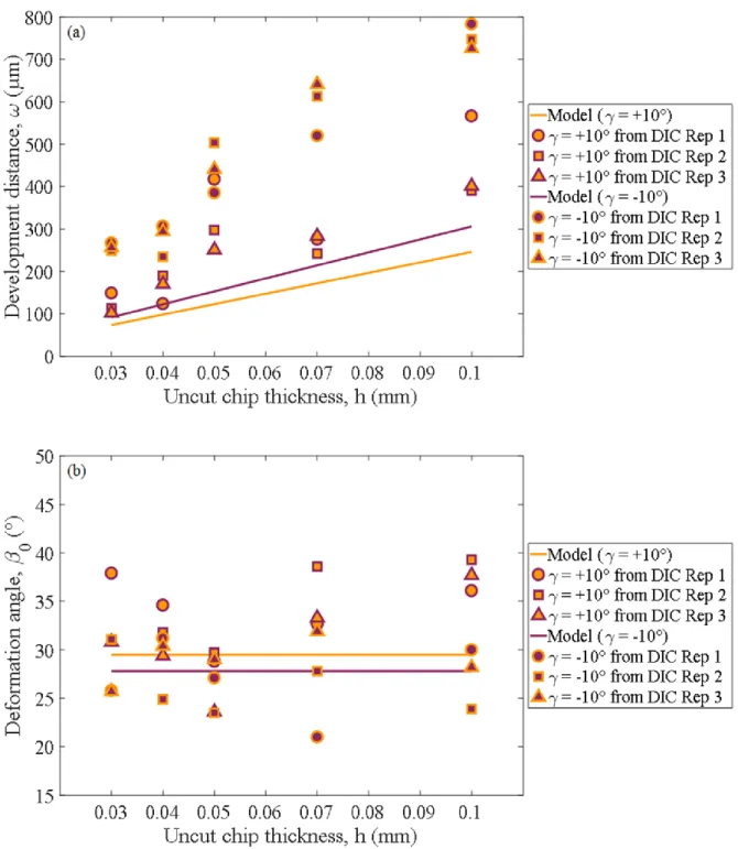
According to the model, predicted parameters influencing burr height are the burr
propagation distance and the deformation angle. Both model parameters are represented in Figure 18a and Figure 18b in function of the uncut chip thickness.
The burr propagation distance is underestimated while the predicted deformation angle is accurate. Propagation distance ω depends on the primary shear angle and deformation angle. The shear angle is predicted using an equation that does not take into account the influence of rake angle. Moreover, this parameter, presented in Figure 19, is overestimated for about 10° for both cases. Improving the prediction of this parameters has a major importance on the model accuracy. Nonetheless, if the shear angle becomes more realistic, it will affect the prediction of the deformation angle and the burr propagation distance. The deformation angle is determined using the assumptions of minimum of energy and energy conservation.
18
work provided for shearing and the work done for bending. After DIC analysis, it is
concluded that the localized deformation zone does not rotate. Hence, the work for bending may not be significant compared to shear and tension along the localized deformation zone generated during burr formation. As far as the primary deformation zone is concerned, the work done along this zone should be still considered since chip formation still occurs.
Conclusion
The present study aims to analyze burr formation mechanisms (with and without chamfer) using Digital Image Correlation at a common cutting speed, as an improvement of previous studies considering that issue (Ko and Dornfeld 1991; Chern and Dornfeld 1996; Hashimura et al. 1999b). A numerical simulation was performed with the aim of understanding the mechanisms behind burr with chamfer generation. Finally, experimental results are compared to an analytical model developed by Chern and Dornfeld (1996).
DIC analysis allows characterization of the initiation distance, the development distance and the deformation angle. The evolution of the localized high deformation is investigated. Its analysis does not correspond to the observation made by Chern and Dornfeld (1996) at low cutting speed on highly ductile material. It is observed in this study that the localized deformation zone during burr formation does not rotate, but it translates along the cutting direction while keeping the same angle. Burr root radius is driven by this displacement. In the case of burr with chamfer generation, the analysis of the principal strain fields provides information about the strain distribution before crack initiation. Quasi pure tension occurs around the cutting edge while compression occurs around the burr root. This explains the crack initiation while the tool moves forward. The analysis of stress triaxiality evolution during burr formation based on the numerical simulations confirms the observations made by DIC. A tensile stress zone expands from subsurface located under the tool cutting edge. A crack initiation occurs when this tensile stress zone reaches the tool cutting edge. The crack
19
propagates at the same time as both the cutting tool and the localized tensile stress zone move forward. Finally, at the very end of crack propagation, the compression zone generates a small burr.
To obtain better predictions, several issues can be improved in analytical model proposed by Chern and Dornfeld (1996), including:
- More recent shear angle models should be considered to obtain better shear angle prediction;
- The assumption of a rotation of the first deformation zone should be replaced by a displacement of this zone keeping the same orientation;
- Work done for primary shear during chip formation should be considered; - Stress triaxiality has an influence on the fracture strain, thus in cutting and burr
formation. To improve the prediction of burr with chamfer dimensions, a damage criterion using stress triaxiality to determine the fracture strain for the appropriate stress state could be used.
Acknowledgements
The authors would like to thank Bourgogne Franche-Comté Region for supporting this research project. The authors would like to thank to François Hild (LMT-Cachan) for his help on digital image correlation analysis and Stéphane Kapoujyan (master’s degree student) for the material mechanical characterization.
References
Abushawashi, Y.; Xiao, X.; Astakhov, V. (2013) A novel approach for determining material constitutive parameters for a wide range of triaxiality under plane strain loading conditions. International Journal of Mechanical Sciences, 74: 133–142.
Astakhov, V.P. (1998) Metal Cutting Mechanics. CRC Press.
Aurich, J.C.; Dornfeld, D.; Arrazola, P.J.; Franke, V.; Leitz, L.; Min, S. (2009) Burrs— Analysis, control and removal. CIRP Annals, 58(2): 519–542.
Baizeau, T.; Campocasso, S.; Fromentin, G.; Rossi, F.; Poulachon, G. (2015) Effect of rake angle on strain field during orthogonal cutting of hardened steel with c-BN tools. 15th
20
CIRP Conference on Modelling of Machining Operations (Vol. 31). Karlsruhe, Germany, Elsevier, 166–171.
Chern, G.-L. (2006) Study on mechanisms of burr formation and edge breakout near the exit of orthogonal cutting. Journal of Materials Processing Technology, 176(1–3): 152–157. Chern, G.-L.; Dornfeld, D.A. (1996) Burr/Breakout Model Development and Experimental
Verification. Journal of Engineering Materials and Technology, 118(2): 201–206. Gillespie, L.K.; Blotter, P.T. (1976) The Formation and Properties of Machining Burrs. Journal
of Engineering for Industry, 98(1): 66.
Hashimura, M.; Chang, Y.P.; Dornfeld, D. (1999) Analysis of Burr Formation Mechanism in Orthogonal Cutting. Journal of Manufacturing Science and Engineering, 121(1): 1–7. Hild, F.; Roux, S. (2012) Comparison of local and global approaches to digital image
correlation. Experimental Mechanics, 52(9): 1503–1519.
ISO 13715 (2017). Saga Web - NF ISO 13715, accessed September 12, 2018, available at
https://sagaweb-afnor-org.rp1.ensam.eu/fr-FR/sw/Consultation/Xml/1420769/?lng=FR&supNumDos=FA177597.
Iwata, K.; Ueda, K.; Okuda, K. (1982) Study of mechanism of burrs formation in cutting based on direct SEM observation. Journal of the Japan Society of Precision Engineering, 48(4): 510–515.
Johnson, G.R.; Cook, W.H. (1985) Fracture characteristics of three metals subjected to various strains, strain rates, temperatures and pressures. Engineering Fracture Mechanics, 21(1): 31–48.
Ko, S.-L.; Dornfeld, D.A. (1991) A Study on Burr Formation Mechanism. Journal of Engineering Materials and Technology, 113(1): 75–87.
Ko, S.-L.; Dornfeld, D.A. (1996a) Analysis of fracture in burr formation at the exit stage of metal cutting. Journal of Materials Processing Technology, 58(2–3): 189–200.
Ko, S.-L.; Dornfeld, D.A. (1996b) Burr formation and fracture in oblique cutting. Journal of Materials Processing Technology, 62(1–3): 24–36.
Kumar, S.; Dornfeld, D. (2003) Basic Approach to a Prediction System for Burr Formation in Face Milling. Journal of Manufacturing Processes, 5(2): 127–142.
Leopold, J.; Freitag, H.; Hoyer, K.; al, et (2005) Modeling and simulation of burr formation - State of the art and future trends. 8th CIRP International Workshop on Modeling of Machining Operations 2005. Proceedings, 73–83.
Merchant, M.E. (1945) Mechanics of the Metal Cutting Process. I. Orthogonal Cutting and a Type 2 Chip. Journal of Applied Physics, 16(5): 267–275.
Park, I.W.; Dornfeld, D.A. (1999) A Study of Burr Formation Processes Using the Finite Element Method: Part I. Journal of Engineering Materials and Technology, 122(2): 221–228.
Pottier, T.; GERMAIN, G.; CALAMAZ, M.; Morel, A.; COUPARD, D. (2014) Sub-millimeter measurement of finite strains at cutting tool tip vicinity. Experimental Mechanics, 54(6): 1031–1042.
Regel, J.; Stoll, A.; Leopold, J. (2009) Numerical analysis of crack propagation during the burr formation process of metals. International Journal of Machining and Machinability of Materials, 6(1/2): 54.
Régnier, T.; Fromentin, G.; D’Acunto, A.; Outeiro, J.; Marcon, B.; Crolet, A. (2018) Phenomenological Study of Multivariable Effects on Exit Burr Criteria During Orthogonal Cutting of AlSi Alloys Using Principal Components Analysis. Journal of Manufacturing Science and Engineering, 140(10): 101006-101006–10.
Régnier, T.; Fromentin, G.; Marcon, B.; Outeiro, J.; D’Acunto, A.; Crolet, A.; Grunder, T. (2018) Fundamental study of exit burr formation mechanisms during orthogonal cutting of AlSi aluminium alloy. Journal of Materials Processing Technology, 257: 112–122.
21
Rice, J.R.; Tracey, D.M. (1969) On the ductile enlargement of voids in triaxial stress fields∗. Journal of the Mechanics and Physics of Solids, 17(3): 201–217.
Sutton, M.A.; Orteu, J.J.; Schreier, H. (2009) Image Correlation for Shape, Motion and Deformation Measurements: Basic Concepts,Theory and Applications. Springer US.
22
Figures:
Figure 1: Model adapted from Ko and Dornfeld (1991) for burr initiation.
23 Figure 3: Experimental setup.
24
Figure 4: Selected images showing both types of burr formation: (a) without chamfer. (b) with chamfer (reference image is noted by ‘Ref’ and the image at burr initiation is noted by ‘i’).
25
Figure 5: ROI applied to the reference image (before cutting) and its respective grey level distribution (γ = -10°).
26
Figure 7: X-displacement field at burr initiation: (a) without chamfer; and (b) with chamfer. (c) Measured initiation distances for both types of burrs.
27
Figure 8: Major strain evolution between initiation and development. (a) Burr without chamfer. (b) Burr with chamfer.
28
Figure 9: Displacements and principal strain fields evolution during burr without chamfer formation (γ = -10°): (a) X displacement. (b) Major strain. (c) Minor strain.
29
Figure 10: Displacements and principal strain fields evolution during burr formation with chamfer (γ = +10°). (a) X displacement. (b) Maximum principal strain. (c) Minimum principal strain.
31
Figure 11: Strain state evolution during both types of burr formation and principal strain at the zones indicated in the images (where the equivalent strain is significant). (a) Burr without chamfer. (b) Burr with chamfer.
Figure 12: Boundary conditions and elements distribution for the numerical model.
32
Figure 14: Experimental fracture strain in function of stress triaxiality for ENAC-ALSi7Mg0.3 + 0.5Cu and its corresponding reduced Johnson-Cook fracture model (Johnson and Cook 1985).
Figure 15: Equivalent strain fields during burr development: (a) measured by DIC; and (b) simulated. The measured distribution corresponds approximately to the rectangular region indentified in figure 16b.
34
Figure 16: (a) Simulated equivalent plastic strain (𝜺̅) and (b) stress triaxiality (ƞ) during the burr formation with chamfer (h = 0.1 mm, γ = +10°).
Figure 17: Comparison between prediction (solid lines) and experiment (dots) for burr height and chamfer height. ‘From laser scan’ refers to the average measurements along the exit edge, scanned with the profilometer. ‘From hsc image’ refers to distances directly measured on the high-speed camera images.
35
Figure 18: Comparison between predicted and measured results for: (a) burr propagation distance and (b) deformation angle.
36
Figure 19: Comparison between predicted and experimental shear angle. Figure 1: Model adapted from Ko and Dornfeld (1991) for burr initiation. Figure 2: Burr formation process mechanisms (from Hashimura et al. (1999b)). Figure 3: Experimental setup.
Figure 4: Selected images showing both types of burr formation: (a) without chamfer. (b) with chamfer (reference image is noted by ‘Ref’ and the image at burr initiation is noted by ‘i’).
Figure 5: ROI applied to the reference image (before cutting) and its respective grey level distribution (γ = -10°).
Figure 6: Computation errors during burr formation. (a) Burr without chamfer. (b) Burr with chamfer. Figure 7: X-displacement field at burr initiation: (a) without chamfer; and (b) with chamfer. (c) Measured initiation distances for both types of burrs.
Figure 8: Major strain evolution between initiation and development. (a) Burr without chamfer. (b) Burr with chamfer.
Figure 9: Displacements and principal strain fields evolution during burr without chamfer formation (γ = -10°): (a) X displacement. (b) Major strain. (c) Minor strain.
Figure 10: Displacements and principal strain fields evolution during burr formation with chamfer (γ = +10°). (a) X displacement. (b) Maximum principal strain. (c) Minimum principal strain.
Figure 11: Strain state evolution during both types of burr formation and principal strain at the zones indicated in the images (where the equivalent strain is significant). (a) Burr without chamfer. (b) Burr with chamfer.
Figure 12: Boundary conditions and elements distribution for the numerical model. Figure 13 : Flow stress curves for ENAC-ALSi7Mg0.3 + 0.5Cu.
Figure 14: Experimental fracture strain in function of stress triaxiality for ENAC-ALSi7Mg0.3 + 0.5Cu and its corresponding reduced Johnson-Cook fracture model (Johnson and Cook 1985).
Figure 15: Equivalent strain fields during burr development: (a) measured by DIC; and (b) simulated. The measured distribution corresponds approximately to the rectangular region indentified in figure 16b.
Figure 16: (a) Simulated equivalent plastic strain (𝜺) and (b) stress triaxiality (ƞ) during the burr formation with chamfer (h = 0.1 mm, γ = +10°).
Figure 17: Comparison between prediction (solid lines) and experiment (dots) for burr height and chamfer height. ‘From laser scan’ refers to the average measurements along the exit edge, scanned with
37
the profilometer. ‘From hsc image’ refers to distances directly measured on the high-speed camera images.
Figure 18: Comparison between predicted and measured results for: (a) burr propagation distance and (b) deformation angle.
Figure 19: Comparison between predicted and experimental shear angle.
Tables:
Table 1: Mechanical properties of the work material.
PROPERTY
VALUE
(average [min; max]) Density (g/cm3) 2.66 Young Modulus (GPa) 78.5 [74.2; 82.6] Elongation at break (%) 2.1 [0.9; 3.9] Tensile Yield strength (MPa) 250.3 [243.9; 257.2] Tensile Ultimate strength (MPa) 295.6 [276.5; 317.1] Poisson ratio 0.33
38 Table 2: Cutting conditions including insert specifications.
PARAMETERS VALUES
Tool material HW-K20
General surface roughness of the rake face, Ra (µm)
0.8
Cutting speed, Vc
(m/min)
120
Uncut chip thickness, h (mm)
0.03; 0.04; 0.05; 0.07 and 0.10
Repetitions 3
Width of cut, b (mm) 4
Rake angle, γ (°) -10 and 10 Clearance angle, α (°) 10
Edge radius, rβ (μm) 10
39
Table 3: Comparison between predicted and measured results.
Measured (average values) Predicted
Cutting force (N) 382 to 387 256
Feed force (N) 189 to 198 97.6
Chip compression ratio 2.58 1.5
Chamfer depth (µm) 94 to 195 62
Chamfer height (µm) 217 to 315 277
Chamfer angle (°) 25 to 35 20.9
Burr height (µm) 20 to 59 6
Table 1: Mechanical properties of the work material. Table 2: Cutting conditions including insert specifications. Table 3: Comparison between predicted and measured results.