Handle ID: .http://hdl.handle.net/10985/8974
To cite this version :
Jean-Christophe LOISEAU, Jean-Christophe ROBINET, Stefania CHERUBINI, Emmanuel LERICHE - Investigation of the roughness-induced transition: global stability analyses and direct numerical simulations - Journal of Fluid Mechanics - Vol. 760, p.175-211 - 2014
Any correspondence concerning this service should be sent to the repository Administrator : archiveouverte@ensam.eu
Investigation of the roughness-induced
transition: global stability analyses and
direct numerical simulations
Jean-Christophe Loiseau
1,2†, Jean-Christophe Robinet
1Stefania Cherubini
1and Emmanuel Leriche
21
Laboratoire DynFluid, Arts et M´etiers ParisTech, Paris, France
2
Laboratoire de M´ecanique de Lille, Villeneuve d’Ascq, France (Received ?; revised ?; accepted ?. - To be entered by editorial office)
The linear global instability and resulting transition to turbulence induced by an iso-lated cylindrical roughness element of height h and diameter d immersed within an incom-pressible boundary layer flow along a flat plate is investigated using the joint application of direct numerical simulations and fully three-dimensional global stability analyses. For the range of parameters investigated, base flow computations show that the roughness element induces a wake composed of a central low-speed region surrounded by a three-dimensional shear layer and a pair of low- and high-speed streaks on each of its sides. Results from the global stability analyses highlight the unstable nature of the central low-speed region and its crucial importance in the laminar-turbulent transition process. It is able to sustain two different global instabilities: a sinuous and a varicose one. Each of these globally unstable modes are related to a different physical mechanism. While the varicose mode finds its root in the instability of the whole three-dimensional shear layer surrounding the central low-speed region, the sinuous instability turns out to be similar to the von K´arm´an instability in the two-dimensional cylinder wake and finds its root in the lateral shear layers of the separated zone. The aspect ratio of the roughness element plays a key role on the selection of the dominant instability. Indeed, whereas the flow over thin cylindrical roughness elements transitions due to a sinuous instability of the near-wake, for larger roughness element the varicose instability of the central low-speed region turns out to be the dominant one. Direct numerical simulations of the flow past an aspect ratio η = 1 (with η = d/h) roughness element sustaining only the sinuous instability have revealed that the bifurcation occurring in this particular case is supercritical. Finally, comparison of the transition thresholds predicted by global linear stability analyses with the von Doenhoff-Braslow transition diagram provides qualitatively good agreements. Key words:
1. Introduction
Understanding, predicting and eventually delaying the laminar-turbulent transition in boundary layer flows still is a challenging issue for researchers ever since the pioneering work by Ludwig Prandtl and his two students, Walter Tollmien and Hermann Schlichting. For small amplitude disturbances and supercritical Reynolds numbers, the linear stabil-ity theory predicts the slow transition process due to the generation, amplification and
shown that this natural transition could be promoted using spanwise invariant rough-ness elements. This earlier transition is related to the modified stability properties of the boundary layer flow developing downstream the roughness element. More precisely, this transition process is explained by the enhancement of the unstable TS waves due to mod-ifications of the flow’s properties in the downstream reversed flow and recovery regions. More recently, Perraud et al. (2004) have shown that the higher the two-dimensional roughness element, the closer to it does transition to turbulence take place. On the other hand, the influence of fully three-dimensional roughness elements on the transition to turbulence is very different. Indeed, whereas fully three-dimensional roughness elements hardly promote flow separation, they induce streamwise velocity streaks. It has been shown by Cossu & Brandt (2004) that these streaks act as stabilising the TS waves and thus delay the natural transition process. This delay of the transition to turbulence by fully three-dimensional roughness elements has been further confirmed experimentally by Fransson et al. (2004, 2005, 2006), using an array of cylindrical roughness elements. Though promising, this delay technique needs a careful choice of the main parameters of the setup, namely the Reynolds numbers, the shape and spacing of the roughness elements, as well as their height with respect to the thickness of the boundary layer. In fact, the previously mentioned authors have observed that, beyond a given threshold, the velocity streaks induced by the three-dimensional roughness elements can become themselves unstable yielding the flow to transition to turbulence right downstream the roughness elements.
It is known that in the presence of moderate to high environmental noise, free-stream disturbances can penetrate into the boundary layer and trigger by-pass transition. The developing perturbations no longer take the form of TS waves but of velocity streaks which are quasi-optimal disturbances (i.e. with the optimal perturbation being the one inducing the largest transient energy growth in the considered base flow). Because three-dimensional roughness elements also induce velocity streaks in the boundary layer, it is believed that such by-pass transition and fully three-dimensional roughness-induced transition share some connections. The formation process of these high- and low-speed streaks has been explained by Landahl (1990) and relies on the lift-up effect. The free-stream disturbances entering the boundary layer give birth to free-streamwise aligned counter-rotating vortices. Such vortices then transfer high-speed fluid from the outer part of the boundary layer toward the wall and low-speed fluid from the wall toward the outer region of the boundary layer. Due to this transfer of momentum, the resulting perturbation takes the form of high- and low-speed streaks. The dynamics of optimal streaks has been investigated by Andersson et al. (2001). These can potentially undergo a secondary instability taking the form of a sinuous modulation of the streaks when their amplitude exceeds approximately 26% of the free-stream velocity. Instability with respect to varicose perturbations has also been reported for optimal streaks having an amplitude larger than roughly 37% of the free-stream velocity. However, more recently, Konishi & Asai (2004) have shown experimentally that the stability properties of isolated streaks, as the ones induced by an isolated three-dimensional roughness element, are different from the ones of spanwise-periodic, optimal streaks as those considered in Andersson et al. (2001). In fact, even if one can carefully choose the shape and aspect ratio of an isolated roughness
2006), the shape of the induced streaks will be rather different, especially concerning the lateral ones, which would easily fade away in the absence of side vortices able to sustain them.
Concerning the flow past three-dimensional roughness elements and its transition to turbulence, Sedney (1972) has reviewed most of the literature available until the early 1970’s. The flow pattern induced by an isolated three-dimensional roughness element has been known for almost 60 years (Gregory & Walker 1955). When impinging the three-dimensional roughness element, the spanwise vorticity of the incoming boundary layer wraps around the protuberance thus creating horseshoe vortices. One of the most thorough investigations of the structure of such vortical structures has been carried out by Baker (1978), for an isolated cylindrical roughness mounted on a flat plate. As shown by Baker (1978), the number of horseshoe vortices wrapped around the roughness ele-ment, as well as their main features, mostly depend on the aspect ratio of the roughness element considered. However, in all of these cases, such horseshoe vortices give birth further downstream to quasi-aligned streamwise vortices. As already explained, due to the lift-up effect (Landahl 1990), these streamwise aligned vortices can trigger strong transient growth of the boundary layer streaks (Joslin & Grosch 1995), strong enough to yield their breakdown and subsequent transition to turbulence.
The receptivity of the boundary layer flow to an array of three-dimensional cylindri-cal roughness elements and the associated transient growth of the velocity streaks have been thoroughly investigated by various authors as Fischer & Choudhari (2004), Er-gin & White (2006), Fransson et al. (2004, 2005), as well as Denissen & White (2008, 2009). Their major finding is that the streamwise transient growth of the induced streaks roughly scales with the square of the roughness Reynolds number, Reh= UBl(xk, h)h/ν (UBl being the value of the Blasius velocity profile evaluated at the roughness element’s position xk and height h).
The crucial importance of the roughness Reynolds number in the roughness-induced transition to turbulence had already been outlined many years earlier. Indeed, as soon as the early 1960’s, Tani et al. (1962) had already observed experimentally that the tran-sition to turbulence in the wake of an aspect ratio η = 1 cylindrical roughness element is occurring in the vicinity of Reh= 600 almost independently of the other parameters characterising the flow (provided the roughness element is totally immersed within the boundary layer). Almost at the same time, von Doenhoff & Braslow (1961) have reviewed most of the experimental results available back then, obtained for roughness elements of different shape, height and spanwise spacings, and compiled them into a transition diagram correlating the aspect ratio of the roughness element to the roughness Reynolds number beyond which the induced flow would transition to turbulence. The von Doenhoff & Braslow (1961) diagram clearly shows that the fundamental parameters for predict-ing transition to turbulence past a roughness element are its aspect ratio and its height with respect to the Blasius boundary layer profile. In particular, the height of the rough-ness element appears to be fundamental for the development of streamwise streaks of finite amplitude and length. The crucial role of streaks in the onset of transition has been highlighted by Vermeersch (2009) and Arnal et al. (2011), who have developed a model grounded on optimal perturbation theory to determine transition to turbulence past roughness elements of any shape. In particular, they have conjectured that transi-tion occurs when the ratio of the shear stress generated by optimal streaks, with respect to the viscous stress, reaches a given critical value. Though promising, their approach relies on the strong assumption of quasi-parallelism of the flow induced by the three-dimensional roughness element, regardless of the separation zones which can be induced
is generated, creating relatively high- and low-speed streaks in the wake downstream of the bump. An investigation of the local stability of streamwise streaks developing past a smooth, large, isolated roughness element has been carried out by Piot et al. (2008). As-suming that the flow past the smooth roughness element evolves slowly in the streamwise direction, they have studied its local stability properties at each streamwise location just behind the roughness element, assessing the stabilizing effect of such a pre-streaky flow on the growth of TS waves. The same configuration has been studied very recently by Cherubini et al. (2013) from a global point of view. To investigate bypass transition in the presence of a large isolated bump, these authors have searched for the optimal per-turbation inducing the largest growth of disturbances over the fully three-dimensional flow field surrounding this smooth roughness element. In this three-dimensional frame-work, the optimal perturbation takes the form of a wavepacket-like structure initially localised in the vicinity of the separation line on the top of the roughness element and will eventually travel along the central low-speed streak induced by the roughness ele-ment. Interestingly enough, at small target times, this optimal perturbation exhibits a varicose symmetry, whereas at larger target times it exhibits a sinuous structure. It is worthy to note that for the geometry they have investigated, the varicose optimal per-turbation is the most efficient to trigger localised transition and induces hairpin vortices once non-linearities are taken into account. However, due to the linearly stable nature of the flow considered, the unsteadiness observed is not self-sustaining once these linear transients have been washed out from the computational domain. In the mean time, de Tullio et al. (2013) have investigated the roughness-induced transition in the case of a compressible boundary layer flow using the joint application of local stability analy-sis, parabolised stability equations and direct numerical simulations. These authors have shown that the flows they have investigated are much more convectively unstable, be it to varicose or sinuous perturbations, than the classic boundary layer flow. Moreover, for the sharp-edged rectangular roughness element they considered, the varicose perturbations exhibit larger temporal and spatial growth rates than their sinuous counterparts. Though they provide valuable insights into the linear dynamics of the flow, stability anal-yses as performed by Piot et al. (2008) (for bumps), de Tullio et al. (2013) (for rectangular roughness elements), and Denissen & White (2013) (for cylinders), rely on the strong as-sumption of a nearly parallel flow. However, the flow past three-dimensional roughness elements exhibits some reversed flow regions where such parallel assumption can not hold. As a consequence, for such class of flows, stability analyses relying on a parallel flow hypothesis totally discard the influence of the region in the vicinity of the roughness element on the stability properties of the overall flow field which, as seen by Fransson et al. (2005), appears to be the region triggering the unsteadiness. To circumvent this major drawback and to fully capture the instability mechanisms, one then has to turn to a fully three-dimensional global stability framework for which no such parallel assumption is required. Since the number of degrees of freedom involved in such formulation of the stability problem is extremely large, fully three-dimensional global stability analysis still is nowadays a heavy computational task. Hopefully, with the increase of computational ressources over the past decade and the recent popularisation of new eigenvalues algo-rithms (Edwards et al. 1994; Bagheri et al. 2009a), investigation of the linear stability
of a jet in cross flow, Bagheri et al. (2009b) and Ilak et al. (2012) have shown that fully three-dimensional global stability analysis is able to provide a better understanding of the underlying instability mechanisms. To our knowledge, no such global stability analy-sis has ever been attempted on the flow past a three-dimensional roughness element. The aim of the present work is to provide new insights on the roughness-induced transition using these new developments in the global stability theory. Indeed, it is believed that fully three-dimensional global stability analysis can help us addressing several questions among which:
(i) Can the varicose and sinuous instability mechanisms found by local stability anal-yses, as well as the critical Reynolds number measured in experiments and numerical simulations, be accurately recovered using a fully three-dimensional global approach?
(ii) Can one link the roughness-induced transition to a global instability of the flow and not only to transient growth and associated convectively unstable perturbations as widely accepted until now?
(iii) Is it possible to predict the flow’s non-linear patterns and dynamics using pieces of information stemming from linear analyses?
The case of a cylindrical roughness element immersed within a laminar boundary layer flow developing along a flat plate is investigated. The present paper is structured as follows: first, in section 2 the problem under consideration and the numerical methods used are presented. In section 3, the experimental case investigated by Fransson et al. (2005) is reproduced numerically and its global instability is investigated. In section 4, a parametric investigation is carried out, highlighting two instability mechanisms, a sinuous and a varicose one, arising for roughness elements of different aspect ratio. In section 5, direct numerical simulations revealing the non-linear evolution of these instabilities as well as the criticality of the bifurcation associated with the sinuous one are presented. Finally, in section 6 concluding remarks are provided.
2. Problem formulation
2.1. Governing equations
The dynamics of a three-dimensional incompressible flow are described by the incom-pressible Navier-Stokes equations:
∂U ∂t + (U · ∇)U = −∇P + 1 Re∆U ∇ · U = 0 (2.1)
where U = (U, V, W )T is the velocity vector and P the pressure term. Dimensionless variables are defined with respect to the height h of the cylindrical roughness element and to the free-stream velocity U∞. Therefore, the Reynolds number is defined as Re = U∞h/ν, with ν being the kinematic viscosity. Concerning the coordinate system, x, y and z are defined as the streamwise, wall-normal and spanwise directions, respectively, with x having its origin at the leading edge of the flat plate. However, since the domains used in this work do not include the leading edge of the flat plate, it is convenient to define a shifted streamwise axis X = x − xk, having its origin at the location xk of the roughness element along the flat plate. A sketch of the computational domain considered is depicted on figure 1, along with this roughness-centered coordinate system. The cylindrical roughness element, having diameter d and height h, is thus centred in
d h Lz l Lx δ 0
Figure 1.Sketch of the computational domain under consideration. The parameters defining the geometry take the following values: h = 1, l = 15 and (Lx, Ly) = (105, 50). Only the
roughness element’s diameter d will be varied and the spanwise dimension of the domain Lz.
90), a wall-normal extension of Ly= 50, whereas the spanwise extent Lzwill be varied in the different computations as specified in the next sections. In particular, in most of the computations, the spanwise domain length is chosen in order to make sure the roughness element behaves as being isolated (von Doenhoff & Braslow 1961), by scaling it with respect to the aspect ratio of the roughness element, η = d/h.
The following boundary conditions have been applied:
• at the inlet (Xin= −15), a Dirichlet boundary condition is imposed on the velocity. • at the outlet (Xout= 90), a Neumann boundary condition is imposed on the velocity ∇U · x = 0;
• on the spanwise end planes (zside= ±Lz/2), periodic boundary conditions are im-posed for the three components of the velocity vector;
• at the upper boundary (ytop= 50), the following conditions are applied: U = 1 and ∂V /∂y = ∂W/∂y = 0;
• finally, a no-slip boundary condition is imposed on the flat plate and the walls of the roughness element.
Note that two other domains extending down to Xout = 30 and Xout = 60 in the
streamwise direction have been considered, whereas the inlet of the domain has been kept at a streamwise distance l = 15 upstream the center of the roughness element (see figure 1). However, in order to present results independent of the domain size, only the longest domain (i.e. Xout = 90) will be considered in the present work, as discussed in detail in Appendix B providing a numerical convergence analysis.
Calculations have been performed using the code Nek5000 developed at Argonne Na-tional Laboratory by Fischer et al. (2008). Spatial discretisation is done by a Legendre spectral elements method with polynomials of order 12. Depending on the aspect ratio considered, the number of spectral elements in the mesh ranges from 10 000 for η = 1 up to 18 800 for η = 3. The convective terms are advanced in time using an extrapolation of order 3, whereas for viscous terms a backward differentiation of order 3 is used, resulting in the time-advancement scheme labelled BDF3/EXT3.
η 1 2 3 Re 1000 − 1500 750 − 1000 500 − 800
χ 0.05 − 0.1 0.05 − 0.1 0.05 − 0.1
ωc 0.25 0.5 0.5
Table 1.Typical values of the parameters χ and ωc used in the selective frequency damping
as to compute the base flows for the different cases considered.
2.2. Base flows computation
Seeking for stationary solutions Ub = (Ub, Vb, Wb)T of the Navier-Stokes equations is a pre-requisite to the stability analysis performed in this work. Such solutions, also called base flows or fixed points of system (2.1), have been computed using the selective fre-quency damping (SFD) approach introduced by Akervik et al. (2006). This technique enables a damping of the oscillations of the unsteady part of the solution using a tempo-ral low-pass filter. This is achieved by adding a forcing term to the right-hand side of the Navier-Stokes equations and extending the system (2.1) with an equation for the filtered state ¯U. The extended system is then governed by the following set of equations:
∇ · U = 0 ∂U ∂t = −(U · ∇)U − ∇P + 1 Re∆U − χ(U − ¯U) ∂ ¯U ∂t = ωc(U − ¯U) (2.2)
with χ being the gain of the filter and ωc its cutting circular frequency. The choice of these two parameters is crucial for the computation of unstable base flows: the gain χ has to be positive and larger than the growth rate σ of the instability one aims to quench, whereas ωc has to be lower than the eigenfrequency ω of the instability (usually ωc= ω/2). It can be shown that this extended system converges toward the equilibrium solution Ub = (Ub, Vb, Wb)T of the Navier-Stokes equations. Table 1 provides typical values of χ and ωc that have been used for the base flows computations. For further details, the reader is referred to Akervik et al. (2006).
Since the computational domain does not include the leading edge of the flat plate, a Blasius velocity profile is imposed at inlet points. The imposed profile is chosen by requiring that the theoretical Blasius boundary layer displacement thickness, δ∗, that the flow would have at (X, z) = (0, 0) in the absence of the roughness element, has a prescribed value with respect to the roughness height. The prescribed values of δ∗, as well as the associated values of the displacement thickness Reynolds number, Reδ∗ = U∞δ∗/ν,
will be given in the next sections, allowing a comparison with the configurations used in previous studies.
2.3. Three-dimensional global stability analysis
Linear stability analysis enables the investigation of the asymptotic time evolution of infinitesimal perturbations in the vicinity of a given fixed point of the original system. In the present case, one needs to use the linearised Navier-Stokes equations. The linearised dynamics of such infinitesimal perturbations evolving onto the base flow Ubare governed
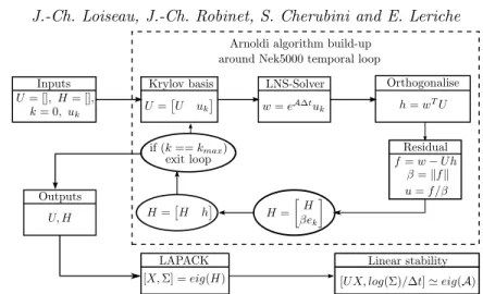
Figure 2.Block-diagram of the Arnoldi algorithm used.
by the following set of equations: ∂u
∂t = −(u · ∇)Ub− (Ub· ∇)u − ∇p + 1
Re∆u
∇ · u = 0
(2.3)
where u = (u, v, w)T is the perturbation velocity vector and p the perturbation pressure. This set of equations is subject to the same boundary conditions as system (2.1) with the inlet Dirichlet boundary condition being a zero-velocity condition. Introducing the perturbation state vector q = (u, p)T, one can recast the previous set of equations into the following linear dynamical system form:
B∂q∂t = J q (2.4)
where B is a singular mass matrix, and J is the Jacobian matrix of the Navier-Stokes equations (2.1) linearised around the fixed point Ub. Once projected onto a divergence-free vector space, this system simply reads:
∂u
∂t = Au (2.5)
with A being the projection of the Jacobian matrix J onto the divergence-free vector space. Because the number of degrees of freedom involved in the computation is far too large to enable explicit storage of A and thus direct computation of its eigenvalues, a time-stepper approach as introduced by Edwards et al. (1994) and Bagheri et al. (2009a) is used. This method, based on an Arnoldi algorithm and on the formal solution u(∆t) = eA∆tu
0to equation (2.5), aims at computing the eigenpairs of the exponential propagator
M = eA∆t instead of those of the Jacobian matrix A. Indeed, though the Jacobian
matrix A cannot be explicitly computed, the action of the exponential propagator onto a given vector can be easily approximated by time-marching the linearised Navier-Stokes equations from t = 0 to t = ∆t. At iteration k, the basic Arnoldi iteration thus reads:
MVk ≃ VkHk (2.6)
with Vk being an orthonormal set of vectors spanning a Krylov subspace of dimension k onto which M is projected, and Hk being the associated projection. The Hessenberg
Case 1 Case 2 Case 3 Case 4 δ∗(x
k) 0.6026 0.5547 0.5425 0.5310
Reδ∗ 281 305 312 319
Re 466 550 575 600
Stability Stable Stable Unstable Unstable
Table 2.Summary of the different cases considered in Section 3. For all of them, the roughness elements are located at a distance xk= 57.14 from the leading edge, separated by Lz = 10 and
have an aspect ratio η = 3.
matrix Hk resulting from this Arnoldi iteration is a small k × k matrix whose eigenpairs (Σ, X), also called Ritz pairs, can be directly computed and are a good approximation of those of M. Ritz pairs are linked to the eigenvalues and eigenvectors (Λ, Q) of the Jacobian matrix A by the following relationship:
Λ = log(Σ)
∆t , Q = VX (2.7)
with Λ = σ+iω, σ being the growth rate and ω the circular frequency. The block-diagram of the complete algorithm is depicted on figure 2. It can be seen as an alternative to the algorithm proposed by Barkley et al. (2008) where the exit condition has been simplified. All of the results presented throughout this paper were obtained using a Krylov subspace of dimension 500 and a sampling period ∆t = 0.625 enabling good convergence of the eigenvalues with circular frequency equals to 2.5 and lower. Concerning the convergence of the procedure with respect to other numerical parameters, more details are given in Appendix B.
3. The Fransson experiment
Following the theoretical work by Cossu & Brandt (2004), Fransson et al. (2004, 2005, 2006) have conducted a series of experiments demonstrating the ability for finite am-plitude streaks to stabilise the Tollmien-Schlichting waves and thus delay the natural transition of the boundary layer flow. With this aim, they have placed an array of rough-ness elements, having an aspect ratio η = 3, located at xk = 57.14 from the leading edge of a flat plate and separated one from another by a spanwise distance Lz = 10 (Frans-son et al. 2005). Despite the stabilising effect of the streaks on the TS waves, transition was however observed to take place right downstream the roughness elements beyond a critical Reynolds number. In this section, the case described by Fransson et al. (2005) is reproduced numerically, in order to ascertain that fully three-dimensional global insta-bility analysis is able to predict with reasonable accuracy the critical Reynolds number experimentally obtained by the previously mentioned authors. The prescribed Reynolds numbers as well as the displacement thickness δ∗(x
k) are given in table 2. 3.1. Base flow
Figure 3 depicts the base flow obtained for (Re, Reδ∗, η) = (466, 281, 3), i.e. the same
setup as the reference one in Fransson et al. (2005). It exhibits the two major features of all the steady solutions that have been investigated within the present work: an upstream and a downstream reversed flow region (visualised by the Ub = 0 isosurface in the left frame), as well as a system of multiple vortices stemming from the upstream recirculation zone, wrapping around the roughness element and eventually getting almost aligned
(a) (b)
Figure 3.Computed base flow for (Re, Reδ∗, η) = (466, 281, 3). (a) Visualisation of the vortical
system using streamlines and isosurfaces of the upstream and downstream reversed flow regions (visualised by the Ub= 0 isosurface). (b) Close-up of the upstream vortical system highlighted
by streamlines in the symmetry plane coloured with the velocity magnitude.
with the streamwise direction of the flow as shown by the streamlines. The topology of this upstream vortical system has been investigated experimentally by Baker (1978) and exhibits between one and three counter-rotating vortex pairs. According to Baker (1978), the particular vortical topology chosen by the flow essentially depends on the Reynolds number and on the ratio of the roughness element’s diameter d over the boundary layer displacement thickness δ∗. This vortical system can be seen on figure 3(b) depicting streamlines in the symmetry plane. The impact of this vortical system on the boundary layer flow is as follows:
(i) Upstream the roughness element, all of the vorticity is in the spanwise direction. (ii) Once the flow encounters the roughness element, the upstream spanwise vorticity rolls up, forming the vortical system observed in figure 3(b).
(iii) It then wraps around the roughness element and is transferred into streamwise vorticity further downstream thus creating the legs of the horseshoe vortices.
The legs of these horseshoe vortices being streamwise-aligned vortices, high speed fluid is transported from the outer region of the boundary layer toward the wall, whereas low speed fluid is transported away from the wall toward the outer region of the bound-ary layer. This transport of momentum, known as the lift-up effect, thus gives birth to streamwise velocity streaks (Landahl 1990).
Figure 4 depicts the spatial distribution of the central low-speed region and outer streaks induced by the array of roughness elements at various streamwise stations. These streaks have been identified using the deviation of the base flow streamwise component from the corresponding Blasius boundary layer flow (UBl), as used by Fischer & Choud-hari (2004), i.e. ¯u = Ub−UBl. As shown on figure 4(a), the roughness element generates a central low-speed region created by the streamwise velocity deficit induced by the rough-ness element and a pair of high- and low-speed streaks induced by the legs of the primary horseshoe vortex on each side. On the one hand, the central low-speed region appears to fade away relatively rapidely in the streamwise direction, while on the other hand the outer pairs of streaks appear to sustain over quite a long distance. This can be better visualised on figures 4(b) to (d) depicting contours of the streamwise velocity deviation in various X = constant planes. It clearly appears from these figures that, while the amplitude of the central low-speed region has dramatically decreased as soon as X = 40, the amplitude of the outer low- and high-speed streaks varies very little. Such behavior has already been observed experimentally by Fransson et al. (2004) (see figure 2 of the cited paper).
(a)
(b) X = 20 (c) X = 40 (d) X = 80
Figure 4.Streamwise evolution of the streaks induced by the array of roughness elements for (Re, Reδ∗) = (466, 281): top view of the ¯u = ±0.3 surfaces (black and white), with ¯u = Ub−UBl
being the deviation of the base flow from the Blasius boundary layer flow (a); slices extracted at X = 20 (b), X = 40 (c) and X = 80 (d). The shaded contours range from ¯u = 0.3 (red) to ¯
u = −0.3 (blue), whereas the solid lines depict the base flows streamwise velocity isocontours from Ub= 0.1 to 0.99.
3.2. Global stability
In order to investigate the early transition observed in the experiment (Fransson et al. 2005), global stability analyses of various base flows are conducted. All of the cases considered are reported in table 2. Figure 5 depicts the spectra of eigenvalues for Re =
550 (Reδ∗ = 305) and Re = 575 (Reδ∗ = 319). It is clear from these eigenspectra
that the flow experiences a Hopf bifurcation for 550 < Rec < 575 due to an isolated pair of complex conjugate eigenvalues of the linearised Navier-Stokes operator moving into the upper-half complex plane. A linear interpolation provides a critical Reynolds number Rec = 564 ((Reδ∗)c = 309) only 6% larger than the critical Reynolds number
experimentally obtained by Fransson et al. (2005). This good agreement for the value of the critical Reynolds number strongly suggests that the transition observed in the experiment might be the consequence of a three-dimensional global instability of the flow. Comparison of the dominant frequency in the flow dynamics however turned out to be unconclusive essentially because the frequency reported by Fransson et al. (2005) has been measured far beyond the end of the computational domain considered herein
(X ≃ 175 compared to Xout = 90).
The shape of the associated unstable global mode is depicted on figure 6. As one can see on figure 6(a), this mode takes the form of streamwise alternated patches of positive and negative velocity exhibiting a varicose symmetry with respect to the spanwise mid-plane. To get a better insight of the structure of the mode and of its location with respect to the base flow’s features, figure 6 provides slices of its spatial support in the X = 23 (b) and the X = 40 (c) planes. The mode is identified using its streamwise velocity contours (shaded) whereas the solid black lines depict the baseflow Ub isocontours. These figures make it clear that, though the mode is initially located along the central low-speed region, it then contaminates almost the whole spanwise extent of the domain before fading away for X > 60. Moreover, for all of the streamwise planes considered, the maximum of the mode is located along the shear layers delimiting the central low-speed region and the streaks.
Figure 5.Eigenspectra of the linearised Navier-Stokes operator. Blue dots show the eigenvalues for (Re, Reδ∗) = (550, 305), whereas green triangles show the ones for (Re, Reδ∗) = (575, 312).
(a)
(b) X = 23 (c) X = 40
Figure 6. Visualisation of the streamwise velocity component of the leading unstable global mode at (Re, Reδ∗) = (575, 312). (a) Top view of isosurfaces depicting ±10% of the mode’s
maximum streamwise velocity. Slices in the (b) X = 23 plane (i.e., where the mode achieve its maximum amplitude) and in the (c) X = 40 plane. Both figures (b) and (c) have been normalised by the local maximum velocity. The solid lines depict the base flows streamwise velocity isocontours from Ub= 0.1 to 0.99.
4. Parametric investigation
In order to get a better understanding of the physical mechanisms underlying the roughness-induced transition, a parametric investigation is conducted. As to avoid the potential interaction between roughness elements, the spanwise extent of the computa-tional domain has been changed from Lz= 10 to Lz= 8η (with η being the aspect ratio of the roughness element considered) such that they behave as being isolated no matter the aspect ratio considered. Moreover, for the sake of clarity, the theoretical displace-ment thickness of the incoming Blasius boundary layer at the position of the roughness element is kept equal to δ∗(x
k) = 0.6883 (the boundary layer thickness being fixed at δ99(xk) = 2) throughout this investigation. This allows to isolate the influence of changes in the Reynolds number only and not a mixed combination of changes in the Reynolds number and displacement thickness at the same time. Finally, the aspect ratio η of the roughness elements considered will be varied from η = 0.85 up to η = 3, while the Reynolds number ranges from Re = 600 up to Re = 1250. Table 3 summarises most of the different cases treated during this parametric investigation.
η 1-3 1-3 1-3 1-2 1-2 1 1 Re 600 700 800 900 1000 1100 1250 xk 96 112 128 144 160 176 200
Reδ∗ 413 482 551 620 688 757 860
Table 3.Location xk of the roughness element along the flat plate such that δ∗(xk) = 0.6883
and the associated Reynolds numbers Re, Reδ∗ for most of the different cases considered in
Section 4’s parametric investigation.
4.1. Base flow 4.1.1. Influence of the Reynolds number
The influence of the Reynolds number Re on the base flow can be assessed from figures 7 and 8. Figures 7(a) and (b) provide slices of the streamwise velocity component of the base flow in the symmetry plane for (Re, η) = (600, 1) and (Re, η) = (1250, 1), respectively. It can be seen that when increasing the Reynolds number, the shape of the reversed flow regions remains almost unchanged. The main impact on the flow of an increase of the Reynolds number, and hence a decrease of the effect of viscosity, is however to strengthen the gradients as can be assessed from the stronger deformation of the iso-contours in figure 7(b). Increasing the Reynolds number also has an effect on the streaks induced by the vortical system identified previously. As can be seen on figure 8(a) in the lower Reynolds number case, the central low-speed streak induced by the roughness element’s blockage is fading away quite rapidly in the streamwise direction and one can even observe a merging of the two outer high-speed streaks resulting in only three streaks near the outflow: a central high-speed streak flanked with two low-speed ones. The merging of the high-speed streaks and the resulting pattern near the outflow can be better observed by visualizing the streamwise velocity contours on different X = constant planes, as provided in figure 9(a). A very similar behaviour has already been observed experimentally by Fransson et al. (2004) in a highly subcritical configuration. On the other hand, in the higher Reynolds number case shown in figures 8(b) and 9(b), the decrease of the viscosity’s effect allows the central low-speed region to sustain over a much longer streamwise extent and prevents, at least in the computational domain considered, the merging of the two high-speed streaks.
In both cases, the amplitude of the different streaks has been measured from X = 10, i.e. sufficiently far from the roughness element such that the strongly non-parallel effects induced by the reversed flow region can be discarded. Though the amplitude of the central low-speed region decays monotically in the streamwise direction for both cases, the initial amplitudes are quite different: miny,z(¯u) = −0.21 for Re = 600 and miny,z(¯u) = −0.47 for Re = 1250 at the streamwise position X = 10. On the other hand, the amplitude of the outer streaks varies between ±0.14 for Re = 600 and roughly ±0.3 for Re = 1250. From the work of Andersson et al. (2001), it would thus appear that the Re = 600 case is stable while the Re = 1250 case might be prone to streaks instability.
4.1.2. Influence of the aspect ratio
Figures 10(a) and (b) provide slices of the streamwise component of two base flows in the spanwise mid-plane obtained for the same Reynolds number and two different aspect ratios, namely (Re, η) = (600, 2) and (Re, η) = (600, 3), respectively. As one could have expected, due to the larger blockage induced by the roughness element, the reversed flow
Figure 7.Slices in the symmetry plane of different base flows. The dashed red line depicts the spatial extent of the reversed flow regions, whereas the thin solid black lines are the streamwise velocity contours ranging from 0.1 up to 0.99.
(a) (Re, η) = (600, 1), ¯u = ±0.075
(b) (Re, η) = (1250, 1), ¯u = ±0.2
Figure 8.Top view of the streaks induced by the roughness elements. Low-speed (white) and high-speed streaks (black) are depicted using isosurfaces of the streamwise velocity deviation of the baseflows from the theoretical Blasius boundary layer flow, ¯u = Ub−UBl.
(a) (Re, η) = (600, 1)
(b) (Re, η) = (1250, 1)
Figure 9.Visualisation of the streaks pattern in several different streamwise planes. On fig-ure (a), the color table ranges from ¯u = −0.2 (blue) to ¯u = 0.2 (red), while it ranges from ¯
u = −0.4 (blue) to ¯u = 0.4 in figure (b). The solid lines depict the base flows streamwise velocity isocontours from Ub= 0.1 to 0.99.
regions (depicted by the dashed red line) in the case of the η = 3 roughness element have a longer upstream and downstream extent than for the roughness elements of aspect ratio η = 1 and 2 (compare with figure 7(a) as well). Moreover, increasing the roughness element’s aspect ratio also slightly strengthens the gradients of the base flows. It is also worth noting that, when increasing the spanwise blockage given by the cylinder, more and
(a) (Re, η) = (600, 2) (b) (Re, η) = (600, 3)
Figure 10.Slices in the symmetry plane of different base flows. The dashed red line depicts the spatial extent of the reversed flow regions, whereas the thin solid black lines are the streamwise velocity contours ranging from 0.1 up to 0.99.
(a) (Re, η) = (600, 2), ¯u = ±0.2
(b) (Re, η) = (600, 3), ¯u = ±0.2
Figure 11.Top view of the streaks induced by the roughness elements. Low-speed (white) and high-speed streaks (black) are depicted using isosurfaces of the streamwise velocity deviation of the baseflows from the theoretical Blasius boundary layer flow, ¯u = Ub−UBl.
more upstream spanwise vorticity has to wrap around the roughness element, influencing the strength of the vortical system identified previously and, hence, the amplitude of the induced low- and high-speed streaks further downstream. These can be visualised on figure 11 where the deviation from the theoretical Blasius boundary layer of the steady equilibrium solutions for (Re, η) = (600, 2) and (Re, η) = (600, 3) are shown. Though for the present flows no merging of the high-speed streaks is observed, increasing the aspect ratio of the roughness element allows once again the central low-speed region to sustain on a longer streamwise extent indicating that the amplitude of the streaks is stronger.
As previously, the amplitude of the different streaks has been measured from X = 10 such that one can almost neglect the strongly non-parallel influence of the roughness element. While the central low-speed region has an amplitude of −0.4 at X = 10 for the η = 2 roughness element, its amplitude is −0.54 for the η = 3 case. However, the amplitude of the outer streaks roughly varies between ¯u = ±0.27, for η = 2, and ¯u = ±0.4, for η = 3. Once again, from the work of Andersson et al. (2001), it would thus appear that both cases might be prone to streaks local instabilities.
(a) (Re, η) = (600, 2)
(b) (Re, η) = (600, 3)
Figure 12.Visualisation of the streaks pattern in several different streamwise planes. The color table ranges from ¯u = −0.4 (blue) to ¯u = 0.4 (red). Solid lines depict the base flows streamwise velocity isocontours from Ub= 0.1 to 0.99.
4.2. Global stability
Figure 13 depicts the eigenspectra obtained for three of the cases considered. For all of them, the flow experiences a Hopf bifurcation due to an isolated complex conjugate pair of eigenvalues moving toward the upper-half complex plane. These isolated modes show a different type of structure depending on the aspect ratio considered. In particular, a sinuous global mode is observed for η = 0.85 and η = 1 (see the green dot in figure 13 (a)), whereas a varicose mode is obtained for η = 2 and η = 3 (see figures 13(b-c)). Shortly below, all these isolated eigenvalues are followed by a branch of modes exhibiting exclusively a varicose symmetry. For η = 3, this branch is closer to the isolated mode, so that a second unstable mode can be observed already at Re = 700. However, since the frequency and the structure of these two unstable modes are very similar, this does not result in strong changes on the related route to transition. It is worthy to notice that, whereas the isolated eigenvalues do not seem to be to very sensitive to the streamwise extent of the computational domain (provided Xout >60), the branches of eigenvalues on the other hand appear to be extremely sensitive and tend to move toward the upper-half complex plane as the streamwise length of the domain is reduced. For the longest domain considered (i.e. Xout = 90), table 4 provides the critical Reynolds numbers and the symmetry of the associated leading global mode for roughness elements of various aspect ratio η. Figure 14 depicts the leading unstable mode for each of the aspect ratios considered, at different Reynolds numbers. Since for all of these modes the streamwise component is at least almost 4 times larger than the other components, only the real part of this component is depicted. As can be seen, all the modes are mostly localised along the central low-speed region, differently from the case of non-isolated cylinder analysed in the previous section for which a large part of the mode migrates on the outer streaks downstream of the roughness element. The crucial importance of such low-speed regions in the roughness-induced transition process to turbulence has already been underlined by previous studies such as the experimental work by Asai et al. (2002, 2007), or the numerical investigation by Brandt (2007) and Denissen & White (2013). More recently, several different authors have observed a similar behaviour in the case of roughness-induced compressible boundary layer flows (Bernardini et al. 2012; Balakumar & Kegerise 2013; Iyer & Mahesh 2013; de Tullio et al. 2013; Subbareddy et al. 2014).
ω σ 0 0.5 1 1.5 2 -0.04 -0.02 0 0.02 0.04 (a) (Re, η) = (1200, 1) ω σ 0 0.5 1 1.5 -0.04 -0.02 0 0.02 0.04 (b) (Re, η) = (900, 2) ω σ 0 0.5 1 1.5 -0.04 -0.02 0 0.02 0.04 (c) (Re, η) = (700, 3) Figure 13. Spectrum of eigenvalues for different cases considered in the present work. Red
squares denote varicose modes whereas the green dot stands for a sinuous one.
η 0.85 1 2 3 Fransson et al. (2005) Rec 910 1040 805 656 564
Rec
h 712 813 630 513 519
Symmetry S S V V V
Table 4.Critical Reynolds number Recand symmetry of the associated leading unstable global
mode for various aspect ratio η. S stands for a sinuous global mode, and V for a varicose one.
It is obvious from table 4 and figure 14 that an exchange of symmetry of the leading unstable global mode occurs as the aspect ratio of the roughness element is increased. In-deed, whereas sinuous modes are found to be the dominant instability for thin cylindrical roughness elements (η 6 1), the varicose global instability turns out to be the dominant one when roughness elements of larger aspect ratio (η > 2) are considered. This exchange of symmetry of the leading unstable mode beyond a given threshold of the roughness el-ement’s aspect ratio had already been underlined experimentally by Sakamoto & Arie (1983) and Beaudoin (2004). The former authors have investigated the nature of the vortices shed periodically from prismatic and cylindrical roughness elements immersed within a turbulent boundary layer. For thin roughness elements, they have reported a shedding of von K´arm´an (sinuous) vortices, whereas they have labelled vortices shed from larger roughness elements as being arch-type vortices exhibiting a varicose symme-try. Though the present setup is different, due to the laminar nature of the incoming boundary layer flow, results from global stability analyses regarding the spatial structure of the dominant eigenmode are in qualitatively good agreement with their experimental observations, as it will shown in more detail in Section 5 by direct numerical simulations.
4.2.1. Analysis of the modes
Regarding the sinuous mode, its spatial structure has already been shown in fig-ure 14(a) and (b). As one can see, it consists in positive and negative patches of veloc-ity mostly localised along the central low-speed region. Its streamwise and wall-normal components are exhibiting a sinuous symmetry with respect to the spanwise mid-plane, whereas its spanwise component exhibits a varicose symmetry with respect to the same plane (not shown). To get a better insight of the structure of the mode and of its location with respect to the base flow’s features, figure 15(a) provides a slice of it in the X = 25
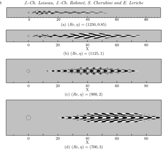
(b) (Re, η) = (1125, 1)
(c) (Re, η) = (900, 2)
(d) (Re, η) = (700, 3)
Figure 14. Real part of the leading unstable mode streamwise component with increasing roughness element’s aspect ratio η from top to bottom, and different Reynolds numbers indicated within the figure. The isosurfaces depict u = ±10% of the maximum amplitude of the modes, whereas open black circles denote the location of the roughness elements.
plane for (Re, η) = (1125, 1). The mode is identified using its streamwise velocity con-tours (shaded) whereas the solid black lines depict the baseflow Ubisocontours. The fully three-dimensional shear layer developing around the velocity streaks, here depicted by the red dashed line, is identified using the points of null curvature in the Ubdistribution, i.e. ∂2
Ub/∂y2+ ∂2Ub/∂z2= 0. It can be seen that the regions of maximum amplitude of the mode are located on the flanks of the central low-speed region along its shear layer. Such particular location, where the wall-normal and spanwise gradients of the base flow are relatively strong, let us think that this sinuous global instability is likely to extract the energy for its growth from the transport of these two shears along the central low-speed region, as it will be shown in detail in subsection 4.3.
The second type of global instability identified from figures 14(c) and (d) is a varicose global instability. As for its sinuous counterpart, this second family of unstable modes is essentially localised along the central low-speed region and consists in streamwise al-ternated patches of positive and negative velocity. The major difference is however the symmetry of the mode: its streamwise and wall-normal components now exhibit a vari-cose symmetry with respect to the spanwise mid-plane, whereas its spanwise component exhibits a sinuous symmetry (not shown). As previously, in order to gain a better
under-(a) (Re, η) = (1125, 1) (b) (Re, η) = (850, 2)
Figure 15. Slice of the streamwise component of the sinuous unstable global mode (a) and varicose global mode (b) in the X = 25 plane identified by the shaded red and blue contours. Solid lines depict the base flows streamwise velocity isocontours from Ub= 0.1 to 0.99, whereas
the red dashed line stands for the location of the shear layer identified by the points of null curvature (i.e. ∂2 Ub/∂y 2 + ∂2 Ub/∂z 2 = 0).
standing of the mode structure, a slice of it in the streamwise X = 25 plane is depicted on figure 15(b) for (Re, η) = (850, 2). As for its sinuous counterpart, the varicose mode is essentially located along the shear layer delimiting the central low-speed region. It is worthy to note however that, for the set of parameters considered here, small non-zero patches of velocity are visible on the shear layers of the lateral low-speed streaks as well. Once again, such location of the mode let us conjecture that it essentially extracts the energy necessary for its growth from the transport of the base flow streamwise compo-nent shears along the whole shear layer. One must also be aware that all of the modes belonging to the branches of eigenvalues observed in the spectra depicted on figure 13 share common features with this particular varicose mode.
It is worthy to note finally that, relatively far from the roughness element, the shapes of these global modes visualized in different X = constant planes are very similar to that found by Brandt (2007) and more recently by de Tullio et al. (2013) and Denissen & White (2013) using a local stability approach. Indeed, due the strong predominance of the base flow streamwise component and its nearly parallel nature far from the roughness element, it is expected that the two approaches, global and local, give similar results regarding the shape of the modes in the almost parallel parts of the flow. However, the critical Reynolds numbers can be greatly over- or under-predicted when the non-parallel flow regions in the vicinity of the roughness element are not taken into account, as it will be discussed in subsection 4.4.
4.3. Perturbation kinetic energy budget
Aiming to get a better understanding of the mechanisms yielding the flow to become unstable and to understand how and where the sinuous and varicose unstable global modes do extract their energy, the transfer of kinetic energy between the base flow and the global modes is investigated. Similar analysis has already been conducted in a local framework by Brandt (2007). Calculating this kinetic energy transfer has proven to be very helpful in order to get a better insight of the instability mechanisms. The kinetic energy rate of change is given by the Reynolds-Orr equation:
∂E ∂t = −D + 9 X i=1 Z V IidV (4.1)
I1= −u
∂x , I2= −uv ∂y , I3= −uw ∂z I4= −uv ∂Vb ∂x , I5= −v 2∂Vb ∂y , I6= −vw ∂Vb ∂z I7= −wu ∂Wb ∂x , I8= −wv ∂Wb ∂y , I9= −w 2∂Wb ∂z (4.3)
The sign of the different integrands Ii indicates whether the local transfer of kinetic energy associated to them acts as stabilising (negative) or destabilising (positive). For the sake of comparison, all the kinetic energy budgets presented in this section have been normalised by the dissipation D.
4.3.1. Sinuous instability
Figures 16(a) and (b) provide the integral over the whole computational domain of the production terms I1 to I9 along with the diffusion term D for (Re, η) = (1125, 1) and (Re, η) = (1250, 1), respectively. As one can see, only the base flow streamwise component related shears (R
V I1dV , R
V I2dV and R
V I3dV ) provide a significant contribution to the energy transfer. More particularly, as expected from the analysis of the shape of the mode in the X = 25 plane shown in figure 15(a), this sinuous instability essentially extracts its energy from the work of the Reynolds stresses uv against the wall-normal gradient of the base flow streamwise component ∂Ub/∂y (I2), as well as from the work of uw against the spanwise gradient ∂Ub/∂z (I3) no matter the Reynolds number considered. Figures 16(c) and (d) provide the streamwise evolution ofR
y,zI2dydz (red dashed line)
andR
y,zI3 dydz (blue solid line) for the two Reynolds numbers considered. As one can see, in both cases, a large peak in the streamwise evolution of the spanwise production term occurs in the vicinity of the downstream reversed flow region. The major impact of an increase of the Reynolds number beyond its critical value is to greatly amplify the amount of energy extracted from this near-wake region, whereas the energy extraction process further downstream seems to be only slightly influenced. This might indicate that the instability mechanism linked to the sinuous mode finds its origin mostly in the near wake region, as will be further discussed in subsection 4.4. The spatial distribution
of the I2 and I3 production terms in the X = 25 plane for (Re, η) = (1125, 1) are
depicted on figures 17(a) and (b), respectively. As one can see, the sinuous global mode mostly extracts its energy spatially from the lateral parts of the central low-speed region’s delimiting shear layer. Moreover, the spatial distribution in the y = 0.75 horizontal plane of I3 is depicted on figure 17(c). As highlighted by the kinetic energy budget, this production term appears to be very active right downstream the roughness element as well as further downstream along the sides of the central low-speed region.
4.3.2. Varicose instability
Results for the varicose instability are summarised in figures 18(a) and (c) for (Re, η) = (850, 2) and figures 18(b) and (d) for (Re, η) = (1000, 2). At Re = 850, slightly above the critical Reynolds number, one can see on figure 18(a) that, though R
V I2 dV gives a small non-zero contribution to the energy extraction process, the mode surprisingly extracts most of its energy from the work of uw against the spanwise gradient of the
0 0.5 I1 I2 I3 I4 I5 I6 I7 I8 I9 D (a) (Re, η) = (1125, 1) 0 0.5 I1 I2 I3 I4 I5 I6 I7 I8 I9 D (b) (Re, η) = (1250, 1) X 0 30 60 90 2.0x10-03 4.0x10-03 6.0x10-03 ∫I2dydz ∫I3dydz (c) (Re, η) = (1125, 1) X 0 30 60 90 2.0x10-03 4.0x10-03 6.0x10-03 ∫I2dydz ∫I3dydz (d) (Re, η) = (1250, 1)
Figure 16. Top: Sinuous unstable mode’s kinetic energy budget integrated over the whole domain. Bottom: Streamwise evolution of the production termsRy,zI2 dydz (red dashed line)
andRy,zI3dydz (blue solid line).
(a) I2= −uv∂U/∂y (b) I3= −uw∂U/∂z
(c) I3= −uw∂U/∂z
Figure 17.Top: Spatial distribution of the I2 = −uv∂Ub/∂y (a) and I3 = −uw∂Ub/∂z (b)
production terms in the plane X = 25 for (Re, η) = (1125, 1). Solid lines depict the base flows streamwise velocity isocontours from Ub = 0.1 to 0.99, whereas the red dashed lines stand for
the location of the shear layer. (c) Spatial distribution of I3 in the y = 0.75 horizontal plane.
base flow streamwise component ∂Ub/∂z, whereas in a local framework, varicose modes are mostly linked to the transport of the wall-normal gradient. Looking at the stream-wise evolution of these two terms depicted on figure 18(c) helps us to understand this surprising dominance of R
V I3 dV . Indeed, whereas R
y,zI3 dydz is positive throughout the whole streamwise extent of the domain, one can see that R
y,zI2 dydz actually acts as slightly stabilising in a large portion of the computational domain (from X ≃ 40 up to X ≃ 70). This can be explained by the features of the associated base flow: while the spanwise gradient remains more or less constant throughout the computational domain, the destabilising effect of the wall-normal gradient induced by the central low-speed re-gion quickly drops as the central low-speed rere-gion starts to fade away beyond X ≃ 40. Figures 18(b) and (d) provide the same analysis for (Re, η) = (1000, 2). It is clear from the global kinetic energy budget depicted on figure 18(b) that, whereas the contribution ofR
V I3 dV does not change much, the contribution of R
V I2 dV significantly increases. This is also clearly visible on figure 18(d) where the region within which the wall-normal
X 0 30 60 90 .0x10+00 4.0x10-03 8.0x10-03 ∫I2dydz ∫I3dydz (c) (Re, η) = (850, 2) X 0 30 60 90 .0x10+00 4.0x10-03 8.0x10-03 ∫I2dydz ∫I3dydz (d) (Re, η) = (1000, 2)
Figure 18. Top: Varicose unstable mode’s kinetic energy budget integrated over the whole domain. Bottom: Streamwise evolution of the production termsRy,zI2 dydz (red dashed line)
andRy,zI3dydz (blue solid line).
shear was acting as stabilising at lower Reynolds numbers has now disappeared. This be-haviour can once again be explained by the features of the associated base flow. Indeed, as shown in section 3.1.1, increasing the Reynolds number yields a strengthening of the wall-normal gradients and causes the central low-speed region to sustain on a much longer streamwise extent. As a consequence, the varicose perturbation can then take advantage of this to extract more energy from the wall-normal gradient of Ubover a longer stream-wise distance. Two other major differences with respect to the sinuous instability can also be recovered from these kinetic energy transfer analyses. First of all, figures 19(a) and (b) provide the spatial distribution of the I2 and I3 integrands in the streamwise X = 25 plane. Whereas the sinuous instability is essentially extracting its energy from the lateral parts of the low speed region’s shear layer, one can see in the present case that the varicose mode seems to be an instability of the fully three-dimensional shear layer as a whole. More importantly, no peak of energy extraction can be found in the near wake region for the varicose instability as highlighted by the curves on figures 18(c) and (d) as well as on the spatial distribution of the I3 term in an horizontal plane as shown on figure 19(c).
4.4. Wavemaker
Investigating the perturbation kinetic energy budget has proven helpful to get a better understanding of the instability mechanisms. Yet, such analysis provides only limited information about the core region of the instability, i.e. the region known as the wave-maker. The concept of wavemaker has been introduced by Giannetti & Luchini (2007) and Marquet et al. (2008) where it has been illustrated on the global instability of the two-dimensional cylinder flow. It enables one to identify the most likely region for the inception of the global instability under consideration. Following the definition given by Giannetti & Luchini (2007), the wavemaker is given as the overlap of the direct and adjoint modes:
ζ(x, y, z) = ku(x, y, z)kku
†(x, y, z)k
hu†, ui (4.4)
where u† is the adjoint of the global mode considered. For the set of adjoint equations and visualisations of the adjoint sinuous and varicose modes, the reader is refered to appendix A. Figures 20 depict the wavemaker region for (a) the sinuous instability and (b) the varicose one, respectively. It is clear from these figures that the sinuous and varicose instabilities have very different sensitivity regions.
(a) I2= −uv∂U/∂y (b) I3= −uw∂U/∂z
(c) I3= −uw∂U/∂z
Figure 19.Spatial distribution of the I2 = −uv∂Ub/∂y (a) and I3= −uw∂Ub/∂z (b) production
terms in the plane X = 25 for (Re, η) = (850, 2). Solid lines depict the base flows streamwise velocity isocontours from Ub= 0.1 to 0.99, whereas the red dashed lines stand for the location
of the shear layer. (c) Spatial distribution of I3 in the y = 0.75 horizontal plane.
Sinuous instability: As shown on figure 20(a), the wavemaker of the sinuous global mode is exclusively localised within the downstream reversed flow region, having its maximum values along the flanks of the recirculation bubble, very similarly to what is found for a two-dimensional cylinder flow (compare with figure 17 in Giannetti & Luchini (2007)). Once combined with the knowledge acquired from the kinetic energy analysis, it thus appears that the sinuous global mode extracts its energy from two different underlying instability mechanisms:
(i) First, a global instability of the downstream reversed flow region takes place. Ac-cording to the nature of the mode and the location of its wavemaker, the sinuous global mode seems to be related to the von K´arm´an global instability encountered in a super-critical two-dimensional cylinder flow (Giannetti & Luchini 2007; Marquet et al. 2008)
(ii) Then, due to the spatially convective nature of the central low-speed region, the sinuous mode experiences weak spatial convective growth before eventually fading away. It thus appears from these results that the sinuous global instability observed in the present investigation is very different from the sinuous instability of optimal streaks underlined by Andersson et al. (2001).
Varicose instability: It is clear from figure 20(b) that the core region of the varicose instability is quite different from that of the sinuous one. Indeed, its wavemaker is not only localised within the downstream reversed flow region but also extends along the top of the central low-speed region. This spatial extent further highlights the key role of the central low-speed region and outer streaks on this global instability. However, despite its elongated nature, it is worthy to note that the amplitude of the varicose wavemaker within the downstream reversed flow region still is almost ten to fifteen times larger than that within the wake of the roughness element. From these elements, it thus appears that:
(i) The varicose mode finds its roots in a global instability of the downstream reversed flow region. However, based on the kinetic energy budget, this particular region appears
(b) (Re, η) = (900, 2)
Figure 20. Visualisation of the wavemaker region of the leading mode for (a) the sinuous instability in the y = 0.5 plane and (b) the varicose instability in the z = 0 plane, respectively. The red dashed lines depict the spatial extent of the reversed flow region.
to behave essentially as a wave generator and plays very little role in the energy extraction process of the varicose instability.
(ii) Once generated from the wavemaker, the varicose global mode then experiences large spatial transient growth along the central low-speed region induced by the roughness element that dominates the whole energy budget.
As will be shown in section 5.1, such varicose global instability non-linearly seems to give rise to hairpin vortices shed directly from the roughness element. It thus appears that the linear mechanism identified from the perturbation kinetic energy and wavemaker analyses of this varicose global instability is similar to the one proposed by Acarlar & Smith (1987) for the creation of hairpin vortices right downstream a hemispheric protuberance, i.e. a small roll-up of the downstream shear layer that is then convected by the flow and greatly amplified along the central-low speed region, eventually giving birth to a hairpin vortex by non-linear effects.
5. Non-linear evolution
5.1. Varicose global instability
In order to have a glimpse of the non-linear evolution of the varicose global instability identified previously, a direct numerical simulation (DNS) of the Fransson’s setup already introduced in section 3 is conducted for Re = 575, for which the global stability analysis of the base flow predicts that only a single varicose global mode is unstable. The non-linear Navier-Stokes equations have been initialised using the base flow solution and are marched in time until a statistically steady state has been reached. Figure 21(a) shows the streamwise velocity signal recorded by a probe located at (X, y, z) = (10, 0.5, 0), while figure 21(b) presents the associated Fourier spectrum. It is clear from figure 21(a) that the dynamics of the flow exhibit well established periodic oscillations. As shown in figure 21(b), these oscillations of the flow have a circular frequency ωDN S = 0.832, very close to that of the unstable varicose global mode identified in section 3.2 (i.e. ω = 0.824). Figure 22 depicts instantaneous vortical structures present within the flow that have been identified using the λ2criterion (Jeong & Hussain 1995). It seems obvious from this figure that these vortical structures are hairpin vortices shed directly downstream the roughness element. It thus appears that the self-sustaining oscillations of the flow recorded by the probe consist in a periodic shedding of hairpin vortices resulting in a varicose modulation of the central low-speed region and surrounding velocity streaks. Moreover, it can be assessed from the large population of hairpin vortices that transition is triggered very
(a) (b)
Figure 21.Probe measurements and normalised Fourier spectrum of the spanwise velocity in the near wake region at (X, y, z) = (10, 0.5, 0) for the Fransson’s set up.
Figure 22.Top view of the hairpin vortices visualised by the isosurfaces of the λ2= −0.025
criterion coloured with the local kinetic energy of the flow.
close to the roughness element, coherent with the numerous experimental observations reviewed by von Doenhoff & Braslow (1961). Based on these observations and on results from global stability analyses, one can conclude that the unstable varicose global mode contributes to the birth of the set of hairpin vortices non-linearly generated and might thus explain the early transition observed in the experimental work by Fransson et al. (2005) for supercritical Reynolds numbers.
5.2. Sinuous global instability
Most studies on roughness-induced transition have focused on roughness elements of relatively large aspect ratio (η > 2) and, as a matter of fact, on the unsteadiness related to the varicose instability mechanism only (Acarlar & Smith 1987; Tufo et al. 1999; Stephani & Goldstein 2009; Zhou et al. 2010; de Tullio et al. 2013), whereas very little can be found in the literature regarding the non-linearly saturated sinuous instability (Sakamoto & Arie 1983; Beaudoin 2004). In the following section, we thus focus our attention more closely on the non-linear evolution of the sinuous global mode using direct numerical simulations of the non-linear Navier-Stokes equations. More specifically, the nature of the bifurcation will be determined as well as the flow pattern and dynamics resulting from the non-linear saturation of the sinuous unstable global mode. The direct numerical simulations to be described have been performed for an aspect ratio η = 1 roughness element and Reynolds numbers ranging from 1030 up to 1125. The velocity field used for initializing the DNS consists in the unstable equilibrium state onto which a small disturbance made of the sinuous global mode is superimposed. The initial energy of the perturbation field is chosen to be 108 times smaller than the energy of the base flow to ensure that no by-pass transition could be triggered due to the initial amplitude of the perturbation. The resulting flow field is then marched in time until non-linear saturation is reached and a statistically steady state is obtained.
5.2.1. Criticality of the bifurcation
Before investigating the non-linear dynamics, the super- or subcritical nature of the sinuous Hopf bifurcation is characterised. To do so, the Reynolds number of the non-linearly saturated flow is incrementally decreased from Re = 1125 until a steady flow is reached. Provided a steady solution is recovered for Re = Rec, the bifurcation is
−20 0 20 40 60 80 100 −0.1 −0.05 ε=Re−Re c Amplitude
Figure 23. Bifurcation diagram of the sinuous instability for η = 1. Red squares depict the perturbation spanwise amplitude at (X, y, z) = (10, 0.5, 0) whereas the black solid line stands for the least-square best fit. The dashed line at Amplitude = 0 indicates the branch of equilibrium solutions which becomes unstable for Re > Rec.
then determined as being supercritical. Otherwise, the bifurcation is labelled as being subcritical. Since the base flow is symmetric with respect to the z = 0 plane, the spanwise velocity recorded by a probe located at (X, y, z) = (10, 0.5, 0) is standing for a clear signature of evolution of the sinuous unstable mode. As a consequence, such measurement appears to be a good indicator to monitor how far the non-linearly saturated flow has departed from the base flow solution. The evolution of the maximum amplitude of this variable with respect to changes in the Reynolds number is depicted on figure 23. As the Reynolds number is decreased from Re = 1125 to 1030, the maximum amplitude of the spanwise velocity recorded by the probe is also decreasing. Moreover, below the critical Reynolds number Rec = 1040, no more self-sustained oscillations of the flow are observed. Similar observations have been made from the signals recorded by other probes placed within the flow. This particular behaviour, i.e. no oscillation below the critical Reynolds number predicted by linear stability analysis, provides striking evidence for the sinuous Hopf bifurcation to be supercritical. This is further confirmed by how the maximum amplitude of the perturbation depends on the off-criticality parameter ǫ = Re − Rec. The solid line in figure 23 depicts the least-square best fit obtained using √Re − Rec as the fitting function. It is clear that the maximum amplitude evolves as the square-root of the off-criticality parameter, another clear signature of the supercritical nature of this bifurcation. Consequently, the unsteadiness observed in the near-wake region in the direct numerical simulation can be traced back to the sinuous unstable global mode and not to any kind of by-pass transition.
5.2.2. Dynamics
Self-sustained oscillations are defined as persistent oscillations of the system arising in the absence of any forcing or regardless of the nature of the small-amplitude forcing eventually due to experimental or environmental noise. Such oscillations can be observed in the near-wake region as highlighted by the spanwise velocity measurement recorded from the probe located at (X, y, z) = (10, 0.5, 0) and the associated Fourier spectrum (see figure 24(a) and (b), respectively). It is clear that saturated periodic dynamics are well established in the near-wake laminar region with a dominant circular frequency ωDN S = 0.687 close to that predicted by global stability analysis (i.e. ω = 0.672). Figure 25 depicts the instantaneous streamwise velocity distribution in the y = 0.5 plane. It appears obvious from this figure that the self-sustained oscillations recorded by the probe are related to a sinuous wiggling of the central low-speed region induced by the