A Matter of Principal

A

MATTER OF

P

RINCIPAL

D

L

The term structure of commodity prices describes the relationships between the spot price and futures prices for different delivery dates. It is supposed to resume all the information needed to hedge positions on the physical market, to undertake arbitrage operations or to support investment decisions. Thus, understanding the behavior of the prices’ curve is a prerequisite for the use of derivatives instruments. Moreover, permanent factors are required for managing price risk or pricing derivatives.

In line with previous studies on interest rates, using a principal component analysis (PCA), Cortazar and Schwartz (1994) show that three factors explain the dynamic behavior of the term structure of copper prices. These movements correspond to parallel shifts of the curve (level factor), relative shifts (steepness factor) and deformations (curvature factor). Tomalsky and Hindanov (2002) propose a PCA in multicommodity and seasonal markets. Lastly, Borovkova (2003) uses PCA as a way to detect market transitions, form backwardation to contango and back.

This article is centered on the American crude oil market, where the concept of term structure is all the more important that there are futures contracts for very far delivery dates: up to seven years. PCA is firstly used in order to identify the prices’ movements. Secondly, the article tests the stability of these movements, on a very long period: thirteen years, from 1989 to 2002. Thirdly, relying on a database including long-term futures contracts, it investigates whether there is an influence of the maturity on the prices’ dynamic.

Basic principles of PCA

PCA can be used as a descriptive statistical method that reduces the dimensionality of a data set by collapsing the information it contains. In a system including a large number of observed variables, especially when there is significant correlation among the variables that are being described, groups of variables often evolve in unison because they are influenced by the same driving forces. Usually, the analysis shows that there are only a few of such driving forces, and the method offers a tool which fulfills two contradictory goals: on the one hand, the wish to simplify some problems by reducing the dimension of the representation; on the other hand, the wish to preserve as much as possible of the original information content.

1. Data

The data are daily settlement prices for the Light, sweet crude oil futures contract traded at the New York Mercantile Exchange. They have been operated such as the first futures price’s maturity corresponds to the one month maturity, such as the second futures price corresponds to the two months maturity, and so forth. As a result of the evolution process of the market, new contracts with longer maturities were introduced between 1989 and 2002. Delivery dates were indeed progressively extended from 15 to 84 months. Consequently, the information relative to long-term contracts is only available since 1999.

2. Prices dynamic behavior

The first part of the study (sample A) aims identifying the dynamic prices’ behavior on the whole period, from the 06/06/1989 to the 01/14/2002. It includes maturities from the first to the 15th months (15 × 3163 futures prices). When applying the PCA, there are initially as many original variables as different futures prices of various expiry dates. However, in highly correlated data, such

as crude oil futures prices, typically only two or three of them should be significant, accounting for nearly all the variations or movements in the data set. Thus, Table 1 represents only these three first components, or factors (F1, F2, F3), which are also illustrated by Figure 1.

F1. The three factors driving the futures prices curve movements (sample A)

- 0 , 8 0 0 0 - 0 , 6 0 0 0 - 0 , 4 0 0 0 - 0 , 2 0 0 0 0 , 0 0 0 0 0 , 2 0 0 0 0 , 4 0 0 0 0 , 6 0 0 0 1 m onth 2 m ont hs 3 m onth s 4 m onth s 5 m onths 6 m onth s 7 m ont hs 8 m onth s 9 m ont hs 10 m ont hs 11 m onth s 12 m ont hs 13 m onths 14 m ont hs 15 m ont hs M a t u r i t y Fac tor s val u es F a c t o r 1 F a c t o r 2 F a c t o r 3

The first factor corresponds to a roughly parallel shift in the prices curve: all of its values are positive and they are of the same magnitude. Therefore, a shock in the prices via this first factor affects the entire curve in a uniform manner, resulting in a parallel move. Whatever the maturity considered, one unit of that factor corresponds to an increase of the price. This increase is for instance around 30 cents for the 4 months maturity and 21 cents for the 12 months maturity. Moreover, the weights decrease with the maturity. Thus, the stronger impact is associated with the nearest price. The movements in the prices of the prompt contracts are large and erratic, while the prices of long-term contracts are relatively still. This phenomenon is usually called “the Samuelson effect”1_{. Intuitively, it} happens because a shock affecting the nearby contract price has an impact on succeeding prices that decreases as maturity increases (Samuelson, 1965). As futures contracts reach their expiration date, they react much stronger to information shocks, due to the ultimate convergence of futures prices to spot prices upon maturity.

Although the PCA does not give an interpretation of the factors, the explanation of such parallel moves may lie in variations of economic variables, such as production and consumption, or expectations of exhausting supply, improving technology for the production and discovery of the commodity. They could also be due to elements that are exogenous to the physical market, such as expected inflation, interest rates, prices for renewable energies, as well as political and regulatory effects.

The second factor corresponds to a “steepening” of the curve. When the nearest prices move in one direction, the deferred prices move in the other one: one unit of the second factor corresponds to an increase of the shorter maturities, and simultaneously to a decrease of the longer maturities. The stronger impact is associated with the two extremities of the curve: it is attributed to the two nearest prices and to the 15th month. A modification in the slope of the curve can be explained by a change in the level of stocks, the fear of inventory disruptions or a change in the market risk premiums.

The third factor corresponds to the curvature of the term structure. Indeed, prices of the shorter and longer maturities move in the same direction, whereas middle maturities (3rd to 9th months) move in another one. The curvature could be related to the volatility of futures prices and to the quality of the shocks transmission along the curve, via the Samuelson effect.

1_{The Samuleson effect can be eliminated by a standardization of the futures prices. In that case, the first factor appears more} clearly as a level factor, and it is possible to adhere to a strict definition of a parallel shift.

Table 2 shows that these three factors are the most important: they describe virtually all possible futures prices curves.

A factor’s importance can be measured by the variance of its factor’s score, which is an expression of the contribution of that source of risk to the volatility. From these variances, it is easy to calculate the total variability explained by each component. For instance, in the case of sample A, the total variance of the factors is 198.24. The first factor explains ((13.9091)²/198.24) = 97.59% of this variance, the first two factors account for 99.86 %, and the third factor accounts only for 0.10%. Therefore, most of the risk associated with futures prices moves is accounted for one factor, instead of all 15 futures prices.

3. Stability of prices movements

Let us now compare three samples. The first (sample A) corresponds to the whole period (1989-2002). The second (sample B) is dedicated to the 1st Gulf War (06/01/1990-02/01/1991), during which prices where especially volatile and backwardation was particularly strong. The third (sample C) is centred on a short period (06/01/1999-01/14/2002). The maturities retained for these samples are similar: respectively 15, 18 and 17 months2_.

The comparison of samples A, B, and C (Table 1) leads first of all to the identification of the same three factors. The parallel shifts (F1) present the same characteristics as those previously described: all the weights are positive, and the more important are attributed to the shorter maturities. This is especially true for the 1st Gulf War period, where the volatility of the nearest contracts is particularly high.Samples B and C give also evidence of the presence of a second factor, leading prices to move in different directions according to their maturities. The most important weights are once again attributed to the extremities of the curve. Lastly, a third factor is also identified. Thus, whatever the period taken into account, three main components can be identified, that characterize the futures prices movements: level, steepness and curvature. Moreover, from one period to another, the factors values evolve in the same intervals.

This stability is even more obvious if we consider the total variability explained by each component (Table 2). For all the periods considered, the relative importance of the three factors is similar: the first factor explains at least 95% of the total variance, and gathering the first and second factors accounts for at least 99.7% of this variance. Thus, it appears clearly that structurally, on short maturities (up to 18 months) the first factor has the stronger impact, the second factor a much lower one, and that the third factor can be neglected. There is a stable structure of prices’ dynamic. This is important, because it can be exploited for modelling purposes.

Another preoccupation appears however when reaching modelling purposes. Indeed, a model is presumed to be able to represent prices behaviour for every maturity. Studies A, B and C however concentrate on rather short-term delivery dates. Do the results of PCA change when long-term futures contracts are taken into account? Sample D gives some insights about this question.

4. The impact of maturity

2 We retained a 15 months maturity for the period 1989-2002 because it was the farthest maturity for a futures contract in 1989. In 1990-1991, the farthest maturity was 17 months. Lastly, we retained only the 18 first months for the period 1999-2002, in order to make comparisons between short- and long-term futures contracts.

The impact of maturity is analyzed by comparing results that were obtained on the same period – 1999-2002 – but on different maturities – 1st to 18th months in sample C, 1st to 84th months in sample D3_.

Sample D (Table 1) authorizes the identification of the same three factors describing the prices movements. However, the comparison with sample C shows that the values of the first factor are less homogeneous when the whole price curve is taken into account. The shifts of the curve are less parallel than before, because the differences in the volatilities of the futures prices increase with maturity. As in sample C, the most important weight is associated to the short-term extremity of the curve. As far as the second factor is concerned, the steepening seems to be more pronounced with longer prices curves. Lastly, the third factor is here different: its values are positive for the two ends of the curve, and negative for the intermediate maturities.

This difference in the third factor is not really important, as Table 2 illustrates it: indeed, the third factor accounts only for 0.52% of the total variance of the prices. Even if increasing the maturity gives more weight to the curvature factor, this weight remains marginal. What is more important is that the relative importance of the two first factors varies depending on the maturity. Now that the whole curve is taken into account, the second factor explains more than 10.8% of total variability, whereas its level was 4.35% with short-term contracts. Thus, increasing the maturity significantly influences the behavior of the prices’ curve. The first factor looses some of its explicative power whereas the second and – more marginally – third factors gain in importance. Consequently, even if there are permanent factors in the futures prices’ dynamic, as the crude oil market comes to fruition, the introduction of long-term contracts changes slightly this dynamic. This transformation implies that risk management on long-term maturities is more complicated that on short-term ones.

Comparing the results of PCA on different periods and maturities gives thus key insights about the number and shape of the underlying factors driving the dynamics of the term structure of commodity prices. This study shows that for short-term analysis, one factor can be retained. However, when the contracts’ maturity increases, it becomes important to integrate a second factor. Lastly, there is no real need of a third factor, even with seven years futures contracts.

5. Implications for hedging purposes

There are several ways to use this kind of study for hedging purposes.

The first way consists in treating the principal components as the two (or three) factors that govern the movements of all futures prices, and determine the sensitivity of various portfolios to movements in each of the factors. Portfolios of different maturities will indeed have different exposures to the different sources of risk. Short maturity positions, for instance, will be mostly sensitive to the parallel shift of the price curve, while long term instruments will be sensitive to the two (or three) types of movements. In order to measure this sensitivity, it is possible to associate each principal component with the standard deviations of the factors score. This association will define how the price of each contract composing the portfolio will change in response to a shock. For instance, gathering Tables 1 and 2 for sample D shows that a one standard deviation move in the first factor corresponds to the 6 months prices moving by 9.7682 × 0.3523 = 3.44 US dollar, the 48 months prices moving by 9.7682 × 0.1604 = 1.57 US dollar and so on.

PCA gives also a way to determine the Value At Risk (VAR) of a portfolio whose primary source of risk is that associated with the term structure. VAR analysis is then based on the probability of a change in the value of a portfolio attributable to a change in the factors. Relying on the variances

3 For this sample, 32 different maturities were available, from the 1st

to the 28th months, and the 48th, the 60th, the 72th and 84th months. However, we retained only 14 delivery dates in Table 1, in order to simplify the presentation.

of the factors, it is possible to determine the future distribution of the curve, using for example Monte Carlo simulations. This distribution can then be used in order to generate a price distribution of each position of the portfolio, as well as the distribution of the value of the entire portfolio. The VAR for any confidence level is then observed directly from the distribution of values4_.

PCA can also be exploited as an empirical basis that supports the theoretical analysis developed for term structure models of commodity prices. The latter borrow to the contingent claim analysis developed for options and interest rates. Their objective is to reproduce the futures prices observed in the market as accurately as possible. They also provide a mean for the discovery of futures prices for horizon exceeding exchange-traded maturities. These models are developed in a partial equilibrium framework. Thus, the state variables (or factors) are supposed to be exogenous and the choice of their nature and number is somehow arbitrary. With PCA, it is possible to observe that only two factors are sufficient to explain more than 99% of prices’ volatility, even when the whole curve is taken into account. Consequently, it is relevant to retain solely two state variables in a model. Moreover, if the steepness factor has a significant impact for long-term maturities, then a long-term analysis should retain a mean-reverting behavior for at least one of the state variables.

Conclusion

Applying a PCA to crude oil prices’ curves leads to the identification of prices movements, which appear to be stable on a long period. Moreover, PCA makes it possible to calculate the contribution of each component to volatility. This calculus shows firstly, that when the curves are shortened, the importance of the first factor increases dramatically and secondly, that the third factor can be neglected.

These statements are important for several reasons. Firstly, such a study constitutes a useful prerequisite for the elaboration of term structure models of commodity prices. Secondly, understanding the prices’ dynamic is important for risk management. Indeed, PCA can be used in order to quantify the risks of a portfolio, for Value At Risk analysis for instance. Such a tool is all the more interesting that the dynamic factors are stable.

However, this factor decomposition, which provides a parsimonious representation of the term structure, is particularly of use when variables are linearly related to each other. Therefore, it could be interesting to undertake a study of non linearity or heteroscedasticity in the commodity futures prices and their impact on factor decomposition.

References

Borovkova S., 2003. Detecting market transitions: from backwardation to contango and back, EPRM, June, 46-49.

Cortazar G. & Schwartz E.S., 1994. The valuation of commodity contingent claims, Journal of Derivatives, 1(4), 27-39.

Frye J., 1997. Principal of risk: finding VAR through factor-based interest rates scenarios, in VAR: understanding and applying Value At Risk, Risk Publications, London, 275-288.

Hull J.C., 2003. Options, futures and other derivatives, Prentice Hall, 697 p.

Samuelson P.A. (1965). Proof that properly anticipated prices fluctuate randomly. Industrial Management Review, 6, 41-49, Spring.

Sing, M., 1997. Value At Risk using principal components. Journal of Portfolio Management, Fall, 101-110.

Tomalsky C. & Hindanov D., 2002. Principal components analysis for correlated curves and seasonal

commodities: the case of the petroleum market, Journal of Futures Markets, 22(11), 1019-1035.

Delphine LAUTIER is professor at Ceros, University Paris X, and research associate at Cerna, Ecole

des Mines de Paris. Email: lautier@cerna.ensmp.fr

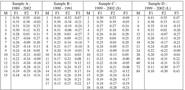
Table 1. Principal components Sample A : 1989 - 2002 Sample B : 1990 - 1991 Sample C : 1999 – 2002 (S) Sample D : 1999 – 2002 (L) M F1 F2 F3 M F1 F2 F3 M F1 F2 F3 M F1 F2 F3 1 2 3 4 5 6 7 8 9 10 11 12 13 14 15 0.34 0.33 0.31 0.30 0.28 0.27 0.26 0.25 0.24 0.22 0.22 0.21 0.20 0.19 0.18 0.55 0.38 0.24 0.12 0.03 -0.04 -0.09 -0.14 -0.18 -0.21 -0.24 -0.26 -0.28 -0.29 -0.31 -0.61 -0.02 0.23 0.32 0.31 0.27 0.20 0.13 0.05 -0.02 -0.09 -0.16 -0.21 -0.26 -0.31 1 2 3 4 5 6 7 8 9 10 11 12 13 14 15 16 17 0.41 0.39 0.34 0.31 0.28 0.25 0.23 0.21 0.20 0.18 0.17 0.16 0.15 0.15 0.14 0.13 0.13 -0.52 -0.34 -0.19 -0.06 0.03 0.09 0.14 0.17 0.19 0.21 0.22 0.23 0.24 0.25 0.26 0.26 0.27 0.67 -0.21 -0.24 -0.27 -0.27 -0.23 -0.16 -0.10 -0.03 0.03 0.08 0.12 0.15 0.17 0.19 0.21 0.22 1 2 3 4 5 6 7 8 9 10 11 12 13 14 15 16 17 18 0.30 0.29 0.27 0.27 0.26 0.25 0.25 0.24 0.23 0.23 0.22 0.22 0.21 0.20 0.20 0.19 0.18 0.18 0.52 0.39 0.27 0.18 0.10 0.04 -0.01 -0.05 -0.09 -0.13 -0.16 -0.18 -0.21 -0.23 -0.24 -0.26 -0.27 -0.28 -0.69 -0.03 0.24 0.30 0.28 0.25 0.20 0.15 0.10 0.05 -0.00 -0.05 -0.08 -0.12 -0.14 -0.17 -0.19 -0.21 1 3 6 9 12 15 18 21 24 28 48 60 72 84 0.41 0.38 0.35 0.33 0.31 0.28 0.26 0.24 0.22 0.20 0.16 0.14 0.11 0.10 0.55 0.33 0.14 0.02 -0.07 -0.13 -0.17 -0.20 -0.22 -0.25 -0.31 -0.31 -0.30 -0.30 0.47 0.12 -0.15 -0.26 -0.27 -0.25 -0.21 -0.14 -0.09 -0.01 0.22 0.32 0.37 0.43

Table 2. Variability explained by each factor (%)

Sample A : 1989 – 2002 Sample B : 1990 – 1991 Sample C : 1999 – 2002 (S) Sample D : 1999 – 2002 (L) F1 F2 F3 F4 F5 97.59 2.27 0.10 0.03 0.01 97.58 2.13 0.17 0.09 0.01 95.47 4.35 0.15 0.03 0.01 88.35 10.81 0.52 0.21 0.07