Anatomical and hemodynamic correlates of healthy human brain rhythms

(1)

(2)

ii

Université de Sherbrooke

Anatomical and hemodynamic correlates of healthy human brain rhythms

By Russell Butler

Programmes de Sciences des radiations et imagerie biomédicale

Thesis presented to the Faculty of Medicine and Health Sciences in order to obtain a Doctorate of Philosophy (Ph.D.) in Radiation Science and Biomedical Imaging from the Faculty of Medicine

and Health Sciences, Université de Sherbrooke.

Sherbrooke, Quebec, Canada June, 2019

Members of evaluation committee:

President: Martin Lepage – Médecine nucléaire et radiobiologie Director: Kevin Whittingstall - Radiologie diagnostique

Co-Director: Maxime Descoteaux – Informatique Co-Director: Pierre-Michel Bernier – Kinanthropologie Evaluator external to program: Jean-François Lepage - Pédiatrie

Evaluator external to University: Christophe Grova – Concordia University, Physics

(3)

iii

(4)

iv

“The first principle is that you must not fool yourself — and you are the easiest person to fool.”

(5)

v

Summary:

Anatomical and hemodynamic correlates of healthy human brain rhythms By

Russell Butler

Programmes de Sciences des Radiations et Imagerie Biomédicale

Thesis presented to the Faculté de médecine et des Sciences de la Santé in order to obtain a Doctorate of Philosophy (Ph.D.) in Sciences des Radiations et Imagerie Biomédicale from the

Faculté de Médecine et des Sciences de la Santé, Université de Sherbrooke, Sherbrooke, Québec, Canada, J1H 5N4

Rhythmic activity of neuronal populations in cerebral cortex can be measured non-invasively using electroencephalography (EEG). Typically, when a human subject sits quietly at rest their EEG power spectrum is dominated by a low frequency, high amplitude rhythm known as the alpha rhythm (8-16 Hz). When the subject attends to a visual stimulus, the alpha rhythm is suppressed, and a high frequency lower amplitude rhythm known as the gamma rhythm (30-90 Hz) emerges. Both alpha and gamma rhythms have been intensely studied for the past two decades, but many questions remain. This thesis will seek to address two basic questions about the alpha and gamma rhythms measured in the healthy human brain using EEG: 1) how does individual variability in alpha and gamma rhythm amplitude relate to individual variability in cortical and head anatomy, and 2) what is the relationship between healthy human brain rhythms and hemodynamic activity, ie, can fluctuations in the electrical rhythms of the brain be used to predict subsequent changes in cerebral blood flow measured using blood oxygen level dependent functional magnetic resonance imaging (BOLD FMRI)? To address question 1, both EEG and BOLD FMRI recordings have been performed in 42 healthy human subjects, and the amplitude of each subject’s EEG alpha and gamma rhythm was compared to anatomical features of their brain/head measured using T1-weighted MRI imaging. It was found that distance from active cortical tissue to EEG electrode is the best predictor of inter-individual variability in high frequency (gamma) brain rhythm – people whose brain is further from their scalp exhibit lower amplitude gamma rhythm fluctuations. To address question 2, a variety of visual stimulus patterns were designed based on the literature, to control alpha and gamma rhythms. BOLD FMRI measurements were then taken in response to the same stimuli, and it was found that the gamma rhythm does not always predict BOLD FMRI responses, in particular, stimuli that suppress neuronal synchrony while maintaining a high action potential firing rate are best at dissociating EEG gamma rhythm from BOLD FMRI. Overall, this research has improved our understanding of inter-individual variability in human brain rhythms, and the relationship of these rhythms to hemodynamic activity.

(6)

vi

Résumé

Corrélats anatomiques et hémodynamiques des rythmes sains du cerveau humain

Par Russell Butler

Programmes de Sciences des Radiations et Imagerie Biomédicale

Thèse présentée à la Faculté de Médecine et des Sciences de la Santé en vue de l’obtention du diplôme de Philosophiae Doctor (Ph.D.) en Sciences des Radiations et Imagerie Biomédicale

Faculté de médecine et des Sciences de la Santé, Université de Sherbrooke, Sherbrooke, Québec, Canada, J1H 5N4

L'activité rythmique des populations neuronales dans le cortex cérébral peut être mesurée de manière non invasive par électroencéphalographie (EEG). Généralement, lorsqu'un sujet humain est tranquillement assis au repos, son spectre de puissance EEG est dominé par un rythme de basse fréquence et de grande amplitude connu sous le nom de rythme alpha (8-16 Hz). Lorsque le sujet est exposé à un stimulus visuel, le rythme alpha est supprimé au profit d’un rythme de haute fréquence et d'amplitude inférieure, connue sous le nom de rythme gamma (30-90 Hz). Les rythmes alpha et gamma ont été beaucoup étudiés au cours des deux dernières décennies, mais de nombreuses questions demeurent. Cette thèse cherchera à répondre à deux questions fondamentales sur les rythmes alpha et gamma mesurés dans le cerveau humain sain en utilisant l'EEG : 1) comment la variabilité individuelle de l'amplitude du rythme alpha et gamma est-elle liée à la variabilité individuelle de l'anatomie corticale et de la tête, et 2) quelle est la relation entre les rythmes cérébraux sains de l’humain et l’activité hémodynamique, c’est-à-dire, peut-on utiliser les fluctuations des rythmes électriques cérébraux pour prédire les

modifications ultérieures du débit sanguin cérébral mesuré à l’aide de l’imagerie par résonance magnétique fonctionnelle en fonction du niveau d’oxygène dans le sang (BOLD FMRI) ? Pour répondre à la question 1, des enregistrements EEG et du BOLD FMRI ont été réalisés chez 42 sujets humains en bonne santé, et l’amplitude du rythme EEG alpha et gamma de chaque sujet a été comparée aux caractéristiques anatomiques de leur cerveau / tête mesurées par imagerie IRM pondérée en T1. Il a été constaté que la distance entre le tissu cortical actif et l'électrode EEG est le meilleur prédicteur de la variabilité interindividuelle du rythme cérébral à haute fréquence (gamma) - les individus dont le cerveau est le plus éloigné de leur cuir chevelu sont ceux qui présentent le moins de fluctuations d'amplitude du rythme gamma. Pour répondre à la question 2, une variété de modèles de stimuli visuels a été conçue en s’appuyant sur la

littérature afin de contrôler les rythmes alpha et gamma. Les mesures du BOLD FMRI ont ensuite été prises en réponse aux mêmes stimuli et il a été constaté que le rythme gamma ne prédisait pas toujours les réponses du BOLD FMRI, particulièrement en ce qui concerne les stimuli qui suppriment la synchronisation neuronale tout en maintenant un taux de déclenchement élevé du potentiel d'action qui sont les meilleurs pour dissocier le rythme gamma en EEG du BOLD FMRI. Globalement, ces recherches ont amélioré notre compréhension de la variabilité interindividuelle des rythmes cérébraux chez l’humain et de la relation entre ces rythmes et l’activité hémodynamique.

(7)

vii

List of Figures

Figure 1.01 – Human and Macaque monkey neurophysiological response to similar stimuli ... 1

Figure 1.02 - EEG response to the same stimulus in two healthy humans ... 2

Figure 1.03 - High resolution BOLD image ... 3

Figure 1.04 - Visual system ... 5

Figure 1.05 - Receptive fields ... 6

Figure 1.06 – Orientation columns ... 7

Figure 1.07 – Layers and hierarchy in visual cortex ... 8

Figure 1.08 – Different modalities for different scales of measurement ... 10

Figure 1.09 –Biophysics of EEG ... 11

Figure 1.10 – Gross anatomy and EEG ... 12

Figure 1.11 – Muscular contamination of high frequency EEG ... 13

Figure 1.12 – Independent Component Analysis ... 15

Figure 1.13 - Neuronal response function ... 16

Figure 1.14 - Mechanisms of gamma rhythm generation ... 17

Figure 1.15 – Feedforward and feedback in visual cortex ... 19

Figure 1.16 – Flexible relationship of gamma LFP to spiking. ... 20

Figure 1.17 – Global gamma LFP ... 21

Figure 1.18 – Broadband and narrowband gamma. ... 22

Figure 1.19 - Correlations from different studies on gamma vs structure ... 24

Figure 1.20 – Alpha Rhythm. ... 25

Figure 1.21 – Antero-posterior propagation of Alpha waves ... 26

Figure 1.22 – The cerebrovasculature ... 29

Figure 1.23 – Feedforward and feedback neurovascular signaling ... 30

Figure 1.24 – Effect of blood CO2 level on BOLD contrast ... 33

Figure 1.25 – Mechanism of BOLD ... 35

Figure 1.26 – Application of the GLM to localize brain function. ... 37

Figure 1.27 – Arterial spin labeling. ... 38

Figure 1.29 – Gamma vs BOLD coupling and uncoupling ... 41

Figure 1.30 – Spatiotemporal frequency tuning of BOLD and gamma band MEG responses compared in primary visual cortex... 42

(12)

xii

Figure 1.31 - Laminar specific alpha-BOLD and gamma-BOLD coupling ... 44

Figure 1.32 - Theory of how oscillations modulate spiking in cortex. ... 45

Figure 3.1 - Qualitative overview of EEG and BOLD responses to visual stimulation ... 57

Figure 3.2 - Quantitative analysis of EEG and BOLD responses to MC and SR ... 58

Figure 3.3 - Control CBF and CMRO2 measurements. ... 59

Figure 3.4 - Simulations of NBG as a function of input magnitude (Im) and spatial correlation (Isc) ... 62

Figure 3.5 - Spatial and temporal analysis of BOLD and NBG responses, respectively ... 63

Figure 4.1 – Three groups (n=42) EEG and BOLD results ... 76

Figure 4.2 – Consistency of inter-subject EEG amplitude across stimulus types... 78

Figure 4.3 – Distance and cancellation correlations with gamma amplitude ... 81

Figure 4.4 – Sex difference and source localization analysis ... 83

Figure 4.5 – Article 2 Supplementary 1 ... 88

Figure 4.6 – Article 2 Supplementary 2 ... 90

Figure 5.1 – Raw data and scalp segmentation procedure ... 96

Figure 5.2 – Electrode Pancake ... 98

Figure 5.3 – Electrode segmentation procedure ... 100

Figure 5.4 – UTE vs T1 gel artifacts ... 103

Figure 5.5 – Effects of spatial resolution on pancake ... 104

Figure 5.6 – Precision and reproducibility of electrode segmentation ... 106

Figure 6.1 - Effects of contrast on frequency specific EEG power ... 118

Figure 6.2 – Frequency specific EEG orientation tuning ... 119

Figure 6.3 – Replication of contrast dependent BOLD orientation tuning ... 121

Figure 6.4 – Neurophysiological basis of contrast dependent BOLD orientation tuning ... 124

Figure 6.5 – Stimuli and EEG orientation tuning analysis ... 128

(13)

xiii

List of Tables

(14)

xiv

List of Abbreviations

3D – three dimensional

AFNI – Analysis of Functional NeuroImages

AMPA - α-amino-3-hydroxy-5-methyl-4-isoxazolepropionic ANTS – Advanced Normalization Tools

ASL – Arterial Spin Labeling BET – Brain Extraction Tool

BOLD – Blood Oxygen Level Dependent CBF – Cerebral Blood Flow

CBV – Cerebral Blood Volume

CHUS – Centre Hospitalier Universitaire de Sherbrooke CMRO2 – Cerebral Metabolic Rate of Oxygen

CRT – Cathode Ray Tube CSF – Cerebral Spinal Fluid DOF – Degrees of Freedom EEG - Electroencephalography E-I – Excitatory-Inhibitory EPI – Echo Planar Imaging

ERSP – Event Related Spectral Perturbation FDR – False Discovery Rate

FMRI – Functional Magnetic Resonance Imaging FOV – Field of View

FSL – FMRIB Software Library FWHM – Full Width Half Maximum GABA – Gamma aminobutyric acid GLM – General Linear Model

HRF – Hemodynamic Response Function ICA – Independent Component Analysis LFP – Local Field Potential

LGN – Lateral Geniculate Nucleus MC – Michelson Contrast

MEG - Magnetoencephalography

MELODIC – Multivariate Exploratory Linear Optimized Decomposition into Independent Components

MNE – Minimum Norm Estimate MNI – Montreal Neurological Institute MR – Magnetic Resonance

MRI – Magnetic Resonance Imaging ms - milliseconds

MUA – Multi Unit Activity NBG – Narrow Band Gamma NHP – Non Human Primate

(15)

xv NMDA – N-methyl-D-aspartate

NRF – Neuronal Response Function NVC – Neurovascular Coupling

pCASL – pseudo Continuous Arterial Spin Labeling PVC – Polyvinyl Chloride

RF – Radio Frequency RGB – Red Green Blue ROI – Region of Interest SEM – Standard Error of Mean SENSE – Sensitivity Encoding SNR – Signal to Noise Ratio SR – Spatial Randomization std – standard deviation TE – Echo Time

TR – Repetition Time UTE – Ultra Short Echo Time V1 – Primary Visual Cortex V2 – Secondary Visual Cortex V3 – Third Visual Cortex

(16)

1

1 – Introduction

1.1 General Introduction

1.1.1 Non-invasive Brain Signals

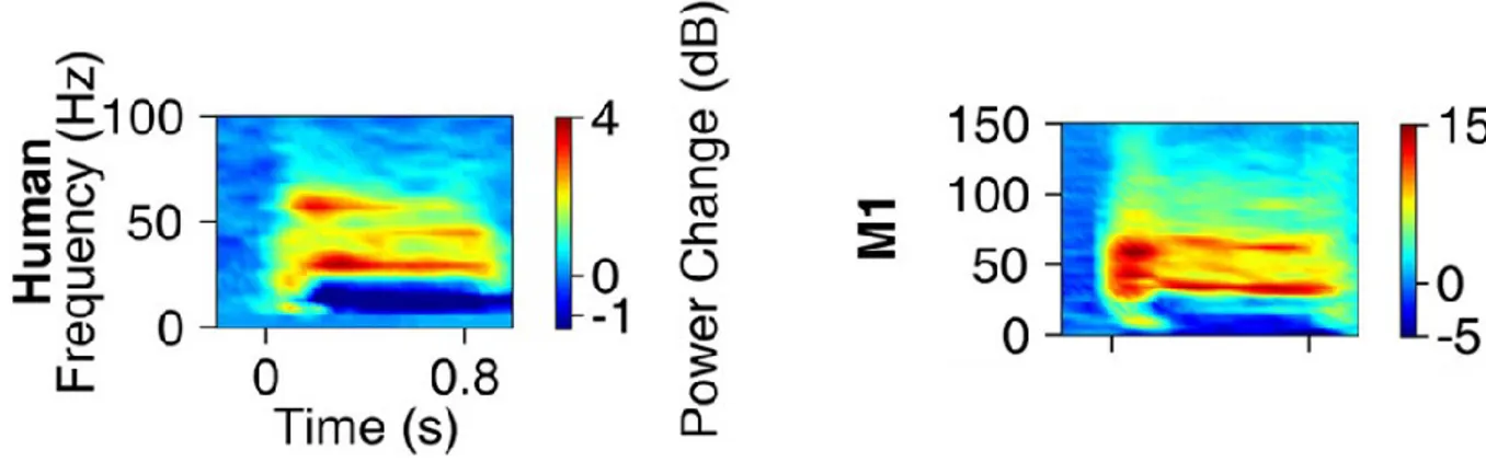
The human brain contains between 86 and 100 billion neurons, each with hundreds or thousands of connections to other neurons (Williams and Herrup 1988). Today, non-invasive measurement techniques fall far short of capturing this complexity, providing only a rudimentary viewpoint on human brain activity. The most widely used non-invasive measurement technique for direct recording of electrical human brain activity is the electroencephalogram (EEG), which uses recording sites on the scalp to measure changes in electrical potential over time. EEG provides a window into the human brain, but the signals obtained using EEG are low spatial resolution, poorly understood measures of human brain activity. Despite this, signal processing techniques reveal striking similarities between scalp EEG measured in humans and much more spatially precise local field potential (LFP) recordings using invasive microelectrodes in nonhuman primates (NHPs), giving us confidence that EEG is a reliable index of human brain activity (Figure 1.01), albeit a low spatial resolution and poorly understood one.

Figure 1.01 – Human and Macaque monkey neurophysiological response to similar stimuli

. Time-frequency decomposition from a large grating stimulus in human (left) and monkey (right). The human data was acquired using scalp EEG, the monkey data was acquired using intracranial microelectrode. Note the similarity between the two signals. Reproduced from (Murty et al. 2018)

under the Creative Commons Attribution 4.0 International License.

This thesis attempts to improve our understanding of the human EEG signal through comparing the EEG rhythms measured on the scalp with hemodynamic changes using BOLD FMRI, and anatomical differences across individuals measured using T1-weighted MRI. The hope is that through an improved understanding of how non-invasively measured EEG rhythms relate to brain

(17)

2

structure and hemodynamics, we will broaden the scope and clarify the interpretation of EEG signals measured in health and disease.

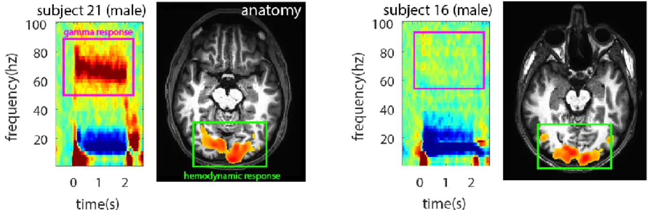
Due to the fact that EEG is measured from the surface of the scalp, 20-30 mm distant from the closest source of neuronal activity, interpreting inter-individual differences in healthy human EEG signals is difficult. Does a reduced EEG signal in one person indicate less brain activity, or simply a thicker skull or less conductive scalp? These questions, while fundamental to the understanding of EEG measurements in health and disease, remain largely unanswered (Figure 1.02).

Figure 1.02 - EEG response to the same stimulus in two healthy humans

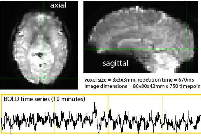
. Subject 21 (left) and subject 16 (right) from a group of healthy humans. Note how both subjects have normal anatomical structure and hemodynamic responses (green), but subject 16 lacks any discernable gamma activity while subject 21 presents a powerful gamma response.

The other major technique to be discussed is Blood Oxygen Level Dependent Functional Magnetic Resonance Imaging (BOLD FMRI), which tracks relative changes in ratio of oxyhemoglobin/deoxyhemoglobin within the venous vasculature across the entire brain, typically at a resolution of 1-3 mm (Figure 1.03). Fluctuations in the BOLD FMRI signal are thought to indirectly reflect changes in neural activity (Shmuel et al. 2004; Goense and Logothetis 2008b). BOLD FMRI has risen steadily in popularity over the past two decades, and is now the main workhorse of functional human brain imaging efforts.

The relationship between BOLD FMRI and EEG remains ill-defined and elusive. Some studies claim that BOLD FMRI is a poor index of neuronal activity (Muthukumaraswamy and Singh 2009; Swettenham et al. 2013) while others claim the opposite (Niessing et al. 2005a; Scheeringa et al. 2011). Hence, BOLD FMRI is an extremely powerful tool for probing human brain activity non-invasively, but much work remains in order to better understand the link between neuronal activity and BOLD FMRI. This thesis will investigate neurovascular coupling of brain rhythms to

(18)

3

cerebral blood flow (CBF) by comparing EEG and BOLD measurements in healthy humans to advance our understanding of the human brain in health and disease.

Figure 1.03 - High resolution BOLD image

. The time series (bottom) represents the activity within a single voxel in visual cortex over 10 minutes. Note the repetitive peaks in the time series, corresponding to visual stimulus presentation.

(19)

4

1.2.1 Visual cortex

The human brain is dominated by the cerebral cortex, a tissue with an average thickness of only 2mm, but if completely spread out, its surface would cover an area roughly 2000 cm2_{. Even more}

impressive than its size is the number of cells in the cortex, under every square millimeter reside roughly 105_{neurons, for a total of around 10}11_{neurons in the cortex alone, and the number of}

synaptic connections is orders of magnitude greater still. In short, the human cerebral cortex is the most complex structure known to man. Much of the work done on unravelling the complexity of cerebral cortex has focused on sensory areas, or parts of the cortex whose function is to process sensory stimuli from the outside world. In particular, the visual cortex is an ideal system to study cortical function, due to its large size, encompassing the entire posterior segment of the brain, and also the ease with which experimental manipulations can be designed to stimulate the visual cortex through visual stimulation of the eyes. Primate visual cortex is hierarchically organized, with low-level areas representing simple features and higher areas representing more complex aspects of the visual world. Vast inter-individual differences exist across a healthy population in visual cortex, and these differences are thought to be related to perception, cognition, and reaction time. For example, primary visual cortex (V1) size varies from 2200mm2 _{to 3400mm}2_{, and}

individual with larger visual cortex experience stronger Ponzo and Ebbinghaus illusions (Kanai and Rees 2011).

The position occupied by V1 in the visual pathway is illustrated in Figure 1.04. The main components of the pathways from the outside world to V1 are the retinae, the lateral geniculate nuclei (LGN), and V1. Roughly 1 million optic nerve fibers travel from each eye through the optic chiasm to the LGN. Half of the fibers from each eye cross over to the other side of the brain at the optic chiasm, while the other half remain uncrossed. This crossing occurs so that the left LGN receives input from the right visual field, and vice versa. The LGN is a one synapse connection from retina to V1, and is traditionally thought of as a relay station between the retina and V1.

(20)

5

Figure 1.04 - Visual system

. Diagram of the retino-geniculo-cortical pathway in a higher mammal. Brain viewed from below. Right halves of retina shown in black, projecting to left hemisphere, left halves of retina shown in white, projecting to right hemisphere. Reproduced from (“Ferrier lecture

- Functional architecture of macaque monkey visual cortex” 1977) with permission from the Royal Society U.K.

While all neurons in the visual cortex are concerned primarily with vision, they cluster together according to their physiological properties (Hubel and Wiesel 1968). In fact, visual cortical tissue can be classified not only based on morphology, but also based on functional response properties to external stimuli. V1 can be said to have two main functions – first, the input from LGN is rearranged in such a way as to make V1 cells responsive to short line segments of a specific orientation, termed ‘orientation selectivity’. Second, V1 is the first point in the retina – LGN – V1 pathway where inputs from two separate eyes synapse onto a single cell in the brain.

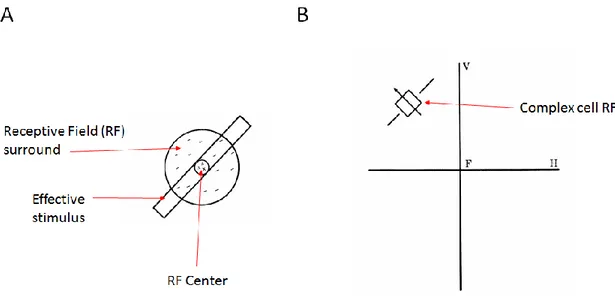
The activity of retinal, LGN, and V1 neurons can be understood using the concept of a ‘receptive field’, (Figure 1.05). In the retina, retinal ganglion cells (RGC) respond most strongly to roughly circular points of light of a certain size, and the response can be either an increase or decrease in firing rate of the RGC (KUFFLER 1953). Therefore, RGCs are sensitive to light impinging on specific clusters of photoreceptors in the retina, while light impinging on the surrounding photoreceptors has the opposite effect (Figure 2, receptive field). RGC receptive fields have circular symmetry, and hence respond equally well to lines of any orientation. In V1, due to the convergence of many RGC cell receptive fields on a single V1 neuron, we find neurons with orientation specificity,

(21)

6

meaning that the neuron possesses a rectangular receptive field, and responds to a specifically orientated stationary or moving straight line segment (Hubel and Wiesel 1968).

A moving line, swept across the V1 neuron’s rectangular receptive field at the preferred orientation, is typically more effective in evoking a discharge than a non-moving line. It was originally thought that all possible orientations are represented roughly equally in V1, but recent findings have unveiled significant orientation anisotropies, with a cardinal preponderance overall (Chapman and Bonhoeffer 1998; Li 2003), which is to say, more V1 neurons prefer vertical and horizontal orientations than oblique orientations.

Figure 1.05 - Receptive fields

. A) center-surround receptive field of typical on-center retinal ganglion cell (RGC). The diagram represents a small portion of the visual field, in primates, the diameter of the receptive field is roughly 1 visual degree or 0.3 mm on the retina. Shining light on the center region increases the firing rate of RGC, shining a light on the surround reduces the firing rate. B) Receptive field of complex cell in striate cortex. Axes represent vertical (V) and horizontal (H) meridian of visual field, crossing at gaze center F. The cell in this example responds strongly to a thin line at the appropriate orientation. Reproduced from (“Ferrier lecture - Functional

architecture of macaque monkey visual cortex” 1977) with permission from the Royal Society U.K.

The processing of visual information in V1 proceeds in a hierarchical manner, at least four distinct levels in the hierarchy are recognized, containing 4 distinct cell types 1) circularly symmetric 2) simple 3) complex and 4) hypercomplex. Circularly symmetric cells are similar to RGCs, responding strongly to circular points of light on the retina. A simple cell responds to an optimally oriented line in some narrowly defined position within the visual field. Complex cells also respond to optimally oriented lines, but are less sensitive to the exact spatial position of the line within the

(22)

7

visual field. Finally, hypercomplex cells are similar to complex cells, but are also sensitive to the length of the optimally oriented line stimulus.

The V1 processing hierarchy is understood in terms of a feed forward network with each higher layer receiving inputs from many cells in the layer below. For example, a simple cell receives inputs from many circularly symmetric cells (which form a line), while a complex cell receives inputs from many simple cells (sensitive to orientation at specific regions of visual field). Orientation specificity occurs in specific clusters of V1, termed ‘columns’, and cells within columns are always sensitive to the same line orientation (Hubel and Wiesel 1974) (Figure 3). Indeed, inserting an electrode tangentially into V1 and tracking orientation selectivity as the electrode is pushed further into V1 reveals an orderly shift in orientation preference depending on the tangential position of the electrode. Inserting an electrode perpendicularly to the cortical surface, however, reveals the same pattern of orientation selectivity throughout the entire depth of cortex. A 180° shift in orientation takes place over roughly 1 mm tangential distance across the cortex, and the width of a cortical column is roughly 20-50um (Hubel and Wiesel 1968) (Figure 1.06).

Figure 1.06 – Orientation columns

. A) Orientation columns in cat cerebral cortex, color coded according to preferred orientation. Reproduced from (Obermayer and Blasdel 1993) with

permission from The Journal of Neuroscience 1993. B) Orientation tuning as a function of electrode

track distance for tangentially inserted electrode in visual cortex. Note how the orientation preference measured by the electrode changes as a function of tangential distance. Reproduced

from (“Ferrier lecture - Functional architecture of macaque monkey visual cortex” 1977) with permission from the Royal Society U.K.

(23)

8

Morphologically, V1 is typically divided into six layers on the basis of histology data, with every layer receiving a unique pattern of inputs and emitting a distinct set of axonal projections to other layers and brain structures (Self et al. 2013) (Figure 1.07). More superficial layers are those closer to the pial surface, while deeper layers are closer to the white matter. Layer 4 is in the middle. While role of the different layers in cortical processing is still poorly understood, it is known that V1 receives feedforward input from LGN that terminates primarily in layer 4. There are horizontal connections between the different cortical columns at all layers but terminating predominantly in upper layer 4 and the superficial layers, and there are feedback connections from higher order visual areas, which avoid layer 4 and terminate primarily in layers 1 and 5. When examining neuronal responses time locked to visual input, the shortest latencies always occur in input layers 4 and 6, with longer latencies in layer 5 and the superficial layers (Self et al. 2013). The receptive field tuning properties mentioned earlier reflect what is known as feedforward processing, but additional modulations occur in V1, evoked by the horizontal and feedback connections. The second visual area to receive visual input is called V2, with a response latency only 10 ms greater than that of V1 (45 ms vs 35 ms) (Lamme, Supèr, et al. 1998). The role of these higher order visual areas (V3, and V4 in addition to V2) in modulating activity within V1 can be tested by inactivating the higher order areas while measuring from V1. It was shown that stimuli presented to both center and surround of a V1 cell evoked a larger response when V2 was inactivated (Sandell and Schiller 1982), indicating that feedback connections from V2 play a role in the suppressing effect of a V1 receptive field’s surround, thereby sculpting receptive field properties. Feedback on V1 from even higher areas such as MT also exist. Cooling of area MT reduces response strengths in V1 and reduces the inhibitory effects of moving surround stimuli (Lamme, Supèr, et al. 1998).

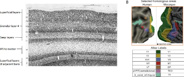
Figure 1.07 – Layers and hierarchy in visual cortex

. Cross section through monkey striate cortex showing conventional layering designations. Reproduced from (“Ferrier lecture - Functional

(24)

9

B) Selected human-macaque homologous visual areas displayed on flat cortical maps. Black sites indicate injection site of retrograde tracer to map feedback connections. Reproduced from

(Michalareas et al. 2016) with permission from Elsevier.

1.2.2 Physiology of EEG

Neuronal activity in the cortical layers gives rise to transmembrane currents that can be measured in the extracellular medium. The synaptic transmembrane current is the major source of the extracellular signal, but other sources, including Na+_{and Ca}2+_{spikes can also shape the}

extracellular field (Buzsáki et al. 2012a). The current sources and sinks form dipoles or higher-order n-poles (Nunez and Srinivasan 2006a). All currents in the brain superimpose to yield an electric potential (Ve) at any given point in space, with respect to a reference potential. Ve can be

measured at high temporal resolution using extracellularly placed electrodes, and these measurements can be used to interpret neuronal activity.

Ve when measured from the scalp is known as EEG, when measured from the cortical surface

ECOG, and when measured from intracranial electrodes, LFP (Figure 1.08). Synaptic activity is the most important source of extracellular current flow for distal measurements such as ECOG and EEG. This is due to the fact that currents from many extracellular compartments must overlap in time to induce a measurable signal at distance, and this overlap is more easily achieved by slower events such as synaptic currents, than for sharper events such as action potentials which are less likely to overlap temporally (Nunez and Srinivasan 2006a).

Neurons in the layers of cerebral cortex can be modeled as dipolar or higher order current sources. This is due to the spatial arrangement of their dendrites and soma, which form a tree-like structure with an electrically conducting interior surrounded by an insulating membrane. This membrane is studded with thousands of synapses that allow the transfer of Na+ or Ca2+ ions into the cell, increasing the membrane potential and giving rise to an extracellular current sink. This inflow of current is balanced by a passive return current mediated by ionic pumps in the cell membrane (which is metabolically expensive), giving rise to an extracellular source forming a dipole or higher order n-pole, depending on the relative locations of the sink and source. The contribution of a dipole to Ve is proportional to 1/r2, due to the first order cancellation of the two

(25)

10

Figure 1.08 – Different modalities for different scales of measurement

. A) Simultaneous recorded LFP traces from superficial and deep layers of motor cortex in anaesthetized cat as well as intracellular trace from layer 5 neuron. Note the alternation of hyperpolarization and depolarization of the layer 5 neuron and corresponding changes in LFP. B) 5 seconds of slow waves recorded by scalp EEG, LFP, and depth electrode in different cortical areas. Reproduced from

(Buzsáki et al. 2012b) with permission from Springer Nature.

In a cytoarchitecturally regular structure such as mammalian cerebral cortex, the synaptic activity of pyramidal cells make the largest contribution to Ve (Figure 1.09). This is due to several factors

1) pyramidal cells are the most populous cell type 2) pyramidal cells have long and thick apical dendrites that generate strong dipoles along the somatodendritic axis which gives rise to an open field 3) pyramidal cells are aligned in an orderly fashion perpendicular to the cortical surface, allowing the activity from multiple cells to sum in Ve. The macro-scale curvature of mammalian

cortex is also important for Ve, areas such as a sulcus where apical dendrites from one cortical

bank oppose apical dendrites on the adjacent bank results in effective cancellation at the level of Ve. The orientation of the dipole axis with respect to the measurement location is also important

(Figure 1.09).

In addition to the geometry of cortex, temporal properties of neuronal activity are also important in determining Ve. In general, lower frequency membrane currents are associated to higher

amplitude Ve, indeed, there exists a 1/f scaling for amplitude of Ve, where f is temporal frequency

of the LFP signal (Miller et al. 2009a). This scaling is attributed to low-pass frequency filtering property of dendrites which affects frequencies as low as 10 Hz for the pyramidal neurons used in modeling studies (Lindén et al. 2010). Other factors such as network mechanisms also play a role in the 1/f scaling of Ve amplitude. The low frequency nature of the Ve power spectrum can

(26)

11

neurons can contribute for a shorter time window, while for longer time windows, more neurons can contribute to Ve, increasing the amplitude of Ve at lower frequencies (Buzsáki et al. 2012b).

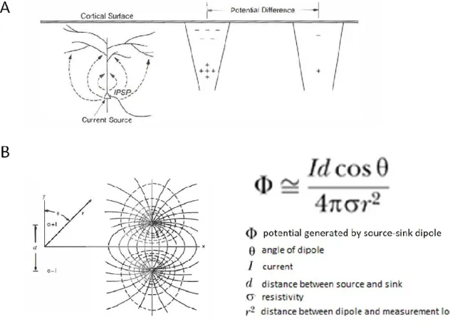
Figure 1.09 –Biophysics of EEG

. A) Synaptic action at membrane surfaces caused by inhibitory and excitatory postsynaptic potentials (IPSP, EPSP) creates balanced local current sources and sinks. B) The current dipole consists of source and sink separated by distance d. Current lines (solid) and equipotential boundary (dashed) for dipole in infinite saltwater tank. The equation to the right provides a reasonable approximation for potential generated by source-sink configuration in (A) for the case of a homogenous isotropic volume. Large distances from measurement location to dipole results in widely spaced current lines and lower current density.

Reproduced from (Nunez and Srinivasan 2006a) with permission from Oxford University Press.

Ve, when measured from the scalp using EEG, is highly dependent on volume conduction. The

intervening tissues from dipole source to scalp electrode can be modeled as layered media distinctly separated into two or more sub-regions having different conductivities σ1, σ2, σ3, etc. The skull, scalp, gray matter, white matter, blood, and cerebrospinal fluid (CSF) all have different conductivities, and the skull itself is a 3-layered structure with the middle layer substantially more conductive than the outer layers. Due to the fact that electrical current follows the path of least

(27)

12

resistance in an inhomogenous medium, the interpretation of Ve at the scalp is complicated

relative to Ve measured directly within the brain. In general however, if the brain to skull

conductivity ratio is high, Ve measured outside the head using surface electrodes will be lower

(Nunez and Srinivasan 2006a). Weaker scalp signals can therefore be interpreted as less conductive head tissue. Loss in signal amplitude can also occur when distributed sources are active simultaneously, such as the case across a large swathe of cortical V1 in response to a full field visual stimulus. While EEG is less sensitive to source orientation than magnetoencephalography (MEG) (Lutkenhoner 1998), cancellation between simultaneously active sources still occurs due to superposition of electric fields. This reduces the signal to noise ratio of sources, resulting in a scalp measurement (EEG) that is sensitive to the geometry of the underlying cortical folds (Irimia et al. 2012a). Source localization seeks to account for all these effects (distance from dipole, volume conduction, cortical folding) through use of the forward model (Figure 1.10). (Gramfort et al. 2010).

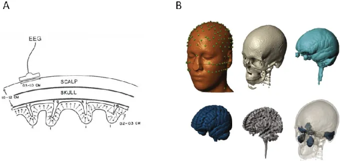
Figure 1.10 – Gross anatomy and EEG

. A) Cortical sources modeled as dipole layers in cortical fissures and sulci, EEG is sensitive to gyral crowns (region a-b, d-e, g-h, j-k). Reproduced from

(Nunez and Srinivasan 2006a) with permission from Oxford University Press. B) Segmentation of

human head into six different tissue types: scalp (with electrodes), skull, cerebro-spinal fluid, gray matter, white matter, and air cavitites. Reproduced from (Huang et al. 2016) under the Creative

(28)

13

1.2.3 EEG confounds and data processing

Due to the 1/f nature of Ve, high frequency (40 Hz+) neural activity is weak at large distances, such

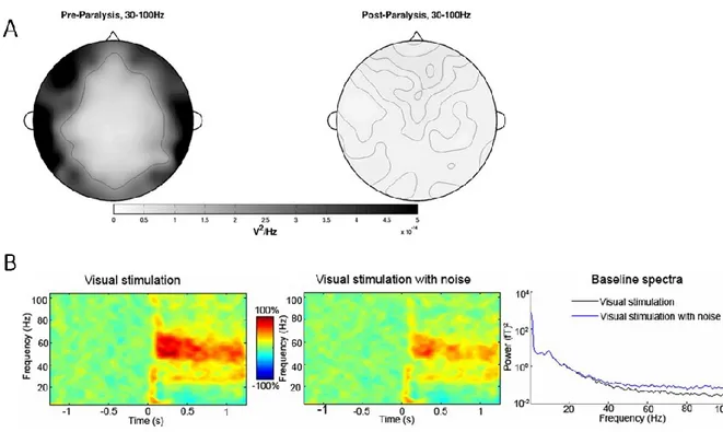
as in the case of an EEG recording. Unfortunately, the spectral band of muscle activity is also in this range (20-300 Hz), and experiments using paralysis of head and neck muscles reveal that muscle artifacts account for over 90% of the high frequency content of resting state EEG activity (Figure 1.11) (Whitham et al. 2007). The high frequency content of EEG became of interest due to work showing stimulation of brainstem reticular formation leads to suppression of slow EEG rhythms and emergence of low-voltage fast waves (Moruzzi and Magoun 1949). Further work revealed more specific activations such as the 50 Hz oscillation in human V1 during visual stimulation (Chatrian et al. 1960) and influential work suggesting these frequencies play an important signal processing role in the brain (Gray et al. 1990). However, the diversity of the muscular system in the face and neck ensures that without proper signal processing techniques many muscles will contaminate EEG including the masseter muscle, involved in chewing peaks in amplitude at 50-60 Hz, the frontalis, involved in brow control at 30-40 Hz, and a 40-80 Hz bandwidth for temporal muscles (O’Donnell et al. 1974).

Figure 1.11 – Muscular contamination of high frequency EEG

. A) Scalp topography pre and post paralysis of neck and face muscles illustrating strong contribution of EMG to spectral power in scalp electrodes during eyes-closed task. Reproduced from (Whitham et al. 2007) with

(29)

14

participant to a grating stimulus, white noise has been added to the channel prior to computation resulting in clear attenuation of the high frequency response. Baseline spectra shows high frequency MEG is easily affected by noise. Reproduced from (Muthukumaraswamy 2013) under

the Creative Commons Attribution License.

Muscular (and other) contamination necessitates advanced signal processing to separate neuronal signals of interest from physiological artifacts in the EEG signal. The most popular method is Independent Component Analysis or ICA, a technique pioneered by Terrence Sejnowski (Jung et al. 1997) used to separate independent sources linearly mixed in several sensors. ICA when applied to EEG involves several pre-processing steps in order to obtain more physiologically plausible components. First, the data is high pass filtered to remove frequencies below 1 Hz (Winkler et al. 2015). This is done in order to remove large portions of variance from the data which are not related to the neural signal of interest, as well as increase independence between sources by removing the slowly changing trends. After high pass filtering, the data is whitened, decorrelating the EEG channels. ICA then works in the following way:

We start by assuming we measure a mixture (Y) of two signals (S): Y1 = a11S1 + a12S2

Y2 = a21S1 + a22S2

We would like to obtain S1 as a function of the mixtures Y1 and Y2. Therefore, we would like to

construct the matrix b such that S1 = b11Y1 + b12Y2.

The fundamental assumption that allows ICA to work is that S1 and S2 are independent of one

another. Based on this assumption, the values of b can be found through gradient descent optimization with kurtosis as the cost function. Kurtosis is used as the cost function due to the fact that a signal with a high kurtosis distribution is less Gaussian than a signal with a low kurtosis distribution. By the Central Limit Theorem, the distribution of the sum of two independent signals is more Gaussian than either signal alone, therefore by deriving values for b that maximize the non-Gaussianity (kurtosis) of S1 and S2, ICA is able to extract independent components from a

(30)

15

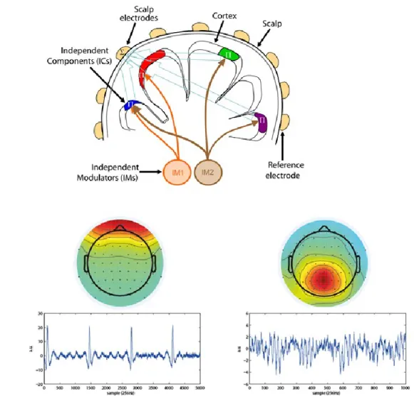
Figure 1.12 – Independent Component Analysis

. A) Outline of problem for ICA. Independent neuronal modulators cause spatially distributed activity in cortex, measured with an array of scalp electrodes, each electrode records a linear combination of Independent modulator signal.

Reproduced from (Onton and Makeig 2009) (Open Access). B) Two independent components from

a healthy human EEG subject recording, scalp maps (top) and time series reveal physiologically plausible weight maps and temporal activity.

ICA decomposes channel-based EEG signals into independent components, in the ideal case, each component represents a specific type of physiological artifact or neuronal source. In practice, ICA maps 64 electrodes (assuming a 64 channel EEG cap) to 64 maximally independent sources, ranking the sources in terms of their variance explained in the raw signal. Using these sources, the researcher must then select which components to retain and which to subtract from the raw signal, a time consuming and subjective procedure. One method to automatically select

(31)

16

components is using the stimulus design. If the stimulus design for the experiment is known, ICA components can be selected/rejected based on their correlation to external stimuli, for instance, a ‘neuronal response function’ (NRF) can be defined based on established time-frequency signature of visual cortex activity to a stimulus and used to rank ICA components based on their NRF similarity (Figure 1.13). All EEG analysis presented in this work relies on the extraction of 3-5 components per subject based on the NRF.

Figure 1.13 - Neuronal response function

. Created by averaging narrow band ICA components across all subjects (n=24), the neuronal response function (NRF) characterizes frequency specific modulation for a given stimulus. The NRF can be used to rank ICA components according to their correlation.

Using ICA, it is possible to extract signals from EEG recordings that are similar in spectral content to those obtained from LFP recordings in macaque monkeys exposed to the same stimulus (Fries et al. 2008a; Murty et al. 2018). This is a promising result, indicating that non-invasive studies using EEG can answer many of the same questions that invasive electrophysiology in experimental animals seek to address.

EEG also has its limitations however. For example, studies using ECOG (Bartoli et al. 2019), LFP (Ray and Maunsell 2010), and MEG (Kupers et al. 2015) have all reported distinct high frequency activity of a broadband nature likely due to neuronal spiking in higher (100+ Hz) frequencies, while broadband high frequency activity of neuronal origin has yet to be commonly observed in the EEG signal (but see (Onton and Makeig 2009)). This is in large part due to the increased muscular contamination of EEG signals relative to LFP, ECOG, or even MEG (Muthukumaraswamy 2013), and more advanced signal processing algorithms (other than ICA) or better recording equipment

(32)

17

to reduce scalp-electrode impedance are clearly needed to extract these sensitive high frequency fluctuations from the EEG signal.

1.2.4 Gamma rhythm

One of the most commonly observed and widely debated rhythms in the EEG signal is the gamma rhythm or gamma oscillation. Cortical gamma oscillations (30-90 Hz) are associated to increases in focused attention and external sensory drive. Gamma oscillations are generated by synchronous activity of fast-spiking inhibitory interneurons, producing synchrony across a neural ensemble through limiting the time window for effective excitation (Figure 1.14). Networks of fast-spiking inhibitory cells provide large, synchronous inhibitory postsynaptic potentials to local excitatory neurons (Hasenstaub et al. 2005), which is sufficient to induce oscillations in the gamma range (30-90 Hz) that are regulated by fast excitatory feedback from pyramidal cell neurons (Whittington et al. 1997). This can be seen from in-vivo cortical recordings showing that sensory-evoked gamma oscillations in the LFP are phase-locked to the firing of excitatory pyramidal cells, indicating entrainment of excitatory neurons to rhythmic inhibitory activity (Gray and Singer 1989). Cortical gamma oscillations appear to be a fundamental mode of neuronal activity. They are ubiquitous across phyla from insects (Stopfer et al. 1997) to humans (Fries et al. 2008a), across cortical regions from motor (Murthy and Fetz 1992) to parietal (Pesaran et al. 2002) to visual cortex (Fries et al. 2007), and across a range of tasks including working memory (Pesaran et al. 2002) and attentional selection (Fries 2001).

Figure 1.14 - Mechanisms of gamma rhythm generation

. Simplified representation of laminar structure of feedforward pathway in V1. Thalamic inputs project to E and I cells in layer 4, which excite more superficial layers 2 and 3. In both layers, there are inhibitory (I) and excitatory (E)

(33)

18

neurons with reciprocal projections. The pyramidal-interneuron gamma (PING) mechanism proposes a synchronous volley of excitation from feedforward pathway is necessary to elicit synchronous volley from I cells. The frequency of the oscillation is determined by the time of recovery of E cells from reciprocal I cell inhibition. Reproduced from (Tiesinga and Sejnowski 2009)

with permission from Elsevier.

Multiple hypotheses about the function of cortical gamma rhythms exist. 1) The binding by synchronization hypothesis (Singer and Gray 1995) states that neurons forming an assembly to perform a distinct function are bound together by synchronization of their action potentials, facilitated by refinement of intra and inter-areal connections through experience. The gamma rhythm, which synchronizes pyramidal cell firing across large areas, could be the mechanism by which V1 groups features of the visual world possibly allowing for faster object recognition. 2) Others believe that the gamma cycle serves to convert the excitatory input to pyramidal cells into a temporal code, whereby the amplitude of excitation is recoded in the time of occurrence of output spikes relative to the gamma cycle, with stronger inputs leading to earlier responses. Gamma oscillations in V1 would thus convert amplitude to phase, and pyramidal cells discharging early in the gamma cycle would silence those receiving less excitation, creating a winner-take-all situation in response to V1 input enabling fast processing and readout of stimuli (Fries et al. 2007). For either of these hypotheses to be accurate, ie, for the gamma cycle to function as a temporal reference signal in the brain, the phase and frequency of gamma bursts must be conserved over time (autocoherence).

This was found not to be the case, in fact, LFP recordings in Old World monkeys showed chance level autocoherence in gamma bursting activity within V1, being statistically indistinguishable from filtered noise (Burns et al. 2011). This lack of temporal structure provides evidence for a third hypothesis, that gamma activity is simply filtered noise output of recurrent interactions in V1 that serve no additional function (Kang et al. 2010). According to this theory, the resonant frequency or peak gamma frequency of excitatory-inhibitory interactions in V1 depends on the amount of cortical feedback, for example, in the case of large visual stimuli, the resonant frequency would shift downwards due to increased feedback over a wider cortical area.

Recent work from multiple labs indicates a role for gamma in indexing feedforward activity from the visual outside world, to higher order visual processing (Figure 1.15) (Bastos et al. 2014; van Kerkoerle et al. 2014; Michalareas et al. 2016). MEG experiments using granger causality to investigate directed influences between V1 and higher cortical areas, combined with homologous connectivity maps derived from tract tracing in macaque show that influences along feedforward projections predominate in the gamma band (Michalareas et al. 2016). Another study using

(34)

19

laminar electrodes revealed gamma waves are initiated in input layer 4 of V1, and propagate to deep and superficial layers (van Kerkoerle et al. 2014).

Figure 1.15 – Feedforward and feedback in visual cortex

. A) Schematic representation of Granger causality between layers for gamma and alpha rhythms. Thicker arrows indicate stronger Granger causality. Reproduced from (van Kerkoerle et al. 2014) with permission from National

Academy of Sciences (Copywrite 2014). B) Coherence and Granger causality influence spectra

between higher order area DP and V1. Feedforward between areas occurs in the gamma band, feedback in the alpha band. Reproduced from (Bastos et al. 2014) with permission from Elsevier. Whatever the function of gamma, it is clearly dissociable from multi-unit spiking activity (MUA) in stimulus response properties in V1, and understanding the spatial extent of gamma and its relationship to MUA is critical for interpreting this signal. This can be addressed by simultaneously recording both gamma LFP and spiking using microelectrode arrays implanted in macaque V1. One such experiment revealed that the spatial extent of gamma and its relationship to spiking activity was stimulus dependent (Jia et al. 2011). Small gratings, and those masked with noise induced a broadband increase in spectral power, this broadband signal was similarly tuned to spiking activity and had a limited spatial coherence. Larger gratings however elicited a distinct gamma rhythm with a pronounced spectral peak at 40 Hz, coherent across large areas of V1 (up to and exceeding 10mm) (Figure 1.16).

(35)

20

Figure 1.16 – Flexible relationship of gamma LFP to spiking.

A) Normalized firing rate (dashed) and gamma power (solid) as a function of stimulus size. Large gratings also resulted in spatially correlated orientation tuning in the gamma range. B) Correlation across all sites between spiking and gamma (solid) and between gamma and gamma (dashed) as a function of stimulus size. Note how inter-site gamma is more correlated for larger gratings. Reproduced from (Jia et al. 2011) with

permission from The Journal of Neuroscience 2011.

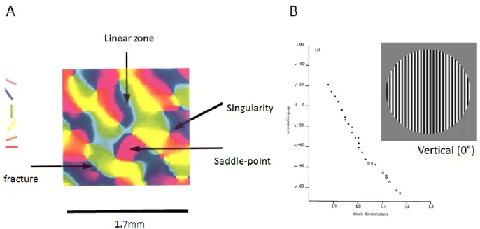
Fascinatingly, averaging LFP signals across recordings sites several millimeters apart revealed a global tuning preference in the gamma range of V1 (Figure 1.17). Termed ‘global gamma’, this signal had strong spatial and temporal frequency tuning preferences, responding most strongly from 2.5 cycles/degree gratings drifting at 2 cycles/second. Orientation tuning preferences of global gamma were also stimulus dependent and distinct from local MUA (Figure 1.17), gratings with low noise levels dissociated MUA orientation tuning preferences from global gamma, while more randomized gratings suppressed global gamma, and orientation tuning more closely matched that of local MUA (Zhou et al. 2008; Jia et al. 2011). The orientation tuning preference of global gamma was also adaptable. Adaptation, or the decreased response to the same stimulus over multiple repetitions, is well known to reduce the responsivity of cortical neurons whose preferences match the adapter, but have little effect on cells with offset preferences (Kohn 2007). This provides evidence towards the hypothesis that global gamma magnifies a bias in the neuronal representation of orientation. The global nature of the adaptive gamma rhythm suggests an additional spatially extensive mechanism that coordinates or drives inhibitory network activity.

(36)

21

The mechanism that gives rise to global gamma could be feedback connections extending over large areas also thought to contribute to the surround suppression recruited by large stimuli (Angelucci and Bressloff 2006). Another possible mechanism is the emergence of global gamma through coordination of local generators by long-range lateral connections, or gap-junction coupling among inhibitory neurons (Tiesinga and Sejnowski 2009).

One thing is certain, that any mechanism contributing to emergence of global gamma must be more effective for some stimuli than others. The fact that global gamma emerges strongly in the presence of non-randomized gratings and is suppressed by spatial randomization of the grating (Zhou et al. 2008; Jia et al. 2011) suggests a larger role for the local generator mechanism rather than feedback connection mechanism, and the fact that global gamma is stronger for large rather than small gratings (Jia et al. 2013) may simply be due to a larger cortical area being activated (rather than increased feedback due to larger stimulus).

Figure 1.17 – Global gamma LFP

. A) The global gamma LFP. LFP averaged across 31 sites in a single implant, large gratings (top) induced spatially extensive rhythm evident through averaging while small gratings did not (bottom). B) MUA and gamma orientation tuning distributions. MUA tuning followed a uniform distribution while gamma tuning clustered around a specific orientation. Reproduced with permission from (Jia et al. 2011) with permission from The Journal

of Neuroscience 2011.

It is clear from the above studies that LFP recordings in the gamma range have two distinct components with very different stimulus response properties (Figure 1.18). One is a narrow band,

(37)

22

spatially coherent rhythm with very specific and spatially extensive (global) stimulus tuning preference that is distinct from MUA. The other is a broadband signal sharing stimulus tuning preferences with MUA such as local orientation preference. These two components have been clearly dissociated in a recent ECOG and LFP studies (Ray and Maunsell 2011a; Hermes, Miller, et al. 2014; Bartoli et al. 2019), and, based on the spectral profile of narrow-band and broadband gamma, EEG is clearly more sensitive to narrow-band gamma (Fries et al. 2008a; Scheeringa et al. 2011; Perry et al. 2013). Therefore, it seems reasonable to assume that gamma activity measured from the scalp is predominantly sensitive to the global gamma LFP mentioned in (Jia et al. 2011), rather than the broadband component. This is supported by the fact that, due to its distance from the source, EEG is sensitive primarily to synchronized synaptic activity with the possibility to sum at a distance, which would be the case for a spatially extensive rhythm such as global gamma and less so for broadband gamma (but see (Kupers et al. 2015) where specific denoising techniques reveal broadband gamma using MEG). This has several implications for studies using EEG to investigate gamma activity.

Figure 1.18 – Broadband and narrowband gamma.

A) Mean group ECOG task selectivity spectrogram for gratings vs image categories. Note the sustained narrowband gamma for Gratings and more broadband gamma for Categories. B) Mean group amplitude responses for narrow and broadband gamma during early and late time windows. Reproduced from (Bartoli et al. 2019) with

(38)

23

First, EEG visual cortex gamma can only be dissociated from background muscular artifacts when a strong, sustained stimulus is used, due to the fact that 1) 90% of electrical activity in the gamma range is generated by head/neck muscles (Whitham et al. 2007), 2) micro-saccades (and possibly other micro-movements) are time locked to visual stimulus presentation (Keren et al. 2010) but can be avoided by removing the first 500 ms of each trial and 3) the poor SNR of EEG necessitates a great number of trials (usually 100+ per stimulus type), so obtaining quality gamma band signals using EEG requires both a clean baseline and stimulus induced period. If a strong, sustained visual stimulus is used, however, gamma band activity can serve as a sensitive and remarkably consistent marker of subject specific neuronal activity (Muthukumaraswamy et al. 2010a; Gaetz et al. 2012). The second implication is, due to the fact that EEG gamma is difficult to disentangle from confounding factors such as muscular artifacts, gamma signals acquired in the resting state from clinical populations should be interpreted with caution. For example, multiple studies have reported increased baseline/resting state gamma band amplitude in autism relative to healthy controls (Orekhova et al. 2007; van Diessen et al. 2015; Ethridge et al. 2017), but other studies using strong, sustained visual stimuli show reduced responses in autism vs control (Sun et al. 2012; Simon and Wallace 2016a). This suggests that studies reporting increased gamma power in baseline gamma may be confounded by muscular artifacts. Other studies investigating peak frequency rather than amplitude have reported increased peak frequency in autism vs healthy controls (Dickinson et al. 2015a), which may be a more robust measure of gamma measured through EEG, as peak frequency can be estimated robustly even in the presence of noise artifacts (Magazzini et al. 2016).

Finally, despite its limitations the presence of a sustained narrowband gamma response in response to visual gratings in scalp EEG has generated much excitement, and is perhaps the most sensitive direct measure of neuronal activity that can be acquired in humans non-invasively. Consequently, there is great interest in exploring possible anatomical/neurochemical correlates of scalp gamma, in particular GABA concentration (Muthukumaraswamy et al. 2009) (but see (Cousijn et al. 2014a)), GABA receptor density (Kujala et al. 2015a), cortical surface area (Schwarzkopf et al. 2012), cortical thickness (Gaetz et al. 2012) and sex (van Pelt et al. 2018) have all been linked to gamma peak frequency/amplitude (Figure 1.19).

(39)

24

Figure 1.19 - Correlations from different studies on gamma vs structure

. A) Gamma peak frequency vs V1 surface area. Reproduced from (Schwarzkopf et al. 2012) with permission from

The Journal of Neuroscience 2012. B) Gamma peak frequency vs GABA concentrations in V1. Reproduced from (Muthukumaraswamy et al. 2009) with permission from the National Academy of Science (Copywrite 2012). C) Gamma peak frequency vs V1 surface area. Reproduced from (Robson et al. 2015a) with permission from John Wiley and Sons. D) Gamma peak frequency vs

GABA concentrations in V1. Note how some studies show significant correlations while others show no correlations for the exact same metrics. Reproduced from (Cousijn et al. 2014b) with

(40)

25

1.2.5 Alpha Rhythm

The alpha rhythm (Figure 1.20) (7-13 Hz) is the longest studied brain rhythm, discovered nearly 100 years ago by Hans Berger in the mid 1920’s with the invention of EEG (Berger 1929), but its physiology remains poorly understood. Alpha oscillations are prominent in EEG during relaxed wakefulness, and thought to be fundamental for top-down cognitive processes (von Stein and Sarnthein 2000; Ito et al. 2005) such as working memory, attention (Saalmann et al. 2012), perception (Samaha and Postle 2015), and feedback inhibition (Jensen and Mazaheri 2010).

Figure 1.20 – Alpha Rhythm.

Time series taken from posterior EEG electrode over occipital lobe during the eyes closed resting state condition. Note the prominent oscillation at 1.5 seconds, each wave lasts approximately 100 ms for a temporal frequency of ~10 Hz.

Two hypotheses about the generation of alpha in cortex exist 1) cortical alpha is driven by thalamic pacemaker (Hughes et al. 2011; Vijayan and Kopell 2012) such as pulvinar or LGN and 2) alpha arises predominantly through intra-cortical interactions, via infragranular layers driven by layer 5 pyramidal cells (Silva et al. 1991; van Kerkoerle et al. 2014; Mejias et al. 2016).

Recent invasive results in humans (Halgren, Devinsky, et al. 2017) supports the second viewpoint, that cortical alpha arises predominantly through intra-cortical interactions and thalamus plays a more limited role. This study employed both ECOG and depth electrodes to study spontaneous alpha activity in humans, showing that alpha oscillations propagate as travelling waves from anterosuperior cortex towards posteroinferior areas (Figure 1.21) and similar results have been found in macaques (Nagasaka et al. 2011). To determine if the thalamus was involved in coordination of these traveling alpha wave, simultaneous depth recordings were also performed in the cortex and pulvinar nucleus of the thalamus of human patients. Surprisingly, alpha was much more prevalent in the cortex than thalamus of these depth recordings, and the peak frequency could sometimes differ from cortex to thalamus (Halgren, Devinsky, et al. 2017), suggesting a very limited role for the thalamus in generating cortical alpha. However, thalamocortical coherence spectra often exhibited robust alpha peaks, indicating functional coupling between alpha in thalamus and cortex. To examine whether cortical alpha was driven by

(41)

26

thalamic firing or vice versa, broadband gamma power, which provides an index for MUA (as discussed earlier) was extracted from depth electrodes in both thalamus and cortex. Thalamic alpha was rarely synchronous with broadband gamma power and instead predominantly synchronous with cortical gamma, indicating that thalamic alpha was driven by cortical firing, and not the other way around (Halgren, Devinsky, et al. 2017).

Figure 1.21 – Antero-posterior propagation of Alpha waves

. ECOG recording during period of high alpha activity reveals an antero-posterior direction for the propagation of alpha waves, visible through the increased phase offset in the more posterior channels relative to anterior channels. Reproduced from (Halgren, Ulbert, et al. 2017) under the CCBY-NC-ND 4.0 license

(Non-Commerical Creative Commons).

The layered structure of the cortex is thought to be important in generation of the alpha rhythm, this can be investigated using laminar electrodes to record current source density (CSD) and MUA across gray matter layers. The CSD is important because it allows for measurement of a volume-conduction free measure of local transmembrane currents surrounding the laminar probe (Nicholson and Freeman 1975), isolating activity in the different cortical layers. This analysis has revealed that alpha band power is strongest in the superficial layers 1-3 (Halgren, Devinsky, et al. 2017). Furthermore, CSD recordings have shown a succession of sinks starting in layers 1,2 and 5 and propagating towards layer 4 throughout the alpha cycle (van Kerkoerle et al. 2014). MUA in layers 1, 2, and 5 also precedes MUA in layer 4 for all frequencies between 5 and 15 Hz, indicating that alpha waves are initiated in layers 1, 2 and 5 and propagate towards layer 4, opposite the direction of gamma waves.

In addition to the propagation from superficial/deep layers 1, 2 and 5 to layer 4, there is also a phase lag from V1 to V4 in the alpha range (Castelo-Branco et al. 1998; von Stein et al. 2000; Ito

(42)

27

et al. 2005). This implies that alpha oscillations start in higher order cortical areas such as V4 and then propagate to lower areas such as V1. This can be demonstrated using microstimulation in V1 and downstream V4 while simultaneously recording from both sites (van Kerkoerle et al. 2014). Microstimulation in V1 produced gamma oscillations in V4, but had little effect on V4 alpha power. Microstimulation in V4, however led to increases in V1 alpha power and a suppression of gamma power, providing further evidence that alpha waves travel in the feedback direction. The V4 microstimulation effects were also stimulus dependent: a task involving segregation of figure from background revealed that V4 microstimulation led to maximal increases in V1 alpha when the receptive field of the neurons in the stimulated area fell on the background of the stimulus. Thus, V1 neurons are particularly susceptible to V4 feedback effects when their receptive field falls on the background of an image, reinforcing the role of alpha in attention and feedback inhibition. Alternatively, recent evidence supports a more important role for subcortical nuclei in the generation of scalp alpha, showing that electrophysiological activity in deep brain structures can be measured directly using scalp EEG (Seeber et al. 2019).

Inter-individual variability in the alpha rhythm remains an area of active research. Age-related changes in alpha have been reported, with decreases in peak frequency (Knyazeva et al. 2018) over the lifespan, reduced connectivity of inter-hemispheric alpha sources associated to mild cognitive impairment (MCI) (Babiloni et al. 2018), and larger event-related alpha desynchronization in the motor cortex associated to cortical thinning in healthy aging (Provencher et al. 2016a). Differences in white matter connectivity or anisotropy (Valdés-Hernández et al. 2010) are also though to play a role in determining inter-individual alpha, due to the fact that alpha reflects inter-areal directed influences from higher order cortical areas onto V1 (Michalareas et al. 2016) (but see (Renauld et al. 2016)).