A New Approach to the Evaluation of Non
Markovian Stochastic Petri Nets
Serge Haddad1, Lynda Mokdad1, and Patrice Moreaux2
1 LAMSADE, UMR CNRS 7024, Université Paris Dauphine Place du Maréchal de Lattre de Tassigny
75775 PARIS Cedex 16, FRANCE {haddad, mokdad}@lamsade.dauphine.fr
2 LISTIC, ESIA-Université de Savoie Domaine universitaire d’Annecy le Vieux BP 806, 74016 ANNECY Cedex, FRANCE
Abstract. In this work, we address the problem of transient and steady-state analysis of a stochastic Petri net which includes non Markovian dis-tributions with a finite support but without any additional constraint. Rather than computing an approximate distribution of the model (as done in previous methods), we develop an exact analysis of an approx-imate model. The design of this method leads to a uniform handling of the computation of the transient and steady state behaviour of the model. This method is an adaptation of a former one developed by the same authors for general stochastic processes (which was shown to be more robust than alternative techniques). Using Petri nets as the mod-elling formalism enables us to express the behaviour of the approximate process by tensorial expressions. Such a representation yields significant savings w.r.t. time and space complexity.
1
Introduction
Non Markovian process analysis The transient and steady-state analysis of Markovian discrete event systems is now well-established with numerous tools at the disposal of the modellers. The main open issue is the reduction of the space complexity induced by this analysis. However in a realistic system, the distri-bution of the occurrence (or the duration) of some events cannot be described by an exponential law (e.g., the triggering of a time-out). Theoretically any “reasonable” distribution is approximated by a phase-type distribution enabling again a Markovian analysis [1]. Unfortunately the continuous time Markov chain (CTMC) associated with this approximation is so huge that it forbids its anal-ysis (indeed even its construction). Such a phenomenon often occurs when the non exponential distribution has a finite support i.e., when the whole probability mass is included in a finite subset of IR+ (non null Dirac, uniform, etc.); then a good phase-type approximation requires too much stages for a close approxima-tion.
Hence the research has focused on alternative methods. In the case of a single realization of a non Markovian distribution at any time, successful methods have been proposed [2] both for the transient and steady state analysis, especially in the Stochastic Petri Net (SPN) modelling framework. Let us cite, for instance, the method of supplementary variables [3,4] or the method of the subordinated Markov chains [5].
The general case (i.e., simultaneous multiple realizations of such distribu-tions) is more intricate. The method of supplementary variables is still theo-retically applicable but the required space and the computation time limit its use to very small examples. An alternative approach is described for non null Dirac distributions (i.e., “deterministic” durations) in [6]. The stochastic process, which is a General State space Markov Process (GSMP) is observed at periodic moments of time ({h∆ | h ∈ IN}) and this new process is expressed by a system of integro-differential equations and solved numerically. The steady-state dis-tributions of these processes are identical and, with another computation, one obtains the transient distribution of the original process from some transient distribution of the transformed process. This method has been implemented in the DSPNexpress tool [7] (but currently for only two concurrent “determinis-tic” events with same duration). By imposing conditions on the simultaneous occurrences of concurrent activities, other authors have also designed efficient algorithms [8,9,10,11,12] (see section 6 for more details).
Our previous contribution In [13] we have proposed a different approach to deal with multiple concurrent events with finite support distributions. Moreover, in contrast with other works, our solution does not require specific synchronization between these events such as non overlapped or nested events. The main idea is to define an approximate model on which we perform an exact analysis. To this end, given a time interval (say ∆) we describe the behaviour of the stochastic model by two components: a CTMC and a discrete time Markov chain (DTMC). During an interval (h∆, (h + 1)∆) the behaviour is driven by the CTMC which corresponds to Markovian events occurring in (h∆, (h + 1)∆). Non Markovian activities are taken into account at h∆ instants only: the corresponding untimed probabilistic changes of state are processed according to a DTMC.
In the approximate process, the Markovian events are in fact exactly mod-elled since the set {h∆ | h ∈ IN} has a null measure. The approximation comes from non Markovian events: the distribution of a non Markovian event is ap-proximated by a discrete random variable expressing the number of points h∆ that must be reached before its occurrence. Thus the residual number of points to be met is included in the state of the approximate process. At any moment h∆, the current residual numbers are decreased and the corresponding events occur when their residues are null.
The approximate process may be analysed either in transient mode or in steady-state. The transient analysis is done by successively computing the state distribution at the instants ∆, 2∆, . . . , h∆, . . . applying a transient analysis of the CTMC during an interval ∆ (via the uniformization technique [14]) followed by a “step” of the DTMC. In order to smooth the effect of the discretization, we
average the distribution upon the last interval with a variant of uniformization. Since the asymptotic behaviour of the process depends on the relative position w.r.t. the points h∆, the approximate process does not admit a steady-state dis-tribution but it is asymptotically periodic. Hence, for the steady-state analysis, one computes the steady-state distribution at the instants h∆ and then starting from this distribution, one again averages the steady-state distribution upon an interval.
Our current contribution Standard benchmarks (like M/D/S/K queue) have shown that the implementation of our method is at least as efficient as tools like DSPNexpress-NG [15]. Furthermore it is robust, i.e., it still provides good approximations under extreme situations like loaded heavy queues unlike other tools. However, the space complexity is the main limitation of our method since a state includes its logical part and the delays of each enabled non Markovian event. In order to tackle this problem, we start with a high-level description given by a stochastic Petri net with general distributions. Then we define its semantics by specifying the associated stochastic process. Afterwards, we introduce an approximate stochastic process for the stochastic Petri net whose behaviour is structured as described above.
Thus we give tensorial expressions for the infinitesimal generator of the con-tinuous part of our process and for the probability transition matrix of its discrete part. More precisely, these matrices are decomposed into blocks and each block is associated with a tensorial expression. Such a structure is a consequence of the representation of the state space. Indeed rather than (over-)approximating the state space by a cartesian product (as done in the original tensorial methods), we approximate it by a finite union of such products yielding a significant space reduction. A similar approach has been successfully experimented with in [16] for SPNs with phase-type distributions.
Here, we face an additional difficulty. Inside an interval, the delay of each enabled general transitions is non null whereas it can be null at the bounds of the interval. Thus the state space of the discrete part of the process is an extension of the one of the continuous part. Furthermore, the block decomposition must be refined. Indeed inside the interval, states are grouped w.r.t the general enabled transitions. At the bounds, states are grouped w.r.t both the general enabled transitions and the fireable ones (i.e., with null delay). Thus the alternation between the continuous part and the discrete part requires a tricky expansion of the probability vector. Hopefully, the complexity of this operation is negligible w.r.t. the other parts of the computation.
The experimentations are still in progress and their results will be provided in a forthcoming LISTIC technical report. Nevertheless we will detail here some key features of the implementation.
Organization of the paper In section 2 we recall the principle of our approach for a general stochastic process. Then we present the approximate process of a stochastic Petri net in section 3. Afterwards we develop in section 4 the tensorial expressions of the matrices defining the behaviour of this approximate process.
We give information about our implementation in section 5. In section 6, we show that all the previous methods handle particular cases of the systems that we are able to analyse. Finally we conclude and we give indications on future developments of our work.
2
The approximate method
2.1 Principle
Semantics of the approximate process As mentioned in the introduction, we define an approximate model (say Y(∆)) of the initial model (say X), on which we perform an exact analysis. The main idea is to choose a time interval ∆ and to restrict in Y(∆) the non Markovian events to only occur at times t
h = h∆.
We then study in an exact way the evolution of the stochastic process Y(∆) in each interval (th, th+1) and during the state changes at time th . We stress that
the starting times of the active non Markovian events are in no way related. We obtain such a model Y(∆) from a general model with non Markovian finite
Fig. 1: Time decomposition
support distributions as follows. The distribution of every non Markovian event is approximated by a discrete time distribution lying on points h∆. Let us note that although ∆ seems to be the approximation parameter, the appropriate parameter is the maximum number of points used to express the distribution. Moreover this indicator is the key factor for the complexity of our analysis.
In the approximate process, the Markovian events occur during the intervals (h∆, (h + 1)∆). Non Markovian events always occur in {h∆ | h ∈ IN}. Let us describe how they are scheduled. When a non Markovian event is enabled in an interval (h∆, (h + 1)∆) due to the occurrence of a Markovian event, then its approximate distribution is interpreted as the number of points k∆ that must be met before its occurrence. Here we can choose whether we count the next point (i.e., an under-evaluation of the approximated distribution) or not (i.e., an overestimation of the approximated distribution). The impact of this choice will be discussed later. Thus the residual number of points to be met is included in the state of Y(∆). At any moment h∆, the current residual numbers correspond-ing to non Markovian events are decreased. If some residues are null then the corresponding (non Markovian) events occur with possibly some probabilistic choice in case of conflicts. The occurrence of these events may enable new non Markovian events. Such events are handled similarly except that the next point
is always counted since now it corresponds to a complete interval. If we denote by t−
h (t+h) the “time” before (after) the state change in th, the process Y(∆) is
defined by two components:
– the subordinated process in (th, th+1) associated with states at t+h records
only exponential events. It is then a CTMC defined by its generator Q; – the state changes at th are defined by a stochastic matrix
P[i, j] = Pr(Y(∆)(h∆+) = j | Y(∆)(h∆−) = i).
Thus the Markov Regenerative Process (MRGP) Y(∆) is fully defined by its initial probability vector π(0) and the matrices P, Q (figure 1). These three components depend on ∆ since the state space includes the residual number of instants per activated event. We stress however that, even if non Markovian events occur at h∆, all kinds of concurrency are allowed between the activities of the system, contrary to previous methods.
Furthermore, it is important to note that in the approximate process, the Markovian events are in fact exactly modelled since the set {h∆ | h ∈ IN} has a null measure. The only approximation comes from non Markovian events: their approximate distribution is interpreted as the number of points k∆ that must be met before their occurrence.
This approximate process may be analysed either in transient mode or in steady-state. The proposed analysis is an adaptation of the classical Markovian renewal theory methods.
Transient analysis The transient analysis is performed by successively comput-ing the state distribution at the instants ∆, 2∆, . . . applycomput-ing a transient analysis of the CTMC during an interval ∆ (via the uniformization technique [14]) fol-lowed by a “step” of one of the DTMC. In order to smooth the effect of the discretization, we average the distribution on the last interval (with a variant of the uniformization).
Let π(h∆+) be the probability vector of the process Y(∆) at time h∆ after the discrete time change, and πX the probability vector of the initial model. We
have:
π(h∆+) = π((h − 1)∆+)eQ∆P = π(0)(eQ∆P)h
Since we want to smooth the discretization effect, we define the approximate value π(a)(h∆) of π
X(h∆) as the averaged value of the probabilities of the states
of Y(∆) in [t h, th+1]: π(a)(h∆) = 1 ∆ Z (h+1)∆ h∆ π(τ )dτ = 1 ∆π(0)(e Q∆P)h Z ∆ 0 eQτdτ (1) Finally, we are in general interested by performance measures defined on the states of the system, and not on the states of the stochastic process Y(∆). Hence, all components of π(a)(t) corresponding to a given state of the original system (i.e., when neglecting the residual numbers) are summed up to compute perfor-mance measures.
Steady-state analysis Since the distribution depends on the relative position w.r.t. the points h∆, the approximate process does not admit a steady-state dis-tribution but it is asymptotically periodic, with period ∆. We first compute the (approximate) steady-state distribution at times h∆: π(∆) def= lim
h→∞π(h∆+).
This steady-state distribution is computed by a transient analysis stopped when the distribution is stabilised. Since Y(∆) is asymptotically periodic with ∆ as period, we average the steady-state distributions on an interval [0, ∆]. Then the approximate steady-state distribution is given by:
π(a)= 1 ∆π ∆ Z ∆ 0 eQτdτ (2)
As in the transient case, all components of π(a) corresponding to a given state of the system are summed up to compute performance indices.
2.2 Numerical considerations
Formulae (1) and (2) for transient and steady-state probabilities involve vector-matrix products with possibly very large matrices, either eQ∆ or I(∆)= R∆
0 eQτdτ . Moreover, it is well-known (and reported as the “fill in” phenomenon) that, although Q is generally very sparse, eQτ is not sparse at all. Since these matrices are only required through vector-matrix products, the usual approach [17] is to never compute these matrices explicitly but to compute directly the vector-matrix products avoiding the fill in phenomenon. The products of a vector by an exponential matrix are based on the series expansion of the exponential matrix (uniformization) and numerical summation until a required precision level is reached. This is the method that we have implemented.
When we need eQτ we follow the uniformization approach [18]. If A
u =
I + 1uQ is the uniformised matrix of Q with rate u > maxi{|qii|}, we have
eQτ =X k≥0 e−uτ(uτ ) k k! (Au) k (3) For the transient solution (1), π(0) (eQ∆P)h is computed iteratively. During
the algorithm only one current vector V indexed on the state space is required (two for the intermediate computations) and for each step we apply the vector-matrix product method to V · eQ∆P. The computation of I(∆) =R∆
0 eQτdτ is based on (3). By definition, I(∆) =P k≥0 hR∆ 0 e−ut (ut) k k! dt i (Au)k
An elementary derivation with integration by parts and summation gives: I(∆)= 1 u X k≥0 " 1 − e−u∆ h=kX h=0 (u∆)h h! # (Au)k (4)
As for eQ∆, we only need I(∆) through products 1
∆ · V · I(∆). We compute
in [19] for steady-state solution of Deterministic Stochastic Petri Nets (DSPN) but restricted to one deterministic event at any given time.
Steady-state solution is obtained in a similar way, steps V(m+1)= V(m)eQ∆P being computed until convergence.
Algorithm 2.1 : Computing the approximate probability distribution (time horizon τ )
// ² is the required precision
// n0 is the initial value of n, the subdivision factor
// inc is the additive term applied to n at each step of the iteration begin n ← n0 compute π(L)n (τ ) and π(H)n (τ ) V ← (π(L)n (τ ) + π(H)n (τ ))/2 repeat n ← n + inc oldV ← V oldπ(L)n (τ ) ← πn(L)(τ ) oldπ(H)n (τ ) ← πn(H)(τ ) compute π(L)n (τ ) and π(H)n (τ ) d(L)n ← 1/ k πn(L)(τ ) − oldπn(L)(τ ) k d(H)n ← 1/k πn(H)(τ ) − oldπ(H)n (τ ) k V ←³d(L)n π(L)n (τ ) + d(H)n πn(H)(τ ) ´ /³d(L)n + d(H)n ´ d ←k V − oldV k until d ≤ ² // V is the approximation end
Choosing an approximate probability vector Recall that our goal is to give an approximate probability vector π(a)either at time τ or in steady-state for models with finite support distributions. The parameter of the approximation is given by n leading to the interval length ∆ = 1/n.
The computation of the approximate π(a)(τ ) is given in Algorithm 2.1 for the transient case with a given time horizon τ . The main idea is to compute successive approximation vectors until a given level ² of precision is reached. At each step we increase the precision of the approximation by decreasing the size ∆ of the elementary interval. In the algorithm, we use the L1 norm k π1− π2k=
P
i|π1[i] − π2[i]| to compare two probability distributions π1and π2and the precision of the approximation is given by the distance between successive vectors.
The special feature of the algorithm lies in the definition of our approximate vector (V). Recall (see section 2.1), that for a given n (hence ∆) we can choose between two approximations depending whether we count or not the next k∆ to be met in the value returned by the discrete random variable corresponding the distribution of a non Markovian event. This gives us two approximate vectors at time h∆ denoted by πn(L)(τ ) and πn(H)(τ ). We observed during our
exper-iments that the sequences (π(L)n (τ ))n∈{n0+k·inc} and (π
(H)
n (τ ))n∈{n0+k·inc} are
both convergent but that k πn(L)(τ ) − πn(H)(τ ) kn∈{n0+k·inc}does not necessarily
converge to 0. Moreover, several comparisons have shown that depending on the parameters, one of the two sequences converges faster than the other and that the corresponding limit is closer to the exact distribution (when available) than the other one. These behaviours have led us to define the approximate distribu-tion for n as a weighed sum of π(L)n (τ ) and π(H)n (τ ) based on their respective
convergence rate as given in the algorithm. Note that, as usual with efficient iterative methods, we are not able to estimate analytically the convergence rate. The steady-state approximate distribution algorithm is defined similarly ex-cept that the successive approximations are computed with the method explained in the steady-state analysis paragraph.
Note that we compute iteratively the sums (1) and (2) so that we only store two probability vectors during computation and no (full) exponential matrix.
3
Application to stochastic Petri nets
3.1 Presentation of stochastic Petri nets
Syntax A stochastic Petri net is a Petri net enhanced by distributions associ-ated with transitions. In the following definition, we distinguish two kinds of transitions depending on whether their distribution is exponential or general. Definition 1. A (marked) stochastic Petri net (SPN) N = (P, T, P re, P ost, µ, Φ, w, m0) is defined by:
– P , a finite set of places
– T = TX ] TG with P ∩ T = ∅, a finite set of transitions, disjoint union of
exponential transitions TX and general transitions TG sets
– P re (resp. P ost), the backward (resp. forward) incidence matrix from P × T to IN
– µ, a function from TX to IR+∗, the strictly positive rate of exponential
tran-sitions
– Φ, a function from TG to the set of finite support distributions defining the
distributions of the general transitions
– w, a function from TG to IR+∗, the weight of the general transitions
– m0, a integer vector of INP the initial marking
– dmax(t) = dInf (x | Φ(t)(x) = 1)e denotes the integer least upper bound of the support of Φ(t) (i.e., the range of a random variable with distribution Φ(t)).
– Let m be a marking, En(m) = {t | m ≥ P re(t)} denotes the set of enabled transitions. EnX(m) = En(m) ∩ T
X(resp. EnG(m) = En(m) ∩ TG) denotes
the set of enabled exponential (resp. general) transitions. – TG= {t1, . . . , tng}.
We assume that ∀t ∈ TG, Φ(t)(0) = 0, meaning that a general transition
cannot be immediately fired. This also excludes the possibility of immediate transitions. This restriction is introduced only for readability purposes. In a forthcoming technical report, we will indicate how we handle this case which requires more complicated computation also encountered with discrete time SPN [20,21,11].
Semantics We briefly sketch the dynamic behaviour of the stochastic process associated with an SPN. In fact, we give two equivalent descriptions. The former is a standard one whereas the latter takes into account the properties of the exponential distribution.
• First description At some time τ , a tangible state of the stochastic process is given by a marking m and a vector d of (residual) non null delays over En(m). The process lets time elapse until τ + dmin where dmin = Inf (d(t)) decrementing the delays. Let F ired be the subset of transitions such that the corresponding delay is now null. The process performs a probabilistic choice be-tween these transitions whose distribution is defined according to their weights (for this semantics, we associate also weights with exponential transitions). Let t be the selected transition, an intermediate state is reached with marking m0 = m − P re(t) + P ost(t). If (F ired \ {t}) ∩ En(m0) 6= ∅, the process
per-forms again a choice between these transitions and fires the selected transition. This iterative step ends when all the transitions in F ired have been selected or disabled at least once. Given m0 the reached marking, a new tangible state is
now obtained by choosing a delay for every t ∈ En(m0) such that either t was not
enabled in one of the previous markings or t was fired. This probabilistic choice is done according to Φ(t) or to the exponential distribution of parameter µ(t) (depending on the type of the transition). Note that delaying these choices after F ired has been exhausted does not modify the semantics due to our assumption about Φ(t)(0).
• Second description At some time τ , a tangible state of the stochastic process is given by a marking m and a vector d of (residual) non null delays over EnG(m).
The process “computes” probabilities of some events related an hypothetical de-lay (say also d(t)) for every t ∈ EnX(m) chosen according to the exponential
distribution of parameter µ(t) and an hypothetical induced dmin = Inf (d(t) | t ∈ En(m)). These (mutually exclusive) events are: dmin is associated with a single exponential transition t or dmin is associated with a set of general transitions, F ired. The other cases have a null probability to occur. We note
dminG = Inf (d(t) | t ∈ EnG(m)) Thus the process randomly selects one of
these cases according to these probabilities and acts as follows:
– The hypothetical dmin is associated with a single exponential transition t. The process selects a delay dcur for firing t according to a conditional distribution obtained from the exponential one by requiring that dcur < dminG. Then the process lets time elapse until τ + dcur and the delays
of general transitions are decremented. Afterwards t is fired and for every transition t0∈ EnG(m0) \ EnG(m) a new delay is chosen according to Φ(t0).
– dmin = dminGis associated with a set of general transitions denoted F ired.
The process lets time elapse until τ + dminG decrementing the delays. Then
the process performs a probabilistic choice between the transitions of F ired w.r.t. their weights. Let t be the selected transition, an intermediate state is reached with marking m0 = m−P re(t)+P ost(t). If (F ired\{t})∩En(m0) 6=
∅, the process performs again a choice between these transitions and fires the selected transition. This iterative step ends when all the transitions in F ired have been selected or disabled at least once. Given m0the reached marking, a
new tangible state is now obtained by choosing a delay for every t ∈ EnG(m0)
such that either t was disabled in one of the previous markings or t was fired. This probabilistic choice is done according to Φ(t).
Discussion When defining semantics for SPNs one must fix three policies: the service policy, the choice policy and the memory policy. Here in both cases we have chosen the simplest policies. However most of the other choices do not yield significant additional difficulties w.r.t. the application of our generic method. Let us detail our policies. First, we have chosen the single server policy meaning that whatever is the enabling degree of an enabled transition t we consider a single instance of firing for t. Second, we have chosen the race policy meaning that the selection of the next transition to be fired is performed according to shortest residual delay: this is the standard assumption. In order to select transitions with equal delays, we perform a probabilistic choice defined by weights. Last, we have chosen the enabling memory meaning that the delay associated with a transition is kept until the firing or the disabling of the transition. Finally, the firing of a transition t is considered as atomic meaning that we do not look at the intermediate marking obtained after consuming the tokens specified by P re(t) in order to determine which transitions are still enabled.
3.2 An approximate stochastic process for SPNs
The approximate process we propose behaves as the generic process of section 2. It is parameterized by n and ∆ = 1/n where the greater is n the better is the approximation.
First we compute for t ∈ TG, Φn(t) an approximate discrete distribution of
Definition 2. Let Φ(t) be a finite support distribution with integer l.u.b. dmax(t) such that Φ(t)(0) = 0. Then the distribution Φn(t) is defined by the
random variable X:
– whose range is defined by rangen(t) = {1, 2, . . . , n·dmax(t)−1, n·dmax(t)},
– and P rob(X = i) = Φ(t)(i/n) − Φ(t)((i − 1)/n).
The semantics of the approximate process is close to the second description of the semantics of the SPN. However, here the time is divided in intervals of length ∆ and the firings of a general transition may only occur at some h∆. At a time τ ∈ [h∆, (h + 1)∆), a tangible state of the approximate process is defined by a marking m and and a vector d of (residual) non null delays over EnG(m).
The residual delay d(t) ∈ {1, 2, . . . , n · dmax(t) − 1, n · dmax(t)} and is now interpreted as the number of intervals to elapse before the firing of t.
The process “computes” probabilities of some events related to an hypothetical delay (say also d(t)) for every t ∈ EnX(m) chosen according to the exponential
distribution of parameter µ(t) and an hypothetical induced dmin = Inf (d(t) | t ∈ EnX(m)). These (mutually exclusive) events are: dmin < (k + 1)∆ − τ and
dmin is associated with a single exponential transition t or dmin > (k +1)∆−τ . The other cases have a null probability to occur. Thus the process randomly selects one of these cases according to these probabilities and acts as follows:
– The hypothetical dmin < (k+1)∆−τ is associated with a single exponential transition t. The process selects a delay dcur for firing t according to a conditional distribution obtained from the exponential one by requiring that dcur < (k + 1)∆ − τ . Then the process lets time elapse until τ + dcur and the delays of general transitions are unchanged as the process lies in the same interval. Afterwards t is fired and for every transition t0 ∈ EnG(m0)\EnG(m)
a new delay is chosen according to Φn(t0).
– dmin > (k+1)∆−τ . The process lets time elapse until (k+1)∆ decrementing by one unit the delays. Let F ired be the subset of transitions of EnG(m) with
a null delay. Then the process performs an probabilistic choice between the transitions of F ired defined by their weight. Let t be the selected transition, an intermediate state is reached with marking m0 = m − P re(t) + P ost(t).
If (F ired \ {t}) ∩ En(m0) 6= ∅, the process performs again a choice between
these transitions and fires the selected transition. This iterative step ends when all the transitions in F ired have been selected or disabled at least once. Given m0 the reached marking, a new tangible state is now obtained
by choosing a delay for every t ∈ EnG(m0) such that either t was disabled
in one of the previous markings or t was fired. This probabilistic choice is done according to Φn(t).
At this stage, it should be clear that this approximate process is a special case of the process we have described in section 2. During an interval (h∆, (h + 1)∆), only the Markovian transitions fire whereas at time points h∆, only the general transitions fire. It remains to define the state space of this stochastic process and the associated matrices P and Q.
4
From a SPN to the tensorial expressions of its
approximate process
4.1 The state space associated with the matrix Q
As usual with the tensorial based methods, we build an over-approximation of the state space. However here, this over-approximation is reduced since we represent the state space as a finite union of cartesian products of sets instead of a single cartesian product.
First, one builds the reachability graph of the untimed version of the SPN. It is well-known that all the reachable markings of the SPN are also reachable in this setting. Let us denote the set of reachable markings M , the second step consists in partitioning M w.r.t. the equivalence relation m ≡ m0iff EnG(m) = EnG(m0).
Thus M = M (T E1) ] . . . ] M (T Ee) with T Ei ⊆ TG and M (T Ei) = {m ∈ M |
EnG(m) = T E i}.
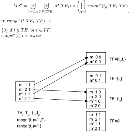
According to section 3.2, M S the set of tangible states may be decomposed as follows: M S = ] i=1..e M (T Ei) × Ãn g Y g=1 rangen(tg, T Ei) ! where rangen(t, T E i) is: – {0} if t /∈ T Ei, – rangen(t) otherwise
In this expression, we have associated an artificial delay (0) with each disabled general transition. This does not change the size of the state space and makes easier the design of the tensorial expressions.
4.2 Tensorial expression of Q
Let us recall that the matrix Q expresses the behaviour of the SPN inside an interval (h∆, (h + 1)∆). Thus a state change is only due to the firing of an expo-nential transition. As usual with tensorial methods for continuous time Markov chains, we represent Q = R − Diag(R · 1). The matrix R includes only the rates of state changes whereas the matrix Diag(R · 1) accumulates the rates of each row and s it on the diagonal coefficient. Generally the latter matrix is computed by a matrix-vector multiplication with the tensorial expression of R and then stored as a (diagonal) vector. Thus we focus on the tensorial expression of R. More precisely, due to the representation of the state space, R is a block matrix where each block has a tensorial expression. We denote Ri,j the block
corresponding to the state changes from M (T Ei) ×
¡Qng g=1rangen(tg, T Ei) ¢ to M (T Ej) × ¡Qng g=1rangen(tg, T Ej) ¢
We first give its expression and then we detail each component. Ri,j= " X t∈TX µ(t)R0 i,j(t) # OÃOng g=1 R0 i,j(tg) !
For t ∈ TX, the matrix R0i,j(t) is a binary matrix (i.e., with 0’s and 1’s) only
depending on the reachability relation between markings: the presence of a 1 for row m and column m0 witnesses the fact that m−→ mt 0.
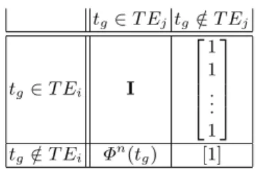
For tg ∈ TG, the matrix R0i,j(tg) expresses what happens to the delay of tg
when an exponential transition is fired. An important observation is that this matrix does not depend on the fired transition. Indeed it only depends on the enabling of tg in M (T Ei) and M (T Ej), i.e., whether tg ∈ T Ei and tg ∈ T Ej.
If tg belongs to both the subsets, the delay is unchanged (yielding the identity
matrix I). If tg does not belong to T Ej, the delay is reset to 0. Finally, if tg
belongs to T Ej and does not belong to T Eithe delay is randomly selected w.r.t.
the distribution Φn(t g) (see table 1). tg∈ T Ej tg∈ T E/ j tg ∈ T Ei I 1 1 .. . 1 tg ∈ T E/ i Φn(tg) [1]
Table 1: Structure of matrices R0 i,j(tg)
Due to the previous observation, rather than computing the matrices the matrix R0
i,j(t) for every t ∈ TX, it is more efficient to compute their weighted
sum: RXi,j= X t∈TX µ(t)R0 i,j(t)
Furthermore, this computation can be performed on the fly when building the reachability graph of the net.
4.3 The state space associated with the matrix P
The matrix P expresses the instantaneous changes at instants h∆. Such a change consists in decrementing the delays of the enabled general transitions followed by successive firings of general transitions with null delays (see section 3.2).
First, observe that the delay of a general enabled transition t during the intermediate stages may be either 0 (when ready to fire) or any value in rangen(t)
(when newly enabled). Thus the state space needs to be expanded to include null delays for enabled transitions. Furthermore, the matrix decomposition into blocks needs to be refined in order to obtain a tensorial expression. Indeed the decomposition associated with Q was based on the set of the enabled general transitions. Here a block will correspond to a pair (T Ei, T F ) where T F ⊆ T Ei
represents the enabled transitions with null delay. We call such a transition a fireable transition.
Thus M S0 the set of vanishing states may be decomposed as follows: M S0 = ] i=1..e ] T F ⊆T Ei M (T Ei) × Ãn g Y g=1 rangen(t g, T Ei, T F ) ! where rangen(t, T E i, T F ) is: – {0} if t /∈ T Ei or t ∈ T F , – rangen(t) otherwise
Fig. 2: Expanding the state vector while decrementing the delay
During the computations, we will expand the current probability vector then we will multiply it by P and afterwards contract it. Figure 2 illustrates the expan-sion of a block M (T Ei)× ¡Qng g=1rangen(tg, T Ei) ¢ into blocksUT F ⊆T E iM (T Ei) סQng g=1rangen(tg, T Ei, T F ) ¢
. We have represented inside the boxes the indices of the vectors (and not their contents). In fact, we perform simultaneously the expansion and the decrementation of the delay. The copy of contents are repre-sented by the arrows. The contraction is not reprerepre-sented as it is straightforward to design. It consists in copying the contents of the block associated with T F = ∅ to the original block.
4.4 Tensorial expression of P
In order to describe the matrix P we adopt a top-down approach. First, P = DE·(Pone)ng·C where DE corresponds to the delay decrementation phase with
vector. We do not detail these matrices since, in the implementation, they are not stored. Rather the effect of their multiplication is coded by two algorithms whose time complexities are linear w.r.t. the size of the probability vector. The matrix Ponerepresents the change due to the firing of one fireable general transition in a
state or no change if there is no such transition. Depending on the state reached at the instant h∆ and of the choice of the transitions, a sequence with variable length of general transitions may be fired. However due to our assumption about the distributions, this length is bounded by ng. Thus our expression is sound.
Let us detail Pone. We denote Pone(i, T F, j, T F0) the block corresponding to
the state changes from M (T Ei) ×
¡Qng g=1rangen(tg, T Ei, T F ) ¢ to M (T Ej) × ¡Qng g=1rangen(tg, T Ej, T F0) ¢ .
If T F = ∅ then Pone(i, ∅, i, ∅) = I and for every (j, T F0) 6= (i, ∅)
Pone(i, ∅, j, T F0) = 0.
Assume now that T F 6= ∅ then Ponecorresponds to a probabilistic choice of
a transition in T F and its firing. Thus we write: Pone(i, T F, j, T F0) = X t∈T F w(t) P t0∈T F w(t0) Ponet (i, T F, j, T F0)
Similarly to the case of Q, Pone
t (i, T F, j, T F0) can be expressed as a tensorial
product: Ponet (i, T F, j, T F0) = PM(t, i, j) OÃOng g=1 PG(tg, t, i, T F, j, T F0) ! . The binary matrix PM(t, i, j) only depends on the reachability relation be-tween markings: the presence of a 1 for row m and column m0 witnesses the fact
that m −→ mt 0. These matrices can be computed on the fly when building the
reachability graph of the untimed net.
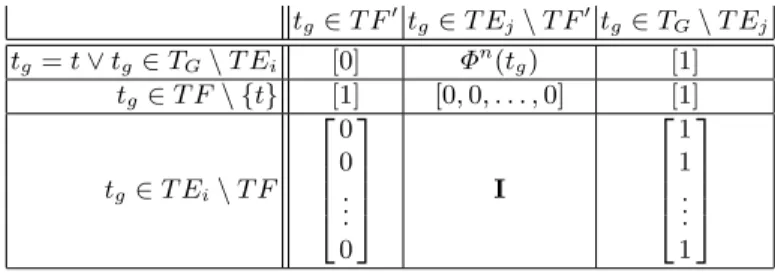
For tg ∈ TG, the matrix PG(tg, t, i, T F, j, T F0) expresses what happens to
the delay of tg when t is fired. Its structure is described in table 2. The only
possibility for tgto be fireable is that it was still fireable and not fired (second row
of first column). If tgis enabled but not fireable, then it was still in this situation
with the same delay or was disabled and then the delay is chosen according to its distribution (see the second column). If, after the firing of t, tg is disabled
then its delay is reset (see the third column of the table).
5
Implementation details
Our implementation is coded in the Python language [22] completed with the Numerical package [23] for better linear algebra computations and the sparse package [24] for efficient handling of sparse matrices. All our computations were done on a Pentium-PC 2.6Ghz, 512MB.
Let us explain some important features of this implementation. The SPN is described by means of a Python function called during the initial phase of the
tg∈ T F0tg∈ T Ej\ T F0tg ∈ TG\ T Ej tg = t ∨ tg∈ TG\ T Ei [0] Φn(tg) [1] tg ∈ T F \ {t} [1] [0, 0, . . . , 0] [1] tg ∈ T Ei\ T F 0 0 .. . 0 I 1 1 .. . 1
Table 2: Structure of matrices PG(tg, t, i, T F, j, T F0)
computation. During this step all data structures which are independent of the “precision” parameter n (or ∆) are built. This includes the reachability graph, the sets T Ei, T F for a given T Ei and the state spaces M (T Ei). We also store
the matrices RXi,jand the PM(t, i, j) matrices in a sparse format. The R0i,j(tg)
matrices are encoded in a symbolic way, that is to say we store what kind of matrix we are dealing with, among the ones given in Table 1. Each of these matrices will be “expanded” for a given n when needed during the probability vector computation.
The main part of the algorithm is to iteratively compute the approximate (ei-ther steady-state or transient) probability vector for a given precision n. Accord-ingly with the introduction of the tensorial description of the matrices, we never compute global matrices but in contrast vector-matrix products VNKk=1Xk
where V and Xk have compatible dimensions. Theses products are implemented
following the so-called Shuffle algorithm adapted to non square matrices (see the synthesis [25]) and taking into account the symbolic representation of the R0
i,j(tg) matrices. Such products are involved during the CTMC computation
and during computation at times h∆. Note that, in the present work, we do not exploit anymore the efficient implementation of the product VX (where X is a sparse matrix) provided by the Pysparse package, since we always deal with a tensorial expression of the matrix X.
A tricky point is the expansion phase of the state space during the compu-tation at times h∆. We chose to store our data structure as multilevel lists so that the expansion is mainly a matter of careful traversals of the list structures for which Python is well-suited.
6
Related works
Since we deal with systems composed of general and exponential distributions, it is impossible, except for special cases, to derive analytical expressions of the transient or even steady-state distributions of the states. Thus most results are developed on so-called state based models and they involve numerical solution algorithms.
When the system exhibits complex synchronization, the Queueing Network framework becomes frequently too restrictive and in fact, many works have
stud-ied non exponential activities with the help of the non Markovian Stochastic Petri Nets (NMSPN) formalism, some of them being adapted to general distri-butions and other ones to deterministic distridistri-butions only. In this context, there are two main categories of works.
The first family of solutions defines conditions under which i) the underly-ing stochastic process is a MRGP and ii) the parameters of this MRGP can be derived from the NMSPN definition. In [8], the author introduces “Cascaded” De-terministic SPN (C-DSPN). A C-DSPN is a DSPN for which when two or more deterministic transitions (activities) are concurrently enabled they are enabled in the same states. With the additional constraint that the (k + 1)th firing time is a multiple of the kth one, it is possible to compute efficiently the probability distribution as we do. In [9], the authors derive the elements of the MRGP un-derlying a SPN with general finite support distributions. However, the NMSPN must satisfy the condition that several generally distributed transitions concur-rently enabled must become enabled at the same time (being able to become disabled at various times). The transient analysis is achieved first in the Laplace transform domain and then by a numerical Laplace inverse transformation. A simpler method is used for the steady-state solution.
The second family of solutions is based on phase-type distributions, either continuous (CPHD) or discrete (DPHD). In [10], the authors compare the qual-ities of fitting general distributions with DPHD or CPHD. It is shown that the time step (the scale factor) of DPHD plays a essential role in the quality of the fitting. [11] introduces the Phased Delay SPNs (PDSPN) which mix CPHD and DCPHD (general distributions must have been fitted to such distributions by the modeller). As pointed out by the authors, without any restriction, the transient or steady-state solutions of PDSPN can only be computed by stochas-tic simulation. However when synchronization is imposed between firings of a CPHD transition and resamplings of DPHD transitions the underlying stochas-tic process is a MRGP and its parameters can be derived from the reachability graph of the PDSPN. The approach of [12] is based on full discretization of the process. The distributions of the transitions are either DPHD or exponen-tial (general distributions must be fitted with DPHD). For an appropriate time step, all exponential distributions are then discretized as DPHD and the so-lution is computed through the resulting process which is a DTMC. We note that discretization may introduce simultaneous event occurrences correspond-ing to achievement of continuous Markovian activities, an eventuality with zero probability in the continuous setting.
In contrast to our approach, the other approaches derive the stochastic pro-cess underlying the SPN which is then solved, possibly with approximate meth-ods. However, restrictions on the concurrency between generally distributed ac-tivities are always imposed in order to design efficient methods for transient or steady-state solutions.
7
Conclusions and perspectives
Main results We have presented a new approximate method for stochastic Petri nets including non Markovian concurrent activities associated with transitions. Contrary to the other methods, we have given an approximate semantics to the net and applied an exact analysis rather than the opposite. The key factor for the quality of this approximation is that the occurrences of Markovian transitions are not approximated as it would be in a naive discretisation process. Furthermore, the design of its analysis is based on robust numerical methods (i.e., uniformiza-tion) and the steady-state and transient cases are handled similarly. Finally due to the Petri nets formalism we have been able to exploit tensorial methods which have led to significant space complexity savings.
Future work: applications We informally illustrate here the usefulness of our method for some classes of “periodic” systems. Let us suppose that we want to analyse a database associated to a library. At any time, interactive research transactions may be activated by local or remote clients. In addition, every day at midnight, a batch transaction is performed corresponding to the update of the database by downloading remote information from a central database. In case of an overloaded database, the previous update may be still active. Thus the new update is not launched. Even if the modeller considers that all the transactions durations are defined by memoryless distributions, this non Markovian model does not admit a stationary distribution. However applying the current tools for non Markovian models will give the modeller a useless steady-state distribution with no clear interpretation. Instead we can model such a system in an exact way by considering that our approximate process of a SPN is in this case its real semantics. Then with our method, the modeller may analyse the asymptotic load of its system at different moments of the day in order to manage the additional load due to the batch transaction.
Another application area of our method is the real-time systems domain. Such systems are often composed by periodic tasks and sporadic tasks both with deadlines. With our hybrid model, we can efficiently compute the steady-state probability of deadline missing tasks.
Future work: SPNs with multiple time-scales It is well known that stochastic systems with events having very different time scales often lead to difficulties during numerical transient or steady-state analysis. This is even worse when these events are non Markovian. These difficulties mainly arise because we need to study the stochastic process during the largest time scale but with a precision which is driven by the smallest time scale. Thus the resulting state space is gen-erally huge. In [26], we have extended our generic method in order to efficiently deal with very different time scales. We plan to adapt this work in the framework of SPNs.
References
1. Cox, D.R.: A use of complex probabilities in the theory of stochastic processes. Proc. Cambridge Philosophical Society (1955) 313–319
2. German, R., Logothesis, D., Trivedi, K.: Transient analysis of Markov regenerative stochastic Petri nets: A comparison of approaches. In: Proc. of the 6th Interna-tional Workshop on Petri Nets and Performance Models, Durham, NC, USA, IEEE Computer Society Press (1995) 103–112
3. Cox, D.R.: The analysis of non-Markov stochastic processes by the inclusion of supplementary variables. Proc. Cambridge Philosophical Society (Math. and Phys. Sciences) 51 (1955) 433–441
4. German, R., Lindemann, C.: Analysis of stochastic Petri nets by the method of supplementary variables. Performance Evaluation 20(1–3) (1994) 317–335 special issue: Peformance’93.
5. Ajmone Marsan, M., Chiola, G.: On Petri nets with deterministic and exponen-tially distributed firing times. In Rozenberg, G., ed.: Advances in Petri Nets 1987. Number 266 in LNCS. Springer–Verlag (1987) 132–145
6. Lindemann, C., Schedler, G.: Numerical analysis of deterministic and stochastic Petri nets with concurrent deterministic transitions. Performance Evaluation 27– 28 (1996) 576–582 special issue: Proc. of PERFORMANCE’96.
7. Lindemann, C., Reuys, A., Thümmler, A.: DSPNexpress 2.000 performance and dependability modeling environment. In: Proc. of the 29th Int. Symp. on Fault Tolerant Computing, Madison, Wisconsin (1999)
8. German, R.: Cascaded deterministic and stochastic petri nets. In B. Plateau, W.J.S., Silva, M., eds.: Proc. of the third Int. Workshop on Numerical Solution of Markov Chains, Zaragoza, Spain, Prensas Universitarias de Zaragoza (1999) 111–130
9. Puliafito, A., Scarpa, M., Trivedi, K.: K-simultaneously enable generally dis-tributed timed transitions. Performance Evaluation 32(1) (1998) 1–34
10. Bobbio, A., Telek, A.H.M.: The scale factor: A new degree of freedom in phase type approximation. In: International Conference on Dependable Systems and Networks (DSN 2002) - IPDS 2002, Washington, DC, USA, IEEE C.S. Press (2002) 627–636 11. Jones, R.L., Ciardo, G.: On phased delay stochastic petri nets: Definition and an application. In: Proc. of the 9th Int. Workshop on Petri nets and performance models (PNPM01), Aachen, Germany, IEEE Comp. Soc. Press. (2001) 165–174 12. Horváth, A., Puliafito, A., Scarpa, M., Telek, M.: A discrete time approach to the
analysis of non-markovian stochastic Petri nets. In: Proc. of the 11th Int. Conf. on Computer Performance Evaluation. Modelling Techniques and Tools (TOOLS’00). Number 1786 in LNCS, Schaumburg, IL, USA, Springer–Verlag (2000) 171–187 13. Haddad, S., Mokdad, L., Moreaux, P.: Performance evaluation of non Markovian
stochastic discrete event systems - a new approach. In: Proc. of the 7th IFAC Workshop on Discrete Event Systems (WODES’04), Reims, France, IFAC (2004) 14. Gross, D., Miller, D.: The randomization technique as a modeling tool an solution
procedure for transient markov processes. Operations Research 32(2) (1984) 343– 361
15. Lindemann, C.: DSPNexpress: A software package for the efficient solution of deterministic and stochastic Petri nets. In: Proc. of the Sixth International Con-ference on Modelling Techniques and Tools for Computer Performance Evaluation, Edinburgh, Scotland, UK, Edinburgh University Press (1992) 9–20
16. Donatelli, S., Haddad, S., Moreaux, P.: Structured characterization of the Markov chains of phase-type SPN. In: Proc. of the 10th International Conference on Computer Performance Evaluation. Modelling Techniques and Tools (TOOLS’98). Number 1469 in LNCS, Palma de Mallorca, Spain, Springer–Verlag (1998) 243–254 17. Sidje, R., Stewart, W.: A survey of methods for computing large sparse matrix exponentials arising in Markov chains. Computational Statistics and Data Analysis 29 (1999) 345–368
18. Stewart, W.J.: Introduction to the numerical solution of Markov chains. Princeton University Press, USA (1994)
19. German, R.: Iterative analysis of Markov regenerative models. Performance Eval-uation 44 (2001) 51–72
20. Ciardo, G., Zijal, R.: Well defined stochastic Petri nets. In: Proc. of the 4th Int. Workshop on Modeling, Ananlysis and Simulation of Computer and Telecommu-nication Systems (MASCOTS’96), San Jose, CA, USA, IEEE Comp. Soc. Press (1996) 278–284
21. Scarpa, M., Bobbio, A.: Kronecker representation of stochastic Petri nets with dis-crete PH distributions. In: International Computer Performance and Dependabil-ity Symposium - IPDS98, Duke UniversDependabil-ity, Durham, NC, IEEE Computer Society Press (1998)
22. Python team: Python home page: http://www.python.org (2004)
23. Dubois, P.: Numeric Python home page: http://www.pfdubois.com/numpy/ (2004) and the Numpy community.
24. Geus, R.: PySparse home page: http://www.geus.ch (2004)
25. Buchholz, P., Ciardo, G., Kemper, P., Donatelli, S.: Complexity of memory-efficient kronecker operations with applications to the solution of markov models. IN-FORMS Journal on Computing 13(3) (2000) 203–222
26. Haddad, S., Moreaux, P.: Approximate analysis of non-markovian stochastic sys-tems with multiple time scale delays. In: Proc. of the 12th Int. Workshop on Modeling, Analysis and Simulation of Computer and Telecommunication Systems (MASCOTS 2004), Volendam, The Netherlands (2004) 23–30