Inverse Cauchy method with conformal mapping : application to latent flatness defect detection during rolling process

(1)

HAL Id: hal-01092127

https://hal-polytechnique.archives-ouvertes.fr/hal-01092127

Submitted on 8 Dec 2014

HAL is a multi-disciplinary open access

archive for the deposit and dissemination of

sci-entific research documents, whether they are

pub-lished or not. The documents may come from

teaching and research institutions in France or

abroad, or from public or private research centers.

L’archive ouverte pluridisciplinaire HAL, est

destinée au dépôt et à la diffusion de documents

scientifiques de niveau recherche, publiés ou non,

émanant des établissements d’enseignement et de

recherche français ou étrangers, des laboratoires

publics ou privés.

Inverse Cauchy method with conformal mapping :

application to latent flatness defect detection during

rolling process

Daniel Weisz-Patrault

To cite this version:

Daniel Weisz-Patrault. Inverse Cauchy method with conformal mapping : application to latent flatness

defect detection during rolling process. International Journal of Solids and Structures, Elsevier, 2014,

pp.1-33. �10.1016/j.ijsolstr.2014.11.017�. �hal-01092127�

(2)

Inverse Cauchy method with conformal mapping : application to latent

flatness defect detection during rolling process

Daniel Weisz-Patraulta

a_{Laboratoire de Mécanique des Solides, CNRS UMR 7649, École Polytechnique, 91128 Palaiseau cedex, France}

Tel : (+33) 6 52 83 62 83 Email : [email protected]

Abstract

In this paper a semi-analytical inverse Cauchy problem is presented for a finite cylinder with a cylindrical hole under the surface called the detecting roll. Applications to latent flatness defect detection during rolling process are considered. A steel strip wraps at a known angle around the detecting roll. The presented inverse method aims at evaluating the residual stress profile of the strip. The inputs are the displacements and free surface traction at the hole surface and the outputs are the resultant forces per unit length in the contact between the strip and the roll, thus by equilibrium of the strip the residual stress profile is inferred. This paper is based on plane complex elasticity with conformal mapping techniques. Several 2D-computations are performed at several axial positions. This work is theoretical, the measurement device is not available and technical issues are not broached. Some numerical examples with synthetic data are provided in order to evaluate accuracy and noise sensitivity. Results encourage further investigations and technical developments.

Keywords: Conformal Mapping, Inverse Problem, Residual stress, Cauchy problem

Table 1: Nomenclature

Strip

es Rolling direction

et Transverse direction

e Strip thickness

Nc Number of strip channels

l Strip half-width

lj Width of channel j∈ {1; ...; Nc}

Tj Tension along the rolling direction on the j-th channel

σj

ss Residual stress on the j-th channel

Detecting roll

x, y, z Cartesian coordinates in the roll

ex, ey Directions in the plane of a roll section

ez Axial direction

Ω 3D Elastic domain (detecting roll) ∂Ω Boundary ignoring flat edges ∂Ωs External curved surface

∂Ωi Inner hole surface

σ Stress tensor ϵ Strain tensor

u Displacement vector

umx, umy Measured displacements

Fj Resultant force on the j-th channel

(3)

Fp_(z) _{Prescribed resultant forces per unit length profile}

α Wrapping angle, contact angle ω Conformal mapping

a Parameter ofω

E_ζ Real geometry

E_ξ Transformed geometry ζ Complex coordinateζ = x + iy

ξ Complex coordinate in the transformed geometry

Rs Outer radius of Eζ

Ri Radius of the hole in Eζ

b Position of the hole center in E_ζ

L Half-length of the roll

ri Inner radius in Eξ

ϕ0, ψ0 Holomorphic functions on Eζ ϕ, ψ Holomorphic functions on E_ξ

g0 Complex displacement vector in Eζ

g Complex displacement vector in E_ξ λ, µ Lamé’s coeﬃcients

E, ν Young modulus and Poisson ratio

κ Material coeﬃcients for complex elasticity 1. Introduction

Inverse Cauchy problems refer to the class of inverse problems that take as inputs overdetermined conditions over a part of the boundary1 _{(typically displacement and surface traction for elastic problems) in order to infer} the solution and in particular boundary conditions at the remaining part of the boundary. Mathematical studies (existence, uniqueness and stability of the solution) gathered for instance by Isakov (1998) give a framework for practical methods. For example, Delvare et al. (2002) proposed an iterative boundary-element method for an inverse Cauchy problem related to the Laplace’s equation. Marin and Lesnic (2004) proposed an inverse method based on fundamental solutions for the Cauchy problem in two dimensions related to isotropic elasticity, Andrieux and Baranger (2008) proposed an energy error-based method for 3D inverse Cauchy problems (both displacement and surface tractions are known for a part of the boundary and the remaining part should be determined), and Delvare et al. (2010) also proposed an iterative 3D inverse method for Cauchy problems. Liu (2008) developed an inverse method for the Laplace equation using overdetermined data on a part of a circle and recovering data on the remaining part. Moreover, concept of topological sensitivity is used by Bellis and Bonnet (2010) for identification of cavities from overdetermined data. In addition, Liu (2011) proposed an analytical method using Fredholm integral equation dedicated to the inverse Laplace equation in a plate.

This paper presents an inverse Cauchy method (related to Lamé’s equations) that interprets displacement measurements on a free surface of a cylindrical hole drilled under the surface of a finite cylinder (defined as "detecting roll" in the following). This work is theoretical and no real measurements are provided since the measurement system is not available, thus technical issues are not broached. Synthetic data are extracted from Finite Element simulations instead, in order to test the accuracy of the method. The paper focuses on the inverse method itself that gives as outputs the resultant forces per unit length along the axial direction applied in the contact between the detecting roll and a steel strip that wraps at a known angle around it, as shown basically in Figure 1. LetΩ be the studied body (detecting roll). Ignoring flat edges of the latter, the boundary can be split into two parts∂Ω = ∂Ωs∪ ∂Ωiwhere∂Ωsis the external surface and∂Ωithe inner hole surface. The inverse problem

solved in this paper is summarized as follows: finding displacement and stress fields (u, σ) such as:

1_{If the problem is an Ordinary Di}_{ﬀerential Equation or a Partial Diﬀerential Equation of order k, derivatives of order 0, 1, · · · , k − 1 are}

(4)

onΩ,    divσ = 0 σ = λtr(ϵ)1 + 2µϵ ϵ = 1 2 ( ∇u + ∇T_u) on∂Ωi, { u= um σ.n = 0 (1)

whereϵ is the strain tensor, (λ, µ) the Lamé’s coeﬃcients, n the unit normal vector to the boundary and um_is

the prescribed or measured displacements at the hole surface. Notations are listed in Table 1.

Detecing roll Strip Hole

e

_s

e

_t

e

_s

e

_t

Figure 1: Proposed detecting roll

As a matter of fact, the contact angle between the strip and the roll is quite small (around 15◦) so the surface traction is rather sharp. Poor conditioning of this ill-posed problem with such a sharp loading makes impossible to evaluate accurately displacement and stress profiles at the surface of the roll, because the regularization level is very high (as detailed in Section 4). However, in this paper, the quantities of interest are not the complete dis-placement and stress fields (especially at the surface), but only the profile along the axial direction of the resultant forces per unit length of the contact pressure that takes place in the contact between the strip and the detecting roll. As detailed in following sections residual stress profile in the strip can be inferred from (2) and (3) on the basis of the presented inverse method. Short computation times are desired and a semi-analytical inverse method is proposed. In the field of semi-analytical inverse methods one can mention some works (elasticity and thermal problem) adapted for rolling process developed by Patrault et al. (2011, 2012a, 2013a) in 2D and Weisz-Patrault et al. (2013b, 2014b) in 3D. Moreover thermal experimental studies partially dedicated to the design of the measurement system have been proposed on this basis by Weisz-Patrault et al. (2012b); Legrand et al. (2012, 2013). However this paper deals with a more complicated shape (cylinder with a not centered hole). Nevertheless a semi-analytical solution is obtained by conformal mapping techniques. In the general field of inverse problems using conformal mapping techniques Kress (2012) proposed a unified review of some of his works related to the Laplace’s equation where the geometry with an inclusion is unknown and determined by conformal mapping and Cauchy conditions (overdetermined conditions at the surface and simple condition in the inclusion). Hassen et al. (2010) extended this work to the case of small impedances and Haddar et al. (2013) extended recently the developed approach using conformal mapping techniques to inverse problems related to Helmholtz equation (in-verse obstacle scattering for time-harmonic waves). This paper deals with Lamé’s equation and the configuration is quite diﬀerent, indeed the geometry is known and overdetermined conditions are prescribed at the inner hole surface, thus conformal mapping technique is used for simplifying the geometry and using some useful theorems about holomorphic functions as detailed in Section 3.

It is demonstrated that several 2D inverse calculations using conformal mapping techniques applied at different axial positions are sufficient for the purpose of determining resultant forces per unit length distribution at the surface of the detecting roll. Thus, a Möbius transformation is used to map the real geometry E_ζ into an annulus (transformed geometry E_ξ) as shown in Figure 6. Complex formalism proposed by Muskhelishvili (1953) is used and enables suitable introduction of conformal mapping. Thus an elegant semi-analytical solution to the presented inverse Cauchy problem is obtained. Weisz-Patrault et al. (2014a) published recently an extension in 3D of the classical elastic complex formalism using the 4D quaternionic algebra and the concept of monogenic functions (extension of holomorphy in the quaternionic algebra). Although Möbius transformations are still available in this extended formalism, the classical complex framework has been used for sake of simplicity and efficiency.

(5)

2. Applications

The inverse Cauchy problem introduced in Section 1 has a significant industrial application within the frame-work of rolling process. Indeed, flatness requirements for wider and thinner strips with harder grades tend to increase significantly in order to meet modern industrial needs. A general strategy of the steelmaking industry consists in selling less steel by reducing thickness and increasing material properties in order to remain compet-itive, for example for the automotive industry and packing. This becomes critical for rolling process of steel and aluminum. The diﬀerence between the incoming strip profile and the work roll deformed profile (due to bend-ing and thermo-elastic deformations) results in heterogeneous plastic elongations in the strip that cause residual stresses. The complete mechanism is approached by numerical simulations that model the coupling between the thermo-elasto-visco-plastic behaviour of the strip and the thermo-elastic behavior of the roll and the post-bite buckling of the strip. For instance Abdelkhalek et al. (2011) proposed such a comprehensive model based on an older approach established by Hacquin (1996).

The residual stress distribution on a strip section transversal to the rolling direction is called a flatness defect, which can be suﬃciently compressive to cause local buckling. Manifest flatness defects consist in classical out of plane waves that can be observed in longitudinal, transverse or oblique directions considering which direction of the residual stress field is compressive. Thus, diﬀerent types of flatness defects can be identified. However this paper focuses only on flatness defects where the residual stress profile consists in traction/compression according to the rolling direction es. Longitudinal wrinkles (waves due to compressive residual stress according to the

strip width direction et) are not broached in this contribution. Three major defects are taken into account: wavy

edges or long edges (plastic elongations are more important at both edges), center buckle or long center (plastic elongations are more important at the center) and bad leveling (plastic elongations are more important at only one edge). Many optical methods quantify on-line manifest defects. Börchers and Gromov (2008) and Paakkari (1998) used respectively fringe projection and moiré techniques. Garcia et al. (2002) and Molleda et al. (2011) used laser based techniques. Molleda et al. (2013) gives a significant review of flatness measurement systems and especially for optical methods.

However, during rolling process traction is applied to the strip. Thus, compressive parts of residual stresses can be compensated and defects remain not visible (no apparent buckling) on the production line. The flatness defect is called latent in this case, because the strip can therefore buckle after the traction is released (i.e. when the coil is unrolled). This paper is an attempt to detect in real time such latent flatness defects during the process. Optical methods are based on geometrical measurements and cannot measure directly residual stress profiles. Contact methods are suitable for such latent defects.

An intensive work has been done in this field and numerous patented industrial solutions are commonly used with a close-loop control that adapts the rolling parameters in real time when an estimation of flatness defects is measured. For all these solutions a detecting roll (also called tensiometer, shapemeter, stressometer etc...) is used to measure the residual stress profile when the strip wraps at a known angle around it, as shown in Figure 2. The initial principle proposed by Sivilotti (1969); Miihlberg (1971); Berger et al. (1983) was to divide the de-tecting roll into several slices or channels that measure independently the resultant force denoted by Fjwhere

j∈ {1; ...; Nc} is the channel index and Ncis the number of channels. A transducer is fully embedded inside each

slice. The delivered signal of each channel is proportional to the corresponding force, which is therefore directly inferred. Channel widths vary between 52 and 18 mm. Investigations and patented systems tend to limit the risk of scratching the strip such as the works of Kipping et al. (2000); Dahlberg and Jonsson (2006); Yang et al. (2012). Basically these solutions consist in using a continuous detecting roll not divided into independent slices, several pressure sensors are embedded into the roll underneath the surface. Different kinds of transducers have been used: magnetostrictive sensor by Dahlberg and Jonsson (2006); Guodong (2004), piezzoelectric sensors by Berger et al. (1991); Bingqiang et al. (2009) or Linear Variable Differential Transformer (LVDT) by Faure and Malard (2004). Signal interpretation being based on experimental calibration, sensors are sufficiently distant from one to another so that a punctual force at the surface of the detecting roll (with radial alignment with a sensor) does not activate the other sensors. A decorrelated signal is therefore obtained and the interpretation of experimental data is fairly easy, each sensor delivers a signal proportional to the resultant force considered on a fictive channel corresponding to the distance between two successive sensors. Thus the spatial resolution is also limited (around 20 mm).

(6)

Detecing roll Strip Coil Work roll Backup roll Cooling system Lubrification Product Detecting roll Coil e_s e t

Figure 2: Detecting roll

Since thin strips are considered, all authors assume for practical solution that shear stress in the strip is negli-gible compared with traction along the rolling direction so that one can consider strip channels independent and a trivial (string) equilibrium gives the resultant traction along the rolling direction Tj(in the j-th strip channel)

directly proportional to the measured resultant force Fjas shown in Figure 3:

∀ j ∈ {1; ...; Nc} , Tj=

Fj

2 sin(α₂) (2)

whereα is the wrapping angle known by geometrical considerations. Thus, there is equivalence between the resultant force profile at the surface of the detecting roll and the residual stress profile in the strip:

∀ j ∈ {1; ...; Nc} , σ j ss= Tj lje (3)

where e is the strip thickness and ljthe j-th strip channel width.

Thus, contact methods that evaluate the resultant forces per unit length profile in the contact between the strip and the detecting roll enable the estimation of the residual stress profile in the strip according to the rolling direction es.

(7)

F_j α T_j T_j j-th strip channel F_j-1 T_j-1 T_j-1 F_j+1 T_j+1 T_j+1

Figure 3: Simple equilibrium

However, spatial resolution limitations lead to uncertainties near strip edges. Indeed, very local residual stresses are predicted by numerical simulations of the rolling process for instance in the model proposed by Abdelkhalek et al. (2011) based on Hacquin (1996). Therefore there is a risk of undetected over-traction at strip edges leading to fracture or very local compression leading to buckling with short wave length (around 1 mm) as shown in principle in Figure 4.

170 120 70 20 -30 (MPa) -L L (mm) Undetected over traction

Simulation Experiments

Figure 4: Spatial resolution problem

This paper aims at developing an alternative approach based on an inverse method. Current detecting rolls (tensiometers, stressometers etc...) measure directly at several axial positions the resultant forces (mean value over strip channel widths) by means of experimental calibration. The main idea of this paper is to develop an inverse method instead of direct calibration in order to overcome the spatial resolution limitation diﬃculty and to control the residual stress distribution at strip edges. To do so, the method interprets displacement measurements on the traction free surface of the axial hole made under the surface of the detecting roll, as shown in Figure 1. The idea is that a free hole surface emphasizes displacements and is accessible for measurements. Thus, displacements

um

x and umy (m meaning measured), at the free hole surface are assumed to be accessible via a suitable measurement

system. The technical solution is not developed here and the paper constitutes a motivation to adapt displacement measurement techniques, in order to measure displacements in a cylindrical hole.

As mentioned, this paper focuses on theoretical aspects only, technical issues are not broached and the mea-surement system is not available. Thus synthetic data extracted from Finite Element simulations are provided

(8)

instead of real measurements. The aim is to encourage further technical developments of the measurement device. The choice of measuring displacements is motivated by the fact that very small devices exist, such as captive probes. Therefore the spatial resolution could be significantly improved. Moreover, capacitive probes can be used in harsh environment, which is suitable for real industrial conditions. Furthermore, vibrations that occur on the manufacturing line generate rigid body motions. Thus the measurement system should be fixed to the detecting roll so that independent vibrations are avoided and the same rigid body motions aﬀect both the measurement system and the detecting roll in order to limit vibration eﬀects.

The contact angle between the strip and the detecting roll can be controlled and kept constant with positioning rolls as presented in Figure 5. A backup roll also enables to avoid significant bending. The detecting roll has a rotation speed between 1 cycle per second and 10 cycles per second. In principle the inverse method could work at any time during the roll rotation, but in practice when the hole is not roughly aligned with the contact between the strip and the roll, the amplitude of displacements is very low and conditioning of the inverse Cauchy problem becomes critical. Displacement amplitude clearly reaches a maximum when the hole passes under the contact. Therefore this position is optimal for interpreting measurements with the inverse method. Thus, this inverse method is applied once for each cycle of the detecting roll. So the residual stress profile in the strip is not evaluated continuously but at several positions along the rolling direction esaccording to the circumference of

the detecting roll. Since flatness defects spread over a few meters along the rolling direction, a radius of 200 mm (circumference around 1.26 m) is a consistent design. Furthermore, since measurements are done only once during each cycle, an uneven rotation speed does not aﬀect the inverse method (which would be the case if measurements were recorded all along the cycle).

Backup roll Detecting roll Positionning roll Strip

Figure 5: Possible system

3. Inverse method

The inverse method presented in this paper relies on two-dimensional elastic inverse calculations, applied several times at diﬀerent axial positions. Each section is solved under plane strain assumption. This is justified by the fact that the detecting roll is much wider than the strip, thus even at strip edges the detecting roll is locally almost infinite, thus the plane strain assumption is well verified. The real geometry E_ζof each section is a disk of radius Rs(s meaning surface) with a not centered hole of radius Ri(i meaning internal). Let b denote the distance

between the hole center and the roll center as shown in Figure 6 (left). For sake of simplicity, the inverse method is detailed without notation that specifies the axial position of the section, however the inverse method is applied several times at diﬀerent axial positions and estimates the profile along the axial direction of resultant forces per unit length characterizing the contact between the strip and the roll or equivalently the profile of residual traction in the strip according to the rolling direction. Complex formalism due to Muskhelishvili (1953) is used, stress and

(9)

displacement fields are related to two holomorphic potentialsϕ0andψ02:    σxx+ σyy= 2(ϕ′0(ζ) + ϕ′0(ζ)) σyy− σxx+ 2iσxy= 2(ζϕ′′0(ζ) + ψ′0(ζ)) 2µ(ux+ iuy)= κϕ0(ζ) − ζϕ′₀(ζ) − ψ0(ζ) withκ =_ 3− 4ν plane strain 3− ν 1+ ν plane stress (4)

Conditions of the inverse Cauchy problem are written at the hole surface∂Ωi, which is thus described by a complex

variable tisuch as|ti− b| = Ri. Let uxm(ti) and umy(ti) denote the measured displacements around the hole surface

according to exand eydirections (m meaning measured). A complex quantity g0(ti)= umx(ti)+ iumy(ti) represents

the displacement vector. Furthermore surface traction vanishes on∂Ωi, therefore inverse Cauchy conditions are:

|ti− b| = Ri,

{

ϕ0(ti)+ tiϕ₀′(ti)+ ψ0(ti)= 0

κϕ0(ti)− tiϕ′₀(ti)− ψ0(ti)= 2µg0(ti)

(5)

The general inverse Cauchy problem (1) reduces for each axial position (considered as a 2D problem) to (4) and (5). The first and second equations of (5) correspond respectively to free surface traction and measured displacements (inputs of the inverse method) at the hole surface. The diﬀerence between a classical well-posed direct problem and an inverse Cauchy problem is that for the direct problem displacement or surface traction (not both) are imposed on the whole boundary (roll surface and inner hole surface) and for the ill-posed inverse Cauchy problem both displacement and surface traction are imposed only at the inner hole surface. Thus, the inverse Cauchy problem reduces to seek two holomorphic potentialsϕ0andψ0on Eζthat verify (5). Then displacement and stress fields are inferred from (4) especially at the surface of the roll, therefore the resultant forces per unit length is easily computed. The purpose of all following developments is to seek eﬃciently ϕ0andψ0holomorphic on E_ζthat verify (5).

r

_i

E

ζ

ζ-plane

E

ξ

ξ-plane

ω

θ

_i

θ

_s

τ

i

τ

s

b

R

_s

R

_i

t

_i

t

_s

φ

s

φ

i

1 e

_x

e

_y

Figure 6: Real and transformed geometries

A well-known method useful for solving elastic problems with simple shapes is to expand both holomorphic potentials into power series. Indeed, all holomorphic functions admit an expansion into powers series on disks and annuli (with positive powers only on disks and with both positive and negative powers on annuli). A Möbius transformationω such as ω−1maps the real domain E_ζ (disk with a not centered hole) into E_ξan annulus of unit external radius and internal radius ri< 1 (i meaning internal), is introduced:

ω :_ E_ξξ → E_{7→ ζ = ω(ξ) = R}ζ s ξ − a 1− ξa ω−1_:  E_ζ → E_ξ ζ 7→ ξ = ω−1₍_{ζ) =}ζ + Rsa Rs+ ζa (6) 2_{Holomorphy of}_ϕ

0andψ0is guaranteed because there is no resultant force applied on the hole, butϕ′₀andψ′₀are always holomorphic as

(10)

Parameters a and riare completely determined by the real geometry (i.e. Rs, Riand b). Indeed it is well known

that Möbius transformations map circles to circles, thus both conditions specifying that the circle of radius Rsis

transformed into the circle of radius 1 and the not centered circle of radius Ri is transformed into the centered

circle of radius ricompletely determine riand a.

Conformal mappingω is holomorphic such as ω′(ξ) , 0 (for all ξ ∈ E_ξ). Thus,ϕ and ψ defined by (7) are holomorphic on E_ξ. Moreover the hole surface parameterized by ti such as|ti− b| = Riis transformed into the

circle of radius riparameterized byτisuch as|τi| = ri. Thus, measured displacements g0(ti) are transformed into

g(τi) as defined by (8). ∀ξ ∈ Eξ, { ϕ(ξ) = ϕ0(ω(ξ)) ψ(ξ) = ψ0(ω(ξ)) (7) |τi| = ri, g(τi)= g0(ω(τi)) (8)

By introducing holomorphic functionsϕ and ψ into (5), inverse conditions expressed in the transformed geometry are obtained: |τi| = ri,     ϕ(τi)+ ω(τ i) ω′₍_τ_i₎ϕ′(τi)+ ψ(τi)= 0 κϕ(τi)− ω(τ i) ω′₍_τ_i₎ϕ′(τi)− ψ(τi)= 2µg(τi) (9)

The inverse Cauchy problem is therefore reduced to seek two holomorphic potentialsϕ and ψ on the annulus

E_ξsuch as (9) is verified. This simple transformed shape is suitable for finding a solution, because holomorphic functions can be expanded into a Laurent series, which is not the case in the disk with a not centered hole.

Hence, after basic manipulations on (9):

|τi| = ri,     ϕ(τi)= 2µ 1+ κg(τi) ψ(τi)= −  ϕ(τi)+ (1− τia)2(r2i − τia) (τi− ri2a)(1− a2) ϕ′₍_τ i)   (10)

The potentialϕ is expanded into a Laurent series (power series with both positive and negative powers), because it is holomorphic on the annulus E_ξ:

ϕ(ξ) = ϕ0+ +∞ ∑ k=1 ϕkξk+ +∞ ∑ k=1 ϕ∗ k ξk (11)

An analogous form is sought for g(τi) so that coeﬃcients ϕk andϕ∗_k can be identified by using (10). Measured

displacements g(τi) can be expanded into a Fourier series. Letτi= riexp(iθi) whereθidenotes the angular position

as shown in Figure 6. Measured displacements parameterized withθiare abusively noted by g(θi), thus:

g(θi)=

+∞ ∑

k=−∞

bgkexp(ikθi) (12)

with the expression of the Fourier coeﬃcients, which can be computed numerically with fast integration techniques using Fast Fourier Transform (ﬀt) algorithms:

bgk= 1 2π ∫ _π −πg(θi) exp(−ikθi)dθi (13) Thus: |τi| = ri, g(τi)= g0+ +∞ ∑ k=1 gkτki + +∞ ∑ k=1 g∗_k τk i (14) Where:     ∀k ∈ N gk=bg k r_ik ∀k ∈ N∗ _g∗ k= bg−kr k i (15)

(11)

By re-writting the first equation of (10): |τi| = ri, ϕ0+ +∞ ∑ k=1 ϕkτki + ϕ∗ k τk i = 2µ 1+ κg0+ 2µ 1+ κ +∞ ∑ k=1 gkτki+ g∗_k τk i (16)

Both equations are divided by 2iπ(τi− ξ) and integrated over the circle of radius riby consideringξ alternatively

inside or outside the disk of radius ri:

1 2iπ ∫ |τi|=ri τk i τi− ξ dτi= { ξk _{|ξ| < r} i 0 |ξ| > ri and 1 2iπ ∫ |τi|=ri 1 τk i(τi− ξ) dτi=    0 |ξ| < ri −_ξ1_k |ξ| > ri (17)

Therefore (16) can be re-written as follows:      ϕ0+ +∞ ∑ k=1 ϕkξk= 2µ 1+ κg0+ 2µ 1+ κ +∞ ∑ k=1 gkξk |ξ| < ri +∞ ∑ k=1 ϕ∗ k ξk = 2µ 1+ κ +∞ ∑ k=1 g∗_k ξk |ξ| > ri (18) Hence by identification: ∀k ∈ N, ϕk= 2µgk 1+ κ ∀k ∈ N ∗_{, ϕ}∗ k= 2µg∗_k 1+ κ (19)

By re-writing the second equation of (10), it is suﬃcient to chose ψ(ξ) as the following holomorphic function on

E_ξ: ψ(ξ) = −   ϕ0+ +∞ ∑ k=1  ϕk r2k_i ξk + ϕ ∗ k ξk r2k i   + (1 − ξa)2_(r2 i − ξa) (ξ − r2 ia)(1− a2) +∞ ∑ k=1 [ kϕkξk−1− k ϕ∗ k ξk+1 ]_ ₍₂₀₎ A straightforward calculation gives:

ψ′₍_{ξ) =} ∑+∞ k=1  kϕk r2k i ξk+1 − kϕ∗k ξk₋₁ r2k i   − (1 − ξa)2_(r2 i − ξa) (ξ − r2 ia)(1− a2) +∞ ∑ k=1 [ k(k− 1)ϕkξk−2+ k(k + 1) ϕ∗ k ξk+2 ] +(1− aξ)(−2a 2_r4 i − 2a 2_ξ2_{+ r}2

i(1+ a(ξ + a(−1 + 3aξ))))

(1− a2₎₍ξ − ar2 i)2 +∞ ∑ k=1 [ kϕkξk−1− k ϕ∗ k ξk+1 ] (21)

Thusϕ(ξ) and ψ(ξ) are known as a function of the Fourier coeﬃcients of the displacements at the hole surface. Stress and displacement fields in the whole detecting roll and especially at the surface are evaluated directly in the transformed geometry as follows:

      σxx+ σyy= 2  ϕ′₍_ξ) ω′₍_ξ)+ ϕ′₍_ξ) ω′₍_ξ)   σyy− σxx+ 2iσxy= 2   ω(ξ)[ ω′₍_ξ)]2ϕ ′′₍_{ξ) −}ω(ξ)ω_[ ′′(ξ) ω′₍_ξ)]3 ϕ ′₍_{ξ) +} ψ′(ξ) ω′₍_ξ)   2µ(ux+ iuy)= κϕ(ξ) − ω(ξ) ω′₍_ξ)ϕ′(ξ) − ψ(ξ) (22)

Only the resultant of surface traction is sought. Points of the roll surface in the real geometry E_ζ are denoted by ts such as |ts| = Rs, hence ts = Rsexp(iφs) where φs is the angular position. Thus, the normal vector is

n= cos(φs)ex+ sin(φs)ey. Surface traction denoted by T= Txex+ Tyeyis:

   Tx= σxxcosφs+ σxysinφs= Re [ (σxx− iσxy) exp(iφs) ] Ty= σxycosφs+ σyysinφs= Im [ (σyy+ iσxy) exp(iφs) ] (23)

In the transformed geometry, points of the roll surface are denoted byτssuch as|τs| = 1, hence τs = exp(iθs)

whereθsis the angular position. Resultant forces are obtained by integrating surface traction. Since each section

(12)

the integration over the whole circle [−π, π] gives zero. In order to obtain the resultant force corresponding to the contact between the strip and the roll, the integration is computed in the real geometry over[−φ0, φ0

] where φ0 is the half contact angle. With the parameters chosen in this paper and listed in Table 2 numerical values areφ0 ≃ 6.78◦ or 0.12 rad. This 13.56◦ contact angle is ensured with the system presented in Figure 5. Since integration in the transformed geometry is wanted, one can introduceθ0corresponding to the half contact angle in the transformed geometry. Thus by using (6) and parameters listed in Table 2,θ0 ≃ 1.92 rad or 110◦. Therefore, following expressions are obtained for the resultant forces:

Fx= Rs ∫ _φ0 −φ0 Txdφs Fy= Rs ∫ _φ0 −φ0 Tydφs (24) Hence, by plugging (23) in (24): Fx= RsRe [∫ _φ₀ −φ0 (σxx− iσxy) exp(iφs)dφs ] Fy= RsIm [∫ _φ₀ −φ0 (σyy+ iσxy) exp(iφs)dφs ] (25)

Conformal mapping (6) gives:

exp(iφs)= exp(iθs)− a 1− a exp(iθs) (26) By diﬀerentiation of (26): exp(iφs)dφs= (1− a2_{) exp(i}_θ s) (1− a exp(iθs))2 dθs (27)

Resultant forces are obtained as an integral over [−θ0, θ0] in the transformed geometry:      Fx= RsRe [∫ _θ₀ −θ0 (σxx− iσxy) (1− a2_{) exp(i}_θ s) (1− a exp(iθs))2 dθs ] Fy= RsIm [∫ _θ₀ −θ0 (σyy+ iσxy) (1− a2_{) exp(i}_θ s) (1− a exp(iθs))2 dθs ] (28)

The system (22) is evaluated at the roll surface (i.e. forξ = τswith|τs| = 1):

|τs| = 1,     σxx− iσxy= ϕ ′₍_τ_s₎ ω′₍_τ_s₎+ ϕ′₍_τ_s₎ ω′₍_τ_s₎ − ω(τs) [ω′(τs)]2 ϕ′′₍_τ s)+ω(τ s)ω′′(τs) [ω′(τs)]3 ϕ′₍_τ s)−ψ ′₍_τ_s₎ ω′₍_τ_s₎ σyy+ iσxy= ϕ ′₍_τ_s₎ ω′₍_τ_s₎+ ϕ′₍_τ_s₎ ω′₍_τ_s₎+ ω(τs) [ω′(τs)]2 ϕ′′₍_τ s)−ω(τ s)ω′′(τs) [ω′(τs)]3 ϕ′₍_τ s)+ψ ′₍_τ_s₎ ω′₍_τ_s₎ (29) Finally by introducing Ix= Re [ Rs(σxx− iσxy)(1− a2)τs/(1 − aτs)2 ] and Iy= Im [ Rs(σyy+ iσxy)(1− a2)τs/(1 − aτs)2 ] : |τs| = 1,     Ix= RsRe  (1 − a2₎_τ s (1− τsa)2  ϕ′₍_τ_s₎ ω′₍_τ_s₎+ ϕ′₍_τ_s₎ ω′₍_τ_s₎ − ω(τs) [ω′(τs)]2 ϕ′′₍_τ s)+ω(τ s)ω′′(τs) [ω′(τs)]3 ϕ′₍_τ s)−ψ ′₍_τ_s₎ ω′₍_τ_s₎   Iy= RsIm  (1 − a2₎_τ s (1− τsa)2  ϕ′₍_τ_s₎ ω′₍_τ_s₎+ ϕ′₍_τ_s₎ ω′₍_τ_s₎+ ω(τs) [ω′(τs)]2 ϕ′′₍_τ s)−ω(τ s)ω′′(τs) [ω′(τs)]3 ϕ′₍_τ s)+ ψ ′₍_τ_s₎ ω′₍_τ_s₎   (30)

(13)

By using (11) and (6) surface traction (30) becomes: |τs| = 1,                     Ix= Re    +∞ ∑ k=1 ( kϕkτks−1− k ϕ∗ k τk+1 s ) ( τs+ 2aτs(1− τsa)2 (1− a2₎₍τ s− a) ) + ( kϕk τk+1 s − kϕ∗ kτ k₋₁ s ) τs(τs− a)2 (1− τsa)2 − ( k(k− 1)ϕkτks−2+ k(k + 1) ϕ∗ k τk+2 s ) τs(1− τsa)3 (1− a2₎₍τ s− a) −  kϕk r2k_i τk+1 s − kϕ∗ k τk₋₁ s r2k i  τs +τs(1− τsa)2(r2i − τsa) (τs− r2ia)(1− a2) ( k(k− 1)ϕkτks−2+ k(k + 1) ϕ∗ k τk+2 s ) −τs(1− τsa)(−2a2r_i4− 2a2τ2s+ r2i(1+ a(τs+ a(−1 + 3aτs))))

(1− a2₎₍_τ s− ar2_i)2 ( kϕkτks−1− k ϕ∗ k τk+1 s )_ Iy= Im    +∞ ∑ k=1 ( kϕkτks−1− k ϕ∗ k τk+1 s ) ( τs− 2aτs(1− τsa)2 (1− a2₎₍τ s− a) ) + ( kϕk τk+1 s − kϕ∗ kτ k−1 s ) τs(τs− a)2 (1− τsa)2 + ( k(k− 1)ϕkτks−2+ k(k + 1) ϕ∗ k τk+2 s ) τs(1− τsa)3 (1− a2₎₍τ s− a)+  kϕk r2k i τk+1 s − kϕ∗ k τk−1 s r2k i  τs −τs(1− τsa)2(r2i − τsa) (τs− r2_ia)(1− a2) ( k(k− 1)ϕkτks−2+ k(k + 1) ϕ∗ k τk₊₂ s ) +τs(1− τsa)(−2a 2_r4 i − 2a 2_τ2

s+ r2i(1+ a(τs+ a(−1 + 3aτs))))

(1− a2₎₍τ s− ar2_i)2 ( kϕkτks−1− k ϕ∗ k τk+1 s )_ (31)

Finally the resultant forces per unit length profile (along the axial direction z) is obtained by analytical integration:

Fx= ∫ _θ₀ −θ0 Ix(θs)dθs Fy= ∫ _θ₀ −θ0 Iy(θs)dθs (32) 4. Validation

4.1. Long edge defect

All inverse methods are ill-posed as defined among others by Isakov (1998). Most of the time the stability condition is not fulfilled, that is to say that arbitrary small errors on the inputs of the inverse method lead to arbitrary large errors on the outputs. In Section 3, since analytical solution is developed, ill-posedness can be identified clearly. Indeed, 0< ri< 1 so 1/rki goes to infinity when k goes to infinity. Fourier coeﬃcients (13) are

computed from measured displacements with a given accuracy, so errors are amplified by 1/rk

i in (15). An other

source of instability is factors such as 1/(1 − a2_{) in (31), because in practice}_{|a| is very close to 1 as it can be seen} in Table 2 and so 1/(1 − a2_{) becomes very large. Thus, regularization that stabilizes the solution is needed. The} presented inverse method uses expansions into series, therefore the regularization simply consists in truncating the sums. This paper aims at developing an inverse method for potential industrial purposes, and it has been discussed in Section 2 that only the resultant forces per unit length profile along the axial direction is needed and not the detailed pressure repartition in the contact. This weak information can be obtained with very few terms in the sum as shown in Figure 13 (convergence is reached with 3 terms). This is very convenient mainly because stability is guaranteed (keeping only very few terms in the sum is a very strong regularization) and the truncation number has not to be studied during the inversion procedure, no additional algorithm has to be developed. The criterion of truncation (3 terms) is the same for noisy inputs because in this case the regularization level is very high even without noise.

This section aims at evaluating numerically3_{the accuracy of the inverse Cauchy solution proposed in Section 3.} Thus, the direct problem that provides the inputs for the inverse method is solved with FEM using Cast3m a free source software developed by CEA (2011). However, the purpose is not to build a comprehensive direct numerical simulation of the contact problem between the strip with a prescribed residual stress profile and the detecting roll. In this paper, the strip is not modeled in order to avoid long iterative non-linear contact problem. Prescribed resultant forces per unit length profiles (denoted by Fp_{(z)) that represent the contact are imposed at the detecting}

3_{No experiment has been done, the measurement system being not developed at the current state. Thus, measured quantities are replaced}

(14)

roll surface so that linear FE simulations are obtained. Cubic elements are used, the mesh is presented in Figure 7 and model parameters are listed in Table 2. Boundary conditions for the direct FE simulation are: the centers of flat edges of the detecting roll are blocked and the prescribed contact pressure is applied at the roll surface with radial alignment with the hole center and the same pressure is applied at the diametrically opposite position in order to model the backup roll, as shown in Figure 5. This simple direct problem is suﬃcient to evaluate the quality of the presented inverse method.

e

x

e

y

e

z

-L

-l

l

L

Figure 7: Mesh of the direct problem

Table 2: Parameters Rs (mm) 200 Ri (mm) 50 b (mm) 148 L (mm) 700 a (-) -0.920357 ri (-) 0.783857 E (MPa) 210 000 ν (-) 0.3 α = 2φ0 (◦) 13.56 l (mm) 500 e (mm) 1

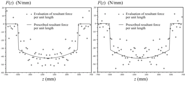
The influence of not modeling the strip is evaluated by considering two diﬀerent contact pressures having the same resultant forces per unit length denoted by Fp(z). It is shown that the method does not depend on the detailed contact repartition but only on the resultant forces per unit length Fp(z). Since the inverse method enables to evaluate the resultant forces per unit length regardless of real local contact repartitions, the residual stress profile in the strip is available with (2) and (3) without modeling the contact and the strip. The relationship between the resultant forces per unit length and the residual stress profile in the strip is obtained by simple string equilibrium of the strip, which holds only if shear stress is negligible in the strip. This latter condition is satisfied because very thin strips are considered.

The two diﬀerent contact pressures having the same resultant forces per unit length are denoted in the follow-ing by "quadratic conditions" and "constant conditions" because the local pressure repartitions are respectively quadratic or constant with respect to the circumferential direction as shown in Figure 8. Very similar results (eval-uation of the resultant forces per unit length profile along the axial direction) are obtained for both conditions. Equations (2) and (3) give a relationship between the resultant forces per unit length and the residual stress profile in the strip. Thus, the prescribed resultant forces per unit length profile Fp_{(z) (shown in Figure 9a) is set so that it}

(15)

0 -0.4 -0.2 0.2 0.4 -0.5 -0.3 -0.1 0.1 0.3 0.5 0 -1 -1.4 -1.2 -0.8 -0.6 -0.4 -0.2 -1.3 -1.1 -0.9 -0.7 -0.5 -0.3 -0.1 φ (rad) s

Contact pressure (MPa)

z=-490 mm z=-455 mm z=-420 mm z=-385 mm

(a) Quadratic conditions

0 -0.4 -0.2 0.2 0.4 -0.5 -0.3 -0.1 0.1 0.3 0.5 0 -0.8 -0.6 -0.4 -0.2 -0.7 -0.5 -0.3 -0.1 φ (rad) s

Contact pressure (MPa)

z=-490 mm z=-455 mm z=-420 mm z=-385 mm

(b) Constant conditions

Figure 8: Prescribed contact pressure

-700 -500 -300 -100 100 300 500 700 0 -40 -20 -30 -10 -45 -35 -25 -15 -5 F (z) (N/mm)p z (mm)

(a) Prescribed resultant forces profile Fp_(z)

0 200 100 20 40 60 80 120 140 160 180 -700 -500 -300 -100 100 300 500 700 σ (z) (MPa)ss z _(mm)

(b) Corresponding long edges defect in the strip

Figure 9: Prescribed long edges defect

From the direct problem, synthetic data um

x and umy are extracted at the hole surface and presented at several

axial positions in Figure 10. In order to be consistent with a possible measurement system only a few points (around 10) are considered for the inputs for the inverse method as show in Figure 11. Then the inverse method presented in this paper is applied at each axial position of the mesh. Since symmetric pressures are applied with respect to the circumferential direction Fy = 0, thus Fxis compared with Fp and the accuracy of the method is

determined by the mean value of relative errors along the axial direction:

Err= 100 v u u t∫L −L[F(z)− Fp(z)] 2_dz ∫L −L [ FP_(z)]2_dz (33)

Measurements are carried out practically with noise. In order to evaluate noise sensitivity, random numbers are added to the inputs. Capacitive probes have a very high resolution and can measure variations of displacements under 1 nm. Thus, three levels of noise are considered, with respective amplitude 0.01µm (which corresponds to 10 times the resolution of capacitive probes), 0.1µm (100 times the resolution) and 0.3 µm (300 times the resolution). Examples of noisy inputs are given in Figure 12. Results without and with noise are presented in Figure 14 and quantified errors are listed in Table 3. Results are satisfying for the two first noise conditions, but the method fails for the third one (amplitude 0.3µm). The measurement system should be designed such as the level of noise does not exceed 0.1µm. The method converges with only 3 terms in the sums as demonstrated in Figure 13. This truncation number is the same for noisy inputs since it corresponds to a strong regularization.

(16)

Model parameters, listed in Table 2, have been chosen in order to be consistent with rolling process dimensions such as strip width, thickness, roll radius and length. The hole dimension has been set so that it seems technically possible to drill the hole under the roll surface. The inversion quality depends on the detecting roll design pa-rameters. A convenient design is presented in this Section. Diﬀerent designs are also studied in Section 5, where parameter b is varying from 148 mm to 138 mm. Sensitivity with respect to geometrical parameters are therefore highlighted. 0 -2 2 -3 -2.5 -1.5 -1 -0.5 0.5 1 1.5 2.5 3 0 -10 -8 -6 -4 -2 -11 -9 -7 -5 -3 -1 φ (rad)_i z=-490 mm z=-455 mm z=-420 mm z=-385 mm u (μm)_xm

(a) Quadratic conditions um x 0 -2 2 -3 -2.5 -1.5 -1 -0.5 0.5 1 1.5 2.5 3 0 -8 -6 -4 -2 -9 -7 -5 -3 -1 φ (rad)_i z=-490 mm z=-455 mm z=-420 mm z=-385 mm u (μm)_xm (b) Constant conditions um x 0 -2 2 -3 -2.5 -1.5 -1 -0.5 0.5 1 1.5 2.5 3 0 1 -0.8 -0.6 -0.4 -0.2 0.2 0.4 0.6 0.8 φ (rad) i z=-455 mm z=-420 mm z=-385 mm z=-490 mm u (μm)_ym (c) Quadratic conditions um y 0 -2 2 -3 -2.5 -1.5 -1 -0.5 0.5 1 1.5 2.5 3 0 -0.6 -0.4 -0.2 0.2 0.4 0.6 0.8 -0.7 -0.5 -0.3 -0.1 0.1 0.3 0.5 0.7 φ (rad) i z=-455 mm z=-420 mm z=-385 mm z=-490 mm u (μm)_ym (d) Constant conditions um y Figure 10: Displacements from FEM extracted at the hole surface for long edges defect

0 -4 -3 -2 -1 1 2 3 4 0 -10 -12 -8 -6 -4 -2 -11 -9 -7 -5 -3 -1 φ (rad) i z=-490 mm u (μm)xm

(a) Quadratic conditions um x 0 -4 -3 -2 -1 1 2 3 4 0 -1 1 -0.8 -0.6 -0.4 -0.2 0.2 0.4 0.6 0.8 φ (rad) i z=-490 mm u (μm)_ym (b) Quadratic conditions um y Figure 11: A few points extracted from displacements for long edges defect

(17)

-7 -6 -5 -4 -3 -2 -1 -0 -4 -3 -2 -1 0 1 2 3 4 φ (rad)_i z=-385 mm u (μm)xm 0.3 μm Noise amplitude 0.1 μm 0.01 μm

(a) Noisy inputs um

x, z= −385 mm -0.8 -0.6 -0.4 -0.2 0.0 0.2 0.4 0.6 -4 -3 -2 -1 0 1 2 3 4 φ (rad) i z=-385 mm u (μm)_ym 0.3 μm Noise amplitude 0.1 μm 0.01 μm (b) Noisy inputs um y, z= −385 mm -2.0 -1.5 -1.0 -0.5 -4 -3 -2 -1 0 1 2 3 4 φ (rad)_i z=-192.5 mm u (μm)xm 0.3 μm Noise amplitude 0.1 μm 0.01 μm (c) Noisy inputs um x, z= −192.5 mm -0.3 -0.2 -0.1 0.0 0.1 0.2 0.3 -4 -3 -2 -1 0 1 2 3 4 φ (rad) i z=-192.5 mm u (μm)_ym 0.3 μm Noise amplitude 0.1 μm 0.01 μm (d) Noisy inputs um y, z= −192.5 mm Figure 12: Noisy inputs (constant condition) for long edges defect

(18)

-700 -500 -300 -100 100 300 500 700 0 -80 -60 -40 -20 -70 -50 -30 -10 10

Number of terms

in the sums

4

3

2

1

F (z) (N/mm)

x

F (z)

p

z (mm)

Figure 13: Convergence of the inverse method for quadratic conditions

Table 3: Error estimate for long edges defect

Noise amplitude Quadratic conditions Constant conditions

Without noise 4.12 % 4.5%

0.01µm 4.3 % 4.6 %

0.1µm 5.7 % 8.35 %

(19)

0 -40 -20 -30 -10 -45 -35 -25 -15 -5 5 -700 -500 -300 -100 100 300 500 700 F(z) (N/mm) z (mm)

Evaluation of resultant force per unit length

Prescribed resultant force per unit length

(a) Quadratic conditions, without noise

0 -40 -20 -30 -10 -45 -35 -25 -15 -5 5 -700 -500 -300 -100 100 300 500 700 F(z) (N/mm) z (mm)

(b) Constant conditions, without noise

-45 -40 -35 -30 -25 -20 -15 -10 -5 0 5F(z) (N/mm) z (mm)

-700 -500 -300 -100 100 300 500 700

(c) Quadratic conditions, noise amplitude 0.01µm

-45 -40 -35 -30 -25 -20 -15 -10 -5 0 5F(z) (N/mm) z (mm)

-700 -500 -300 -100 100 300 500 700

(d) Constant conditions, noise amplitude 0.01µm

-50 -40 -30 -20 -10 0 10 F(z) (N/mm) z (mm)

-700 -500 -300 -100 100 300 500 700

(e) Quadratic conditions, noise amplitude 0.1µm

-45 -40 -35 -30 -25 -20 -15 -10 -5 0 5F(z) (N/mm) z (mm)

-700 -500 -300 -100 100 300 500 700

(20)

-50 -40 -30 -20 -10 0 10 20 F(z) (N/mm) z (mm)

-700 -500 -300 -100 100 300 500 700

(g) Quadratic conditions, noise amplitude 0.3µm

-50 -40 -30 -20 -10 0 10 F(z) (N/mm) z (mm)

-700 -500 -300 -100 100 300 500 700

(h) Constant conditions, noise amplitude 0.3µm

Figure 14: Reconstruction of resultant forces per unit length for long edges defect

4.2. Long center defect

A second numerical example is given where the prescribed resultant forces per unit length Fp_{(z) correspond}

to a long center defect in the strip as presented in Figure 15. As mentioned the relationship between the resultant forces per unit length and the residual stress profile in the strip is given by (2) and (3). Both quadratic and constant local contact pressures are tested. Displacements extracted from the FE simulation at the hole surface are presented at several axial positions in Figure 16. Then, 10 points are taken into account in these displacements as presented in Figure 11. Measurement noise sensitivity is investigated alike in the previous section for long edges defects, thus three level of noise are considered (0.01µm, 0.1 µm and 0.3 µm). Noisy inputs are similar to those presented in Figure 12. Finally, reconstructions of resultant forces per unit length along the axial direction are presented in Figure 17 for both quadratic and constant conditions, without and with noise on the inputs. Error estimates are given in Table 4. Similar results to the long edges defect conditions are obtained. Noise amplitudes under 0.1µm do not compromise the method.

0 -40 -20 -30 -10 -45 -35 -25 -15 -5 -700 -500 -300 -100 100 300 500 700 F (z) (N/mm)p z (mm)

(a) Prescribed resultant forces profile Fp_(z)

0 100 20 40 60 80 120 140 160 180 -700 -500 -300 -100 100 300 500 700 σ (z) (MPa)ss z _(mm)

(b) Corresponding long center defect in the strip

(21)

0 -2 2 -3 -2.5 -1.5 -1 -0.5 0.5 1 1.5 2.5 3 0 -10 -14 -12 -8 -6 -4 -2 -15 -13 -11 -9 -7 -5 -3 -1 φ (rad) i z=-490 mm z=-455 mm z=-420 mm z=-385 mm u (μm)xm

(a) Quadratic conditions um x 0 -2 2 -3 -2.5 -1.5 -1 -0.5 0.5 1 1.5 2.5 3 0 -10 -8 -6 -4 -2 -11 -9 -7 -5 -3 -1 φ (rad) i z=-490 mm z=-455 mm z=-420 mm z=-385 mm u (μm)xm (b) Constant conditions um x 0 -2 2 -3 -2.5 -1.5 -1 -0.5 0.5 1 1.5 2.5 3 0 -1 1 -1.4 -1.2 -0.8 -0.6 -0.4 -0.2 0.2 0.4 0.6 0.8 1.2 1.4 φ (rad) i z=-455 mm z=-420 mm z=-385 mm z=-490 mm u (μm)_ym (c) Quadratic conditions um y 0 -2 2 -3 -2.5 -1.5 -1 -0.5 0.5 1 1.5 2.5 3 0 -0.8 -0.6 -0.4 -0.2 0.2 0.4 0.6 0.8 φ (rad) i z=-455 mm z=-420 mm z=-385 mm z=-490 mm u (μm)_ym (d) Constant conditions um y Figure 16: Displacements from FEM extracted at the hole surface for long center defect

(22)

0 -40 -20 -30 -10 -45 -35 -25 -15 -5 5 -700 -500 -300 -100 100 300 500 700 F(z) (N/mm) z (mm)

(a) Quadratic conditions, without noise

0 -40 -20 -30 -10 -45 -35 -25 -15 -5 5 -700 -500 -300 -100 100 300 500 700 F(z) (N/mm) z (mm)

(b) Constant conditions, without noise

-45 -40 -35 -30 -25 -20 -15 -10 -5 0 5 -700 -500 -300 -100 100 300 500 700 F(z) (N/mm) z (mm)

(c) Quadratic conditions, noise amplitude 0.01µm

-45 -40 -35 -30 -25 -20 -15 -10 -5 0 5 -700 -500 -300 -100 100 300 500 700 F(z) (N/mm) z (mm)

(d) Constant conditions, noise amplitude 0.01µm

-50 -40 -30 -20 -10 0 10 -700 -500 -300 -100 100 300 500 700 F(z) (N/mm) z (mm)

(e) Quadratic conditions, noise amplitude 0.1µm

-50 -40 -30 -20 -10 0 10 -700 -500 -300 -100 100 300 500 700 F(z) (N/mm) z (mm)

(23)

-60 -50 -40 -30 -20 -10 0 10 20 -700 -500 -300 -100 100 300 500 700 F(z) (N/mm) z (mm)

(g) Quadratic conditions, noise amplitude 0.3µm

-60 -50 -40 -30 -20 -10 0 10 20 -700 -500 -300 -100 100 300 500 700 F(z) (N/mm) z (mm)

(h) Constant conditions, noise amplitude 0.3µm

Figure 17: Reconstruction of resultant forces per unit length for long center defect

Table 4: Error estimate for long center defect

Noise amplitude Quadratic conditions Constant conditions

Without noise 0.5 % 0.5%

0.01µm 0.52 % 0.52 %

0.1µm 1.1 % 0.9 %

0.3µm 6.7 % 7.15 %

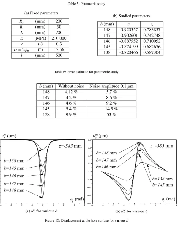
5. Parametric study

In this section a parametric study with respect to the position of the hole center b is presented in order to highlight geometrical constrains. The parameter b is varying from 148 mm (alike in Section 4) to 138 mm. Thus, several FE computations have been performed with geometrical and mechanical parameters listed in Table 5a and five diﬀerent values of b listed in Table 5b. It is clear that the method quality is a compromise between the amplitude of displacements at the hole surface and the parameters ri and a as mentioned at the beginning of

Section 4. When b decreases, riand a also decrease. There is a regularization eﬀect due to the fact that a becomes

more and more diﬀerent from 1, which reduces the instability due to factors 1/(1 − a2). This latter regularization competes with the fact that the amplitude of displacements at the hole surface decreases which tends to degrade the integrals quality of (13) and increase errors amplitudes. Displacements at the hole surface are presented in Figure 18 at the axial position z= −385 mm for the five values of b. In the meanwhile ridecreases, thus errors are

amplified by 1/rk_i which becomes greater and greater when b decreases, however since the sums are truncated at only three terms this latter instability eﬀect is not prevailing. Results for the same long edges defect as presented in Section 4 for quadratic conditions are presented in Figure 19 and errors are listed in Table 6, for both conditions without noise and with perturbed inputs with 0.1µm amplitude. Accuracy decreases and noise sensitivity increases rapidly when b decreases. It is reasonable for this set of design parameters to fix b= 148 mm in order to ensure a good reconstruction quality.

(24)

Table 5: Parametric study

(a) Fixed parameters

Rs (mm) 200 Ri (mm) 50 L (mm) 700 E (MPa) 210 000 ν (-) 0.3 α = 2φ0 (◦) 13.56 l (mm) 500 (b) Studied parameters b (mm) a ri 148 -0.920357 0.783857 147 -0.902601 0.742748 146 -0.887552 0.710052 145 -0.874199 0.682676 138 -0.820466 0.587304

Table 6: Error estimate for parametric study

b (mm) Without noise Noise amplitude 0.1µm

148 4.12 % 5.7 % 147 4.2 % 8.6 % 146 4.6 % 9.2 % 145 5.4 % 14.5 % 138 9.9 % 53 % -9 -8 -7 -6 -5 -4 -3 -2 -1 -0 -4 -3 -2 -1 0 1 2 3 4 φ (rad)_i b=147 mm b=146 mm b=145 mm b=138 mm u (μm)xm b=148 mm

z=-385 mm

(a) um x for various b -0.8 -0.6 -0.4 -0.2 0.0 0.2 0.4 0.6 0.8 -4 -3 -2 -1 0 1 2 3 4 φ (rad) i b=147 mm b=146 mm b=145 mm b=138 mm u (μm)ym b=148 mm

z=-385 mm

(b) um y for various b Figure 18: Displacement at the hole surface for various b

(25)

0 -40 -20 -30 -10 -45 -35 -25 -15 -5 5 -700 -500 -300 -100 100 300 500 700 F(z) (N/mm) z (mm)

(a) b= 148 mm, without noise

-50 -40 -30 -20 -10 0 10 F(z) (N/mm) z (mm)

-700 -500 -300 -100 100 300 500 700 (b) b= 148 mm, noise amplitude 0.1 µm 0 -40 -20 -30 -10 -45 -35 -25 -15 -5 5 -700 -500 -300 -100 100 300 500 700 F(z) (N/mm) z (mm)

(c) b= 147 mm, without noise 0 -40 -20 -50 -30 -10 10 -45 -35 -25 -15 -5 5 F(z) (N/mm) z (mm)

-700 -500 -300 -100 100 300 500 700 (d) b= 147 mm, noise amplitude 0.1 µm 0 -40 -20 -30 -10 -45 -35 -25 -15 -5 5 -700 -500 -300 -100 100 300 500 700 F(z) (N/mm) z (mm)

(e) b= 146 mm, without noise

0 -40 -20 -50 -30 -10 10 -45 -35 -25 -15 -5 5 F(z) (N/mm) z (mm)

-700 -500 -300 -100 100 300 500 700

(26)

0 -40 -20 -50 -30 -10 -45 -35 -25 -15 -5 5 -700 -500 -300 -100 100 300 500 700 F(z) (N/mm) z (mm)

(g) b= 145 mm, without noise 0 -40 -20 20 -50 -30 -10 10 -45 -35 -25 -15 -5 5 15 F(z) (N/mm) z (mm)

-700 -500 -300 -100 100 300 500 700 (h) b= 145 mm, noise amplitude 0.1 µm 0 -40 -20 -30 -10 -35 -25 -15 -5 5 -700 -500 -300 -100 100 300 500 700 F(z) (N/mm) z (mm)

(i) b= 138 mm, without noise

0 -40 -20 20 -30 -10 10 30 -35 -25 -15 -5 5 15 25 F(z) (N/mm) z (mm)

-700 -500 -300 -100 100 300 500 700

(j) b= 138 mm, noise amplitude 0.1 µm

Figure 19: Reconstruction for long edges defect and diﬀerent values of b

6. Conclusion

A semi-analytical inverse method based on complex plane elasticity and conformal mapping techniques has been developed and tested by numerical examples. Application of this inverse method to latent flatness defect detection during rolling process has been considered (long edges and long center defects have been tested). Con-sistent quantity is evaluated (resultant forces per unit length profile along the axial position) in order to infer residual stress profile in steel strips. Good accuracy is observed and the added noise under 0.1µm amplitude (which corresponds to 100 times the resolution of capacitive probes) does not compromise the method. This work encourages further technical developments for a feasible measurement system dedicated to the aimed application. In this paper a Möbius transformation has been used, but more generally the same principles can be used for other geometries and other conformal mappings. The key point is the Riemann mapping theorem that ensures that one can transform any plane geometry simply or doubly-connected into a disk or an annulus respectively. Thus (9) arises for the inverse Cauchy problem where displacements and surface tractions are known on the internal or external surface. Therefore by adding both equations of (9) one holomorphic potential is directly identified, then the other one is obtained. Thus semi-analytical inverse solution can be established, alike the presented developments.

7. Acknowledgement

The author takes the opportunity to acknowledge Alain Ehrlacher (Laboratoire Navier), Nicolas Legrand (ArcelorMittal research and development) and Caio Pereira Santos (Ecole des Ponts ParisTech) for their ideas and fruitful discussions.

(27)

References

Abdelkhalek, S., Montmitonnet, P., Legrand, N., Buessler, P., 2011. Coupled approach for flatness prediction in cold rolling of thin strip. International Journal of Mechanical Sciences 53, 661–675.

Andrieux, S., Baranger, T.N., 2008. An energy error-based method for the resolution of the cauchy problem in 3d linear elasticity. Computer Methods in Applied Mechanics and Engineering 197, 902 – 920.

Bellis, C., Bonnet, M., 2010. A fem-based topological sensitivity approach for fast qualitative identification of buried cavities from elastodynamic overdetermined boundary data. International Journal of Solids and Struc-tures 47, 1221–1242.

Berger, B., Mucke, G., Neuschutz, E., Thies, H., 1991. Deflection measuring roller. US Patent 4,989,457.

Berger, B., Mucke, G., Thies, H., Neuschutz, E., 1983. Apparatus for measuring stress distribution across the width of flexible strip. US Patent 4,366,720.

Bingqiang, Y., Hongmin, L., Lipo, Y., Yan, P., Zhiming, L., 2009. A new type of contact shape meter and its in-dustry application, in: Measuring Technology and Mechatronics Automation, 2009. ICMTMA’09. International Conference on, IEEE. pp. 20–23.

Börchers, J., Gromov, A., 2008. Topometric measurement of the flatness of rolled products - the system topplan. Mettalurgist 52, 247–252.

CEA, 2011. Cast3m. Commissariat A l’Energie Atomique, http://www-cast3m.cea.fr/.

Dahlberg, C., Jonsson, L., 2006. Seamless Stressometer Roll Eliminating the Strip marking and flatness mea-surement dilemma, in: Achieving Profile and flatness in flat products, The Institute of Materials, Minerals and Mining. Achieving Profile and flatness in flat products, Birmingham UK, JAN 24-25, 2006.

Delvare, F., Cimetière, A., Hanus, J.L., Bailly, P., 2010. An iterative method for the cauchy problem in linear elasticity with fading regularization eﬀect. Computer Methods in Applied Mechanics and Engineering 199, 3336 – 3344.

Delvare, F., Cimetière, A., Pons, F., 2002. An iterative boundary element method for cauchy inverse problems. Computational mechanics 28, 291–302.

Faure, J.P., Malard, T., 2004. Method of and a device for flatness detection. US Patent 6,729,757.

Garcia, D., Garcia, M., Obeso, F., Fernandez, V., 2002. Flatness measurement system based on a nonlinear optical triangulation technique. IEEE Transactions on Instrumentation and Measurment 51, 188–195.

Guodong, X.S.Y.B.H., 2004. Shape meter of pressing magnetic type for cold rolling strip to applicating 4-roller reversible rolling mill. Metallurgical Equipment 5, 010.

Hacquin, A., 1996. Modelisation thermo-mecanique tridimensionnelle du laminage: couplage bande-cylindres [3D thermomechanical modelling of rolling processes: coupling strip and rolls]. Ph.D. thesis. Cemef Ecole des Mines de Paris. In French.

Haddar, H., Kress, R., et al., 2013. A conformal mapping method in inverse obstacle scattering. Complex Variables and Elliptic Equations .

Hassen, F.B., Boukari, Y., Haddar, H., et al., 2010. Inverse impedance boundary problem via the conformal mapping method: the case of small impedances. Revue ARIMA 13, 47–62.

Isakov, V., 1998. Inverse problems for partial diﬀerential equations. volume 127 of Applied mathematical sciences. Springer.

Kipping, M., Franz, R., Tuschhoﬀ, M., Sudau, P., 2000. Planarity measuring roller. US Patent 6,070,472. Kress, R., 2012. Inverse problems and conformal mapping. Complex Variables and Elliptic Equations 57, 301–