Direct modeling of material deposit and identification of energy transfer in gas metal arc welding

HAL Id: hal-00923628

https://hal-mines-paristech.archives-ouvertes.fr/hal-00923628

Submitted on 25 Apr 2014

HAL is a multi-disciplinary open access

archive for the deposit and dissemination of sci-entific research documents, whether they are pub-lished or not. The documents may come from teaching and research institutions in France or abroad, or from public or private research centers.

L’archive ouverte pluridisciplinaire HAL, est destinée au dépôt et à la diffusion de documents scientifiques de niveau recherche, publiés ou non, émanant des établissements d’enseignement et de recherche français ou étrangers, des laboratoires publics ou privés.

Direct modeling of material deposit and identification of

energy transfer in gas metal arc welding

Michel Bellet, Makhlouf Hamide

To cite this version:

Michel Bellet, Makhlouf Hamide. Direct modeling of material deposit and identification of energy transfer in gas metal arc welding. International Journal of Numerical Methods for Heat and Fluid Flow, Emerald, 2013, 23 (8), pp.1340-1355. �10.1108/HFF-01-2012-0018�. �hal-00923628�

Direct Modeling of Material Deposit and Identification of

Energy Transfer in Gas Metal Arc Welding

Michel Bellet, Makhlouf Hamide

MINES ParisTech, CEMEF – Centre de Mise en Forme des Matériaux CNRS UMR 7635, Sophia Antipolis, France

michel.bellet@mines-paristech.fr

Abstract

Purpose – The purpose of this paper is to present original methods related to the modeling of material deposit and associated heat sources for finite element simulation of gas metal arc welding (GMAW).

Design/methodology/approach – The filler deposition results from high frequency impingements of melted droplets. The present modeling approach consists of a time-averaged source term in the mass equation for selected finite elements in the fusion zone. The associated expansion of the mesh is controlled by means of adaptive remeshing. The heat input includes a volume source corresponding to the droplets energy, for which a model from the literature is expressed in coherency with mass supply. Finally, an inverse technique has been developed to identify different model parameters. The objective function includes the differences between calculations and experiments in terms of temperature, but also shape of the fusion zone.

Findings – The proposed approach for the modeling of metal deposition results in a direct calculation of the formation of the weld bead, without any a priori definition of its shape. Application is shown on GMAW of steel 316LN, for which parameters of the model have been identified by the inverse method. They are in agreement with literature and simulation results are found quite close to experimental measurements.

Originality/value – The proposed algorithm for material deposit offers an alternative to the element activation techniques that are commonly used to simulate the deposition of filler metal. The proposed inverse method for parameter identification is original in that it encompasses an efficient and convenient technique to take into account the shape of the fusion zone.

Keywords Welding, Fusion zone, Metal deposition, Heat source, Finite element, Inverse method.

Paper type Research paper

Int. J. Num. Meth. Heat Fluid Flow 23, 8 (2013) 1340-1355. DOI 10.1108/HFF-01-2012-0018

Introduction

In the literature, there are two main approaches in numerical modeling of welding. A first class of models focuses on heat and fluid flow: “HFF” models address the physical phenomena occurring in the fusion zone: buoyancy, capillary and electromagnetic effects (Kim et al., 2003; Cao et al., 2004; Hu et al., 2008). A second class of models - named “TMM” for Thermo-Mechanics and Metallurgy - aims at calculating stresses, strains and microstructural evolutions in assembled parts. They address the coupled heat transfer, metallurgical transformations and mechanical phenomena occurring in the neighborhood of the weld pool, but also at larger scales in welded parts. In such models, the actual physics taking place in the fusion zone is replaced by simplified models. The melted material is considered as a viscoplastic or Newtonian fluid of arbitrary high viscosity, thus ignoring complex fluid flow. In addition, in order to mimic the convective heat transfer occurring in the fusion zone, different methods are used: augmented or anisotropic heat conductivity, additional volume heat source (Goldak, 1986). TMM approaches are widely used - see the three-part review of Lindgren (2001) and (Lindgren, 2006) - but they suffer from a specific limitation regarding the modeling of weld bead formation in the context of gas metal arc welding (GMAW). During GMAW, material deposit results from droplets of melted filler material, falling into the weld pool and forming the joint after solidification. In TMM models, this metal supply is generally modeled by progressive activation of the finite elements that constitute the weld bead, according to the electrode displacement (Lindgren et al., 1999). This approach has three major limitations:

• The geometry of the weld bead is defined a priori;

• The construction of the mesh is painful and time consuming;

• This generally impedes dynamic remeshing.

In the present TMM approach, metal deposition and joint formation are modeled in a more physical way with fewer constraints. The basic idea consists in implementing a source term in the mass equation for some selected elements of the fusion zone. Consistently, a corresponding source term is considered in the energy equation. The paper is organized as follows. Section 1 presents the main features of the TMM method. Section 2 addresses the modeling of material deposit and associated energy transfer. In Section 3, an application is given, including parameter identification by an original inverse finite element method.

1 Thermomechanical Modeling of Arc Welding Processes

The authors have developed a TMM three-dimensional finite element model for arc welding, named TRANSWELD (Pequet et al., 2006; Hamide and Bellet, 2007; Hamide, 2008; Hamide et

al., 2008). It is based on coupled solutions of heat transfer, metallurgical kinetics and mechanics.

Because the present paper focuses on material and energy deposit, the presentation is limited here to the main features of the thermomechanical resolution, which is based upon the approach proposed by Bellet and Fachinotti (2004) and Bellet et al. (2005). See details in references.

• Energy conservation is solved using an enthalpy-based formulation. Each element (tetrahedron) is considered either solid-like or fluid-like, depending on temperature: over the solidus temperature TS, the element is considered liquid-like, below it is solid-like.

• A thermo-viscoplastic (TVP) model is used in liquid-like elements (mushy or liquid state) The model is of power-law type and encompasses the Newtonian behavior in liquid state. A thermo-elastic-viscoplastic (TEVP) model is used in solid-like elements.

• Momentum and mass conservation equations are solved concurrently in a mixed velocity-pressure formulation. The solution provides the material velocity in solid and melted regions, together with stress and strains in solid regions.

• The incremental updating of nodal positions is performed through an arbitrary Lagrangian-Eulerian technique (ALE). Solid nodes are updated using the calculated material velocity. Other nodes are updated by a barycentering method in order to preserve a good element aspect ratio.

• The mesh boundary represents the material surface. An anisotropic remeshing procedure is used from time to time, based upon an error estimator (Hamide et al., 2008).

• At each time increment, the resolution is divided in 4 modules. Step 1: thermal resolution, providing temperature and liquid metal fraction. Step 2: mechanical resolution, providing velocity and pressure fields, and the stress tensor in solid-like elements. Step 3: mesh updating using ALE scheme. Step 4: possible adaptive remeshing.

2 Modeling of Material Deposit

During GMAW, the material deposit results from droplets of melted filler material, arising from the fusion of the consumable electrode. These droplets fall down into the weld pool after they have been accelerated during their flight through the electric arc plasma. The progressive and continuous solidification of the weld pool gives birth to the weld joint. In the next paragraphs, we will give the expressions of the mass input and associated energy input to the fusion zone, corresponding to the impingement of droplets. We will then deduce the appropriate source terms to be considered in the mass and energy equations.

2.1 Modeling of Mass Transfer

2.1.1 Mass flow rate and droplets impingement zone

In GMAW context, the mass flow rate is simply mw w Rw vw

2

π ρ =

& , where R and w v are w

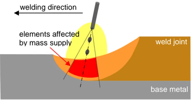
respectively the radius and velocity of the filler wire, ρ_w its density at initial temperature T_0,w. Assuming there is no material loss through the arc plasma, m&_w represents the time-averaged mass flow rate associated with the high-frequency impingement of metal droplets in the fusion zone. Thus, locally in the fusion zone, this time-averaged material supply can be modeled by a source term in the mass conservation equation. A first task consists in selecting elements of the fusion zone that would be affected by such a source term. For this purpose, a virtual cone may be attached to the electrode tip (Figure 1). Selected elements are those in the liquid state and located inside the cone: elements colored in red. However, accelerated melted metal droplets penetrate deeply into the bath. This phenomenon is responsible, together with Marangoni effect, for the characteristic finger-type shape of the weld pool (see Figure 4 in Section 3 for instance). Therefore, rather than a cone, we consider the model suggested by Kumar and Badhuri (1994), after Lancaster (1986). These authors suppose that each droplet impingement generates a cylindrical cavity. Its radius, Rfill, is supposed twice as big as the droplet radius, while its height,

Hfill, can be determined by an energy balance commented hereafter. Rfill is obtained from wire

radius and velocity, and the detachment frequency of the droplets, fd, using mass conservation:

3 1 2 _ _ ) ( 4 3 2 2 _       = = w w f drops w w d f drops fill R v T f R R ρ ρ (1)

fd depends on the shielding gas and welding intensity. Rhee and Kannatey-Asibu (1992) have

shown that the transition from globular to spray-type transfer occurs around 300 A. Their results have been exploited by Kim et al. (2003) who proposed the following sigmoid function:

2 0025 . 0 874 . 0 506 . 323 06437 . 6 086 . 291 exp 1 44 . 243 I I I fd + − +       ₋ + − = (2)

Hence Rfill can be fully determined knowing I, Rw, vw, ρw. Regarding now Hfill, it is determined by

the model of Kumar and Badhuri (1994) which consists in assuming that the energy needed to form such a cavity, that is the work of hydrostatic pressure and liquid surface tension along the cavity wall, is provided by the droplet kinetic energy:

g v R g R g R H drops f drops f f drops f drops fill 3 2 _ _ 2 _ _ +         + − = ρ γ ρ γ ₍₃₎

where g denotes gravity, ρ the density, γ the surface tension, and vdrops_f the impinging velocity.

vdrops_f can in turn be expressed as a function of material and welding parameters. Assuming a

constant acceleration, we get:

arc drops d drops f drops v a L v _ = _ 2 +2 (4)

where vdrops_d is the initial detachment velocity, Larc the arc length and adrops the acceleration,

which can be estimated from the second law of Newton. However, as noted by Jones et al. (1998), it seems preferable to deduce adrops or vdrops_f directly from experiments.

2.1.2 Source term in mass equation

In selected elements, a mass source term is considered. Assuming a uniform distribution of the mass supply, we get:

∑

where v denotes the velocity field, ρ the density and V the volume of each selected element K. K

In a non steady-state simulation, the volume integration of these expansion terms θ&_drops induces an evolution of the surface of the weld pool, which gives birth after solidification to the joint shape. In the ALE context, this directly affects the surface of the mesh. This is controlled by dynamic remeshing to preserve acceptable geometrical properties for the mesh.

2.2 Modeling of Energy Transfer

2.2.1 Global balance

The total welding power is the voltage-intensity product UI. It is supposed that a fraction η is effectively used for the process. This effective power can be separated in two parts. A first part,

wfus

W& , is used to melt the consumable electrode. A second part, W&surf , corresponds to the thermal

power transferred by the arc plasma to the surface of the welded material. This decomposition is characterized by the parameter ηwfus:

η η η η η UI UI W W UI wfus wfus surf wfus ) 1 ( − + = + = & & (6)

The filler is heated from its initial temperature T0,w to the temperature of the droplets when they

detach: Tdrops_d. Assuming a constant specific heat cp,w, we have:

(

)

w

wfus m c T T L

W& = & , ( _ − 0, )+ (7) where L is the latent heat of the wire material. Note that the combination of equations (6) and _w

(7) provides a direct relation between the value of ηwfus and Tdrops_d.

2.2.2 Source term in energy equation

The time-averaged input power to the fusion zone corresponding to impinging droplets has now to be expressed. Let us start from the equation for energy conservation:

0 ) ( ) ( ) ( _{+∇⋅ −∇⋅ ∇ =} ∂ ∂ T k h t h v ρ ρ (8)

where h is the specific enthalpy and k the thermal conductivity. Here, source terms associated with plastic deformation and Joule effect are ignored. In the selected elements K, this equation must be modified.

• First the volumetric expansion due to droplets impingement must be taken into account through equation (5).

• Second, we must consider an energy source term expressing the energy input. The specific enthalpy of droplets when entering the pool being h_drops=c_p,wT_{drops_f} +L_w, and assuming a uniform input in selected elements, the heat source term is:

) ( ) ( _ , _ , w f drops w p drops K K w f drops w p w drops c T L V L T c m w = + = +

∑

Finally, equation (8) becomes:

drops drops h w T k h t h _{ρ θ} ρ _{−∇⋅ ∇ = & −} &      ⋅ ∇ + ∂ ∂ ) ( v (10)

Hence, it should be noticed that the effective energy source term does not derive directly from the distribution of the energy transported by the impinging droplets. It also includes a corrective term arising from the presence of the mass source term in the mass equation: the effective power source takes into account the volumetric expansion.

3 Application and Validation 3.1 GMAW instrumented experiment

The objective of this section is to show that the models described above for material and energy transfer can be validated by comparison with experimental measurements. The case studied here

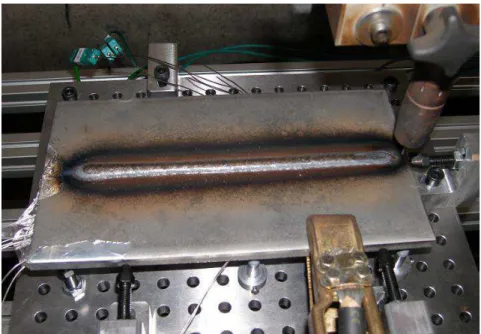
is a "bead-on-plate" test, consisting of a linear single-pass deposit on a plate using a GMA welding process. The base material is the austenitic stainless steel ANSI 316LN. Figure 2 shows an instrumented plate after welding. Figure 3 provides a sketch of the instrumentation. The experiment has been extensively described in the Ph.D. manuscript of Hamide (2008) and in (Aarbogh et al., 2010). The test has been originally designed for validation of thermomechanical simulations of welding and was chosen large enough to obtain a thermal quasi-stationary situation. Here, we focus on material deposit during welding. Mechanical aspects are ignored: the displacement of the plate during and after welding, the formation of strains and stresses are fully presented and discussed in the references just mentioned. The main characteristics of this experiment are the followings:

• Thick plate, 10.5 mm thick, 136 mm wide and 250 mm long (in the welding direction).

• A single pass metal deposit, by GMA welding technique. The electrode is maintained in a vertical position (perpendicular to the upper wide face of the plate). Its total displacement is 230 mm, beginning and finishing at 10 mm from the plate border.

• The arc length Larc (distance between electrode and plate) is maintained constant during

welding: L_arc =10 mm.

• The filler wire material is a 316LSI steel of radius Rw=0.6 mm, feed speed vw =0.2 m/s. • The initial temperature of the plate and of the filler wire is approximately 20°C.

• The process parameters are: welding voltage U =29 V, average welding intensity (controlled automatically) U =360 A, welding speed v_weld =10 mm/s. This yields a nominal welding energy of 1.044 kJ/mm, a welding duration of 23 s.

• The shield gas is M12 (or Arcal 12) argon (Ar) with 1 to 5% CO2.

• The plate is equipped with twelve K-type thermocouples (chromel-alumel, MgO insulated with steel cap) of diameter 1 mm, forced in pre-drilled holes, at locations indicated in Figure 3.

3.2 Experimental Results

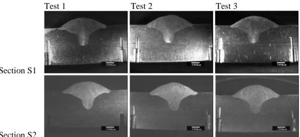
Macrographies of the fusion zone are shown in Figure 4. Issued from three tests performed in the same conditions, and from two transverse sections in the plate, they show a stable and reproducible weld pool shape. The shape is characteristic of steel GMAW with a marked finger-type central penetration. The average experimental values for the width, height and depth of the fusion zone can be found in Table 2.

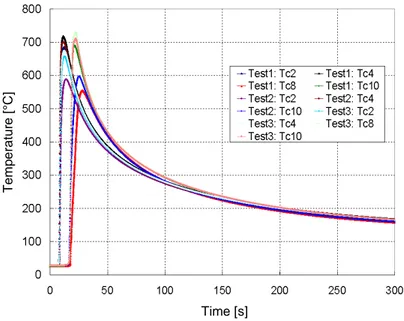
Some temperature measurements by thermocouples (TCs) are reported in Figure 5, see full results in (Aarbogh et al., 2010). These results prove the stationarity of the welding, but also show a certain dispersion, with temperature differences as high as 120°C for TCs at the same nominal distance from the welding line. This can be explained by the effective position of TCs, which can be measured a posteriori. Indeed, significant positioning errors have been recorded, up to 1.5 mm for TC2 in test 2. It can be thought that different contact conditions in drilled holes may also contribute to the observed scattering.

3.3 Modeling Hypotheses and Parameters

The parameters of the different models used in the direct simulation and in the identification procedure for parameter identification are as follows.

• Convection with air and gray-body radiation are assumed on all faces of the plate, with following parameters: heat transfer coefficient h_conv =5 W m-2 K-1, thermal emissivity

25 . 0

= rad

ε , air temperature Tair =20°C.

• The temperature of droplets is supposed to be unchanged during their flight:

d drops f

drops T

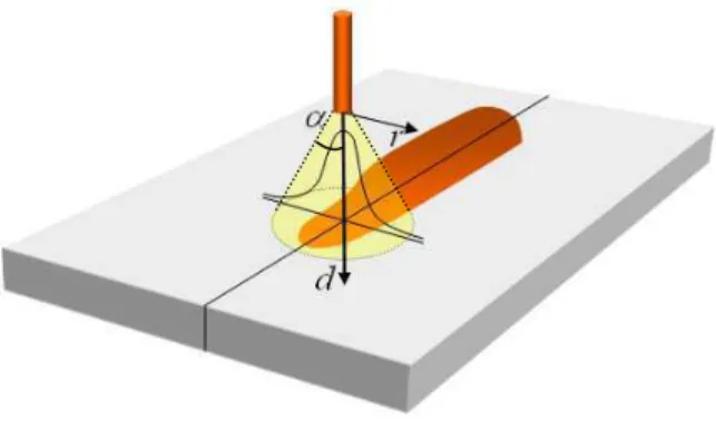
• The arc heating power W&surf transferred to the surface of the plate is modeled by a

Gaussian surface heat source inside a cone of characteristic angle 2α, as illustrated in Figure 6. The corresponding surface heat flux is defined by

      − = 2 2 2 ) tan ( 3 exp ) tan ( 3 ) , ( α α π φ d r d W r d &surf (11)

In this expression, r stands for the radial distance of the studied point at the surface of the metal to the axis of the electrode and d stands for the distance to the electrode along its axial direction (d is then quite close to the arc length Larc).

• The droplet impingement zone is cylindrical, as described in Section 2.1.1. Its dimensions are fixed to Rfill =1.0 mm and Hfill =2.0 mm, according to the following analysis.

o The radius Rfill is determined by equation (1), using an estimation of the droplets

detachment frequency provided by equation (2). The density of the wire metal is taken constant: ρw=7400 kg m

-3

. Using the experimental data of Section 3.1, the following values are obtained: f_d =333 Hz, Rdrops_f =0.55 mm, Rfill =1.09 mm. o The height Hfill is determined by equation (3), using the following parameters. The

surface tension is taken as γ =1 N m-1. The impingement velocity of droplets is estimated by equation (4) in which the detachment velocity is extrapolated from the experimental results obtained by Jones et al. (1998): vdrops_d =1.2 m s

-1

, and the acceleration is assumed constant during transfer and taken from the work of Kim et al. (2003) as: adrops=200 m s

-2

. This yields an estimation of the impingement velocity: v_{drops_f} =2.3 m s-1. Applying equation (3), we obtain

9 . 1 = vhs H mm.

• An arbitrarily increased heat conductivity is used, defined by keff = fkk, where k is the

nominal conductivity of the material and f a multiplicative parameter to be identified. _k

• The simulation is run on a computational domain covering one half of the specimen, respecting the symmetry with respect to the welding line.

• Mesh size parameters are hmin =0.8 mm and hmax =7 mm.

• The full set of material parameters of steel 316LN used for the calculations can be found in (Aarbogh et al., 2010).

3.4 Identification of Parameters and Comparison

Four parameters should be identified: the overall welding heat efficiency η (fraction of power effectively transferred to the plate), the magnification factor for heat conductivity fk, the

semi-angle of the Gaussian heat source α, the fraction of heat power used for the fusion of the filler wire ηwfus. They form the four components of vector q.

An inverse analysis technique is used to identify q. The basic principle of the method is to adjust the values of the parameters in order to minimize the difference between numerical calculations and measurements. This difference is expressed in terms of temperatures but also of the shape of the fusion zone, as explained below. Denoting exp

T the measured temperatures and cal T the calculated ones, a sampling procedure has to be defined in order that they could be compared. The calculated values cal

T of course depend on the set of parameters q and on time t. The

distance with respect to exp

∑∑

where S denotes the number of sensors, k the sensor index, I the number of sampling instants, and i the index for sampling instants.

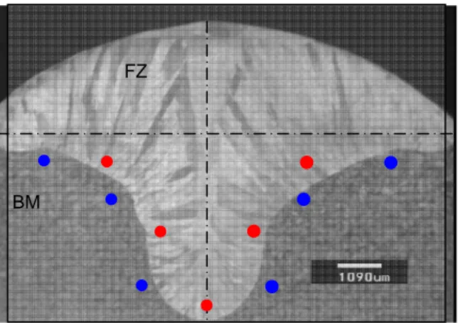
When modeling a welding process, the correct representation of the shape of the weld pool is discriminant in that it reveals the accuracy of the solution provided by the numerical model. With this in view, the function Ψ is complemented with additional terms expressing that at locations where the metal is found melted in the experiment (red dots in Figure 7), the maximum of the calculated temperature should not be found below the liquidus temperature TL. Conversely, at

locations where the metal is found not melted in the experiment (blue dots in Figure 7), the maximum of the calculated temperature should not be found over the solidus temperature TS.

Two additional penalty terms ΨFZ and ΨBM are then expressed as follows:

∑

∑

In these expressions, SFZ denotes the number of selected locations in the fusion zone (red dots),

and SBM the number of selected locations in the non-melted base metal (blue dots). The

expressions between brackets reduce to zero when negative: x =(x+ x)/2. Finally, the modified objective function considered in the present study has the following expression,

      − + − − + × = Ψ

∑

∑

∑∑

The weighting factor β balances temperature and pool shape contributions and is taken as 0.5 in the present work. From the three similar experimental tests presented above, test 3 is chosen as the reference for the identification. The selection of red and blue dots in the fusion zone and in the base metal, respectively, is carried out as follows. The macrographies of the two selected transverse sections of test 3 – shown in Figure 4 – can be analyzed in order to determine the profile of the fusion zone. The right and left profiles of each of the two sections (that is four profiles) are plotted in Figure 8. This allows the determination of several points in the fusion zone and in the base metal, in order to constraint the identification procedure, according to equation (14). In the present case, four points are selected in the fusion zone as well as in the base metal (SFZ =SBM =4). The location of these points is determined arbitrarily, but it can be seen

that they can be selected in order to induce an effective constraint on the solution.

The inverse problem consists then in determining q such that the following function Ψ~(q) be minimized. The minimization problem was solved using the commercial IOSO software (Egorov

et al., 2005), which has been interfaced with the TRANSWELD software in charge of performing

the direct simulations and of calculating the objective function. The optimization took 40 iterations (global CPU time 96 h on Pentium4 @ 2.8 GHz and 1 Gb RAM), yielding the parameter values indicated in Table 1. These parameters are in agreement with values found in the literature (Kumar and DebRoy, 2004), except to a certain extent for the magnification

parameter for the heat conductivity, fk, which is found higher than standard values, typically

found in the range 5 to 15.

η ηwfus tanα fk

0.85 0.35 0.82 19.2

Table 1: Values of parameters issued from automatic identification.

Using equations (6) and (7), an estimation of the droplets temperature can be done. Taking a fixed value c_p,w =700 J kg-1 K-1, ρ_w =7400 kg m-3 and L_w=201897 J kg-1, we get:

2382

_d = drops

T °C, which is in very good agreement with the average droplet temperature of 2400°C determined for mild steel by Jelmorini et al. (1977). This expresses the consistency of the

identified solution.

Figure 9 shows the comparison between calculated and measured temperatures at the three characteristic thermocouple positions of the test: TC3 below the weld bead, TC2 and TC1 respectively 5 and 10 mm aside from the welding line. It can be seen that there is a good global agreement. However, significant differences can be observed during the rapid transient undergone when the electrode passes by the thermocouples. Calculated peak values are systematically higher than measured ones, and the difference increases with temperature. For instance, a rather good agreement is found for the peak temperature at TC1: the measured peak value is 425°C whereas the calculated peak value is 460°C. But the difference is higher at TC3: measured 680°C, calculated 795°C; and even higher at TC2: measured 660°C, calculated 945°C. From these results, two alternative and opposite statements may be expressed:

• A first statement would be that the global model is not capable – even after parameter optimization – of a good global representation of the different phenomena involved: heat and material supply, fusion and solidification, heat transfer. Several causes could be the source of this weakness: erroneous thermophysical properties, too simple Gaussian model for the surface heat source, wrong hypotheses governing the volume heat source, implementation and discretization errors…

• A second statement would be that the direct model fails only for peak values at TCs locations and that this would be due to erroneous recorded temperatures during such rapid transients. The reasons for that can be the size of thermocouples inducing offset times during measurements, the nature of the thermocouples itself creating heat contact resistances between welded wires and magnesia inside sensors, or a too loose contact between thermocouples and the base metal inducing heat contact resistances deep in the drilled holes.

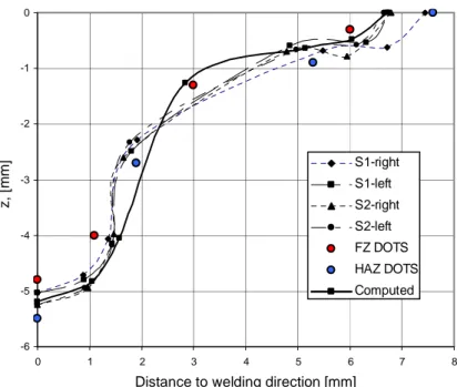
What can help in deciding between those two statements is the quality of the prediction of the fusion zone, as this is part of the global objective function Ψ~. Figure 8 and Figure 10 show the difference between the observed and calculated transverse shape of the fusion zone. It can be seen that the characteristic shape is rather well represented. In particular the width, depth and volume of the fusion zone are in good agreement with the experiment. The shape of the finger part, especially its width variation vs depth shows some difference. This probably results from the fact that it has been chosen here not to optimize the volumetric source, but to determine it on the basis of literature results. It is likely that adding in the identification procedure one or two parameters describing this volumetric source, such as its radius, would lead to a better agreement. However, globally, the predicted characteristic dimensions of the weldment (width, depth, bead height) are quite close to those measured in the two transverse sections, as indicated in Table 2.

[mm] width height depth Exp. Section S1 14.2 2.8 5.0 Exp. Section S2 13.5 2.9 5.2 Calc. 13.4 2.7 5.2

Table 2: Experimental average values of the characteristic dimensions of the fusion zone and predicted values after heat source parameters identification.

This expresses that the combination of the two heat sources, the Gaussian surface source and the cylindrical volume source, is probably a good representation of reality. In view of those results and considering that TCs positions are close enough to the fusion zone and that the thermophysical properties of 316LN are rather well known, our opinion is that between the two opposite statements expressed above, the second one can be validated: the disagreement for peak temperature values is the signature of wrong measurements for very high and fast transient temperatures. Hence the parameters of Table 1 can be validated and accepted as representative parameters for the studied GMA welding process when performed under such conditions. Finally, and as a last result, Figure 11 presents a view of the weld bead formation, as simulated by the present approach.

Conclusion

In this paper, original methods related to the modeling of material deposit and associated heat sources have been proposed for finite element simulation of GMAW in non-steady state conditions. The basic idea consists in implementing a source term in the mass conservation equation for some selected finite elements of the fusion zone. This approach permits the direct modeling of the formation of the weld bead, and thus offers an alternative to the element birth or element activation techniques that are commonly used to simulate the deposition of filler metal. By comparison with such usual methods, the new technique offers a significant advantage: the geometry of the joint does not need to be defined - and consequently meshed - prior to simulation. To be consistent with the above modeling of filler supply, the heat input is split in two contributions. A first contribution is a volume heat source corresponding to the energy transferred through the droplets of filler metal, for which a model taken from the literature is used. It should be noted that a specific expression of the corresponding source term in the energy equation is proposed here in coherency with the expression of mass supply. A second heat input contribution is a surface Gaussian heat source. Because several parameters of the global model have to be identified, an automatic parameter identification technique has been developed. It relies upon an inverse finite element method. The objective function to be minimized includes the differences between calculated and measured temperatures at different locations near the weld, but also penalty terms permitting a convenient and efficient comparison between the calculated and observed shapes of the fusion zone in the transverse section. Application has been shown on GMAW of steel 316LN, for which the optimized set of parameters leads to a good agreement for temperatures and weld pool shape.

Acknowledgement

References

Aarbogh, H.M., Hamide, M., Fjaer, H.G., Mo, A. and Bellet, M. (2010), "Experimental validation of finite element codes for welding deformations", J. Mat. Proc. Tech., Vol. 210, pp. 1681-1689.

Bellet, M. and Fachinotti, V.D. (2004), "ALE method for solidification modelling", Comput. Meth. Appl. Mech. Eng., Vol. 193, pp. 4355-4381.

Bellet, M., Jaouen, O. and Poitrault, I. (2005), "An ALE-FEM approach to the thermomechanics of solidification processes with application to the prediction of pipe shrinkage", Int. J. Num. Methods Heat Fluid Flow, Vol. 15, pp. 120-142.

Cao, Z., Yang, Z. and Chen, X.L. (2004), "Three-dimensional simulation of transient GMA weld pool with free surface", Welding J., June (supplement), pp. 169S-176S.

Egorov, I.N., Kretinin, G.V., Leshchenko, I.A. and Kuptzov, S.V. (2005), "Optimization of complex technical systems", Proc. 9th Int. Conf. on 'Computer Aided Optimum Design in Engineering', Skiathos, Greece, May 2005, Wessex Institute of Technology, pp. 335-340.

Goldak, J. (1986), "Computer modelling of heat flow in welds", Metall. Trans. B, Vol. 17, pp. 587-600.

Hamide, M. and Bellet, M. (2007), "Adaptive mesh technique for coupled problems. Application to welding simulation", Proc. 9th Int. Conf. on Numerical Methods in Industrial Forming Processes, Porto, Portugal, American Institute of Physics, pp. 1561-1566.

Hamide, M., Massoni, E. and Bellet, M. (2008), "Adaptive mesh technique for thermal-metallurgical numerical simulation of arc welding processes", Int. J. Num. Meth. Engng., Vol. 73, pp. 624-641.

Hamide, M. (2008), "Modélisation numérique du soudage à l'arc des aciers", PhD thesis, MINES ParisTech, France. Hu, J., Guo, H. and Tsai, H.L. (2008), "Weld pool dynamics and the formation of ripples in 3D gas metal arc welding", Int. J. Heat Mass Transfer, Vol. 51, pp. 2537-2552.

Jelmorini, G., Tichelaar, G.W. and van den Heuvel, G.J.P.M. (1977), "Droplet temperature measurements in arc welding", Report 212-411-77, Int. Institute of Welding (IIW), 22 pages.

Jones, L.A., Eagar, T.W. and Lang, J.H. (1998), "A dynamic model of drops detaching from a gas metal arc welding electrode", J. Phys. D: Appl. Phys., Vol. 31, pp. 107-123.

Kim, C.H., Zhang, W. and DebRoy, T. (2003), "Modeling of temperature field and solidified surface profile during gas-metal arc fillet welding", J. Appl. Phys., Vol. 94, pp. 2667-2679.

Kumar, S. and Bhaduri, S.C. (1994), "Three-dimensional finite element modeling of gas metal arc welding", Metall. Mater. Trans B, Vol. 25, pp. 435-441.

Kumar, A. and DebRoy, T. (2004), "Guaranteed fillet weld geometry from heat transfer model and multivariable optimization", Int. J. Heat Mass Transfer, Vol. 47, pp. 5793-5806.

Lancaster, J.F. (1986), The Physics of Welding, Pergamon Press, New York.

Lindgren, L.E., Runnemalm, H. and Näsström, M. (1999), "Simulation of multipass welding of a thick plate", Int. J. Num. Methods Eng., Vol. 44, pp. 1301-1316.

Lindgren, L.E. (2001), "Finite element modelling and simulation of welding. Part 1: Increased complexity; Part 2: Improved material modelling; Part 3: Efficiency and integration", J. Thermal Stresses, Vol. 24, pp. 141-192; 195-231; 305-334.

Pequet, C., Lasne, P., Hamide, M., Massoni, E. and Bellet, M. (2006), "A coupled approach for the modelling of arc welding processes", Proc. 11th Int. Conf. on Modeling of Casting, Welding and Advanced Solidification Processes, Opio, Gandin, Ch.-A. and Bellet, M. (eds.), The Minerals, Metals & Materials Society, pp. 855-862.

Rhee, S. and Kannatey-Asibu Jr., E. (1992), "Observation of metal transfer during gas metal arc welding", Weld. J., Vol. 71, pp. 381S-386S.

Figure 1: Schematic representation for the modeling of material deposit in GMA welding. base metal weld joint elements affected by mass supply welding direction

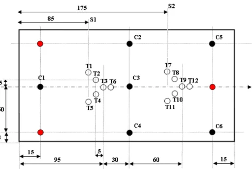
Figure 3: Instrumentation of the plate. White dots labelled "Tx" indicate the location of 12 thermocouples. Thermocouples below the weldment (3, 6, 9, 12) are located at 5.5 mm below the upper surface; others are located 3.5 mm below. Red dots not labelled indicate 3 supporting pins. Black dots labelled "Cx" indicate 6 LVDT sensors following the vertical displacement of the lower face of the plate (not used in this study).All dimensions in mm.

Test 1 Test 2 Test 3

Section S1

Section S2

Figure 4: Macrographies showing the shape of fusion zones from three tests, along transverse sections S1 (top line) and S2 (bottom line) as indicated in Figure 3. Pre-drilled holes for the placement of thermocouples are visible.

Figure 5: Temperature measurements at thermocouples 2, 4, 8 and 10 for three different tests. TCs 2 and 4 form a first peak at 9 s, followed by a second peak for TCs 8 and 10 at 18 s.

Time [s] T e m p e ra tu re [ °C ]

Figure 6: Schematic representation of the Gaussian distribution of the heat surface flux corresponding to the heat transfer from the arc to the plate.

Figure 7: Principle of selection of locations in the fusion zone (FZ, marked by red dots) and in the base metal (BM, blue dots) in view of inverse analysis for heat source identification.

BM

-6 -5 -4 -3 -2 -1 0 0 1 2 3 4 5 6 7 8

Distance to welding direction [mm]

z

[

m

m

]

Figure 8: Profiles of the fusion zone, computed and as deduced from macrographies of test 3 shown in Figure 4. Right and left profiles of sections S1 and S2 are plotted. The horizontal coordinate represents the distance to the welding symmetry plane, as deduced from the macrographies. The vertical coordinate is the distance to the upper surface of the plate. The figure shows the location of red and blue dots in the fusion zone and the base metal, respectively. S1-right S1-left S2-right S2-left FZ DOTS HAZ DOTS Computed

Distance to welding direction [mm]

z

,

[m

m

0

100

200

300

400

500

600

700

800

900

1000

0

50

_{Temps (s)}

100

150

200

Tc1: Numérique

Tc2: Numérique

Tc3: Numérique

Tc1 : Exp

Tc2 : Exp

Tc3 : Exp

Figure 9: Experimental and numerical temperature evolution at different selected locations.

calculated

calculated

calculated

100

Time [s]

T

e

m

p

e

ra

tu

re

[

°C

]

Section S1 Section S2

Figure 10: Calculated (on the left) and observed shapes of the fusion zone (on the right, transverse sections S1 and S2 of test 3). Red color indicates temperatures greater than the solidus temperature (1420°C).

Figure 11: Temperature distribution and adapted finite element mesh.

1397 1550