HAL Id: hal-01142106
https://hal.sorbonne-universite.fr/hal-01142106
Submitted on 14 Apr 2015
HAL is a multi-disciplinary open access archive for the deposit and dissemination of sci-entific research documents, whether they are pub-lished or not. The documents may come from teaching and research institutions in France or abroad, or from public or private research centers.
L’archive ouverte pluridisciplinaire HAL, est destinée au dépôt et à la diffusion de documents scientifiques de niveau recherche, publiés ou non, émanant des établissements d’enseignement et de recherche français ou étrangers, des laboratoires publics ou privés.
Using airborne thermal inertia mapping to analyze the
soil spatial variability at regional scale
I. Cousin, C. Pasquier, M. Séger, A. Tabbagh
To cite this version:
I. Cousin, C. Pasquier, M. Séger, A. Tabbagh. Using airborne thermal inertia mapping to analyze the soil spatial variability at regional scale. Globalsoilmap : basis of the gloabl spatial soil information system : Proceedings of the 1rst Global soilmap conference, Oct 2013, Orléans, France. pp.441-446. �hal-01142106�
1 INTRODUCTION
To describe soil physical characteristics on surface areas, a wide panel of remote sensing and ground based methods has been developed: remote sensing, in the visible and radar domains enable the estima-tion of soil parameters over large areas but they are often limited to the estimation of parameters of the soil surface or the soil surface horizon. On the con-trary, ground based methods, like electrical resistivi-ty or EMI methods, enable to derive soil parameters for the whole soil thickness, i.e. down to about 2 m. Nevertheless, they can hardly be run over large areas of several square kilometers if we intend of keeping a correct resolution of information over the 1 to 2 meters soil depth. The present study focuses on the thermal airborne remote sensing method. It is sup-posed to investigate over the whole soil thickness, and can cover large areas of several square kilome-ters. To evaluate the depth of investigation of the method, this concept being understood as the thick-ness of the soil layers taken into account in a meas-urement-, the measurements of the surface tempera-ture variations will be compared with electrical resistivity measurements recorded for three increas-ing depths of investigation. To determine the pedo-logical parameters that influence the thermal air-borne remote sensing method data, the latter will be compared to local measurements of some pedologi-cal characteristics.
2 THE SOIL SURFACE TEMPERATURE EVOLUTION
The absolute value of the surface temperature of a bare soil depends on several parameters that deter-mine the heat balance at ground surface. They cannot be controlled but lateral changes in the ground ther-mal properties may generate variations in surface temperature that can be measured. The latter are re-lated to the ability of the heat to be moved down-ward or updown-ward by the subsoil. For a homogeneous solid and unsteady heat inputs, the temperature changes are inversely proportional to the thermal in-ertia, and it is thus usual to discuss the results of a thermal prospection in terms of variations in appar-ent thermal inertia (Price, 1977) of the soil. It is of great importance to evaluate the conditions under which the depth of investigation of the method will overpass the first layer (Scollar et al., 1990). This depth does not depend on the choice of a frequency or of other instrument parameters but on the history of the heat exchange at the soil surface before the measurement time: if the duration of a transient in-put of heat (respectively outin-put) lasts one or two days, the depth of investigation would be limited to about 25 cm; it would reach about 1 m if the transi-ent input lasts one week or more. The soil tempera-ture has then to be monitored for several days to
de-Using airborne thermal inertia mapping to analyze the soil spatial
variability at regional scale
I. Cousin, C. Pasquier & M. Séger
INRA, UR0272 SOLS, Orléans, France
A. Tabbagh
UMR 7619 Sisyphe, Paris, France
ABSTRACT: This study aims at demonstrating the ability of thermal airborne remote sensing to help in delin-eating soil types over large areas. Measurements of the surface temperature variations were compared with electrical resistivity measurements recorded for three depths of investigation. The study area was located in the Beauce region with Calcisols and Cambisols, 0.3 to 1.2 m thick. Airborne thermal measurements were recorded by the ARIES radiometer in the 10.5-12.5 µm thermal infra-red channel, on December 11th 2002. Comparisons between thermal airborne data and electrical resistivity measurements demonstrated that: the spatial organisation of the thermal inertia map resembles the spatial organisation of the 0-170 cm resistivity map, suggesting that the investigation depth of the two methods is similar; the thermal inertia values were significantly different between the Calcisols and the Cambisols. In the Beauce area, the thermal inertia map would then consist of a useful tool to characterize the soil spatial variability with a high spatial resolution.
termine the most adequate period for an airborne flight dedicated to thermal inertia measurements. Fi-nally, the compaction also strongly influences the thermal properties of the soil, but we hypothesize that tillage would have homogenized the soil surface temperature of bare soil.
3 METHODS
3.1 Study site
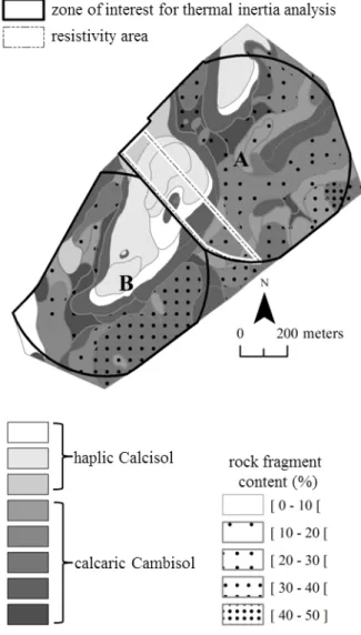
The study site was located in the Beauce region (France), on a cultivated field of 110 ha. About 300 auger holes were dug to characterize the soils (Fig-ure 1). The soils consisted of a loamy-clay layer de-veloped over the Beauce limestone bedrock or the cryoturbed or soft limestone deposits. They were haplic Calcisols or calcaric Cambisols (IUSS Work-ing Group WRB, 2006), and were classified into several soil units according to i) the bedrock where they have developed (cryoturbated or not), ii) the thickness of the loamy-clay layer (Figure 1), and iii) the volume proportion of rock fragments (Nicoullaud et al., 2004) (Figure 2). In the following, two spatial plots (plot A in the North-East and plot B in the South-West) will be considered in this study.
Figure 1. Localization of the auger holes and soil thickness measured at each auger hole. The lines delineate the soil types (see Figure 2)
Figure 2. Soil map of the studied area. The electrical resistivity area and the zone of interest for the thermal inertia analysis are delineated.
3.2 Electrical resistivity measurements
On a subplot of the plot A, electrical resistivity measurements were obtained at the field scale (see the location in Figure 2) by the use of the ARP© de-vice (Panissod et al., 1997), which is a mobile soil electrical resistivity mapping system, that comprises a multi-probe system of three arrays (V1, V2, V3 ar-rays) pulled by a cross-country vehicle. The distance between the current injection electrodes and meas-urement electrodes, and the distance between two electrodes for a given array are about 0.5 m for the V1 array, about 1 m for the V2 array and about 1.7 m for the V3 array. A resistivity meter injects 10 mA at 122 Hz and it is associated to a Doppler radar which triggers a measurement every 0.1 m along the electrical transect. The electrical measurements then consist of apparent resistivity measurements for three pseudo-depths. All the measurements were georeferenced and recorded on a PC. The electrical resistivity measurements with the ARP© device were recorded in August 2012, during summer, after harvest.
3.3 Airborne thermal inertia measurements
The thermal measurements were recorded by an ARIES radiometer that includes two numerical channels, one in the visible and near infra-red range (0.5-1 µm) and one in the thermal infra-red range (10.5-12.5µm) (Monge & Siriou, 1975). Two inter-nal blackbodies allow translating the recorded video signal in brightness temperature. The data acquisi-tion took place on December 11, 2002 at 10h 40 U.T. with a flight altitude of 1006 m, an ‘Instantane-ous Field Of View’ of 2.82 m at nadir. As demon-strated by Tabbagh (1977), morning flights are ad-vised, since superficial effects due to diurnal flux variations are minimized. The sampling step along a line was equal to 1.75 m. The mirror rotated at 36.4 Hz and the speed of the plane was 56.6 m.s-1. The data were corrected for pitch and roll using data from the gyroscope. After the flight, the anamorphic distortion was corrected and a last geometric rectifi-cation was done in the GIS.
By using the algorithm described in Scollar et al. (1990), the heat flux variations at the soil surface were calculated from the soil temperature data rec-orded between the 15th November 2002 and the 15th December 2002 at the nearby Bricy meteorological station at 10, 20, 50 and 100 cm depth. The cooling of the soil was significant during this period, espe-cially in the six days preceding the flight. The depth of investigation can thus be considering as greater than the thickness of the ploughed layer and we as-sume that the surface temperature reflect the thermal inertia of the subsoil. The video values were trans-lated in terms of apparent thermal inertia values of the soil horizon below the topsoil by assuming a 1.2 W m-1K-1 conductivity, a 0.48 m2s-1 diffusivity (1732 S.I. thermal inertia) and a 25 thickness for the top ploughed layer. On December 2002, the plot A exhibited bare soils, whereas residuals of vegetal straws covered the soils in plot B.
3.4 Comparison between airborne thermal inertia measurements, electrical resistivity
measurements and auger holes data.
A spatial correlation analysis was computed to compare apparent thermal inertia measurements and apparent electrical resistivity measurements on the subplot of the plot A.
On each parcel of the study area, a principal com-ponent analysis was conducted to define the pedo-logical characteristics that would be the most influ-ent on the airborne thermal inertial measureminflu-ents. To deal with the very local measurements on the au-ger holes compared to the resolution of the thermal inertia map, we have determined the median value of thermal inertia over a 5 m circle area, centered at the position of each auger hole.
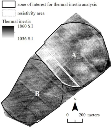
Figure 3. Apparent thermal inertia of the subsoil layer deduced from brightness temperature in the 10.5 – 12.5 µm channel.
4 RESULTS
4.1 The thermal inertia map
The thermal inertia map derived from the air-borne measurements on December 11th 2002 demon-strates that it varies from 1036 to 1860 S.I. over the studied area (Figure 3). It also exhibits a spatial or-ganization, with higher values in the plot B than in the plot A. In the plot B, linear structures that could be of anthropic origin, can be observed. On the con-trary, in the plot A, the structure of the signal does not resemble to regular structures and could be relat-ed to natural structures linkrelat-ed to the soil organiza-tion.
4.2 Comparison with the electrical resistivity measurements and discussion about the investigation depth
The electrical resistivity measurements were record-ed on a subplot of the plot A (Figure 4). The three arrays exhibited a similar spatial organization, with higher values in the South-East part and lower val-ues in the North-West part. As expected, they were strongly correlated (Table 1).
Table 1. Pearson correlation coefficients between the three ar-rays of electrical resistivity and the thermal inertia measure-ments.
Figure 4. Electrical resistivity maps for the V1, V2 and V3 ar-rays on the subplot of the parcel A. Comparison with the ther-mal inertia measurements in the same area.
The thermal inertia map showed a similar spatial or-ganization, with higher values in the South-East part and lower values in the North-West part. The corre-lation between thermal inertia measurements and electrical resistivity was higher with the V3 array (Table 1). Both electrical resistivity measurements and thermal inertia measurements were thus sensi-tive to the same pedological characteristics. The higher correlation with the V3 array suggests that the depth of investigation of the airbone thermal
meas-urements could be the same as the V3 array, say of about 1.70 m.
4.3 Influence of pedological data and soil types on the airborne thermal measurements
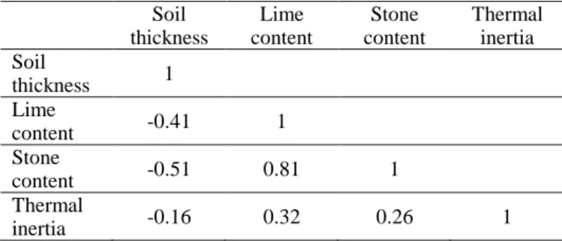
As airborne thermal inertia measurements seem to be better correlated to the V3 array and would thus ex-plore about 1.7 m depth, we have analyzed the rela-tionships between, on the one hand, the thermal iner-tia measurements, and on the other hand, the soil depth, the soil lime content, and the rock fragments contents because they are highly variable over the whole soil thickness in the studied area. On the plot A, with bare soils, the principal component analysis demonstrated that the thermal inertia was well-correlated to the soil thickness, the rock fragment content and the lime content with equivalent correla-tion coefficients (Figure 5, Table 2). Despite being significant also, the correlations coefficient were lower significant for the plot B, whose soils were partly covered by vegetal straws, especially as far as soil thickness is concerned (Figure 6, Table 3). In the PCA analysis, the thermal inertia was indeed associ-ated to the F2 axis, whereas the pedological charac-teristics were associated to the F1 axis.
Table 2. Pearson correlation coefficients between some pedo-logical characteristics and the thermal inertia measurements for the plot A. (number of observations: 159).
Soil thickness Lime content Stone content Thermal inertia Soil thickness 1 Lime content -0.28 1 Stone content -0.43 0.69 1 Thermal inertia -0.50 0.50 0.50 1
Table 3. Pearson correlation coefficients between some pedo-logical characteristics and the thermal inertia measurements for the plot B. (number of observations: 105).
Soil thickness Lime content Stone content Thermal inertia Soil thickness 1 Lime content -0.41 1 Stone content -0.51 0.81 1 Thermal inertia -0.16 0.32 0.26 1 Thermal inertia
V1 array V2 array V3 array Thermal inertia 1 V1 array 0.57 1 V2 array 0.65 0.91 1 V3 array 0.66 0.77 0.92 1
Figure 5. Principal component analysis with the airborne ther-mal inertia data and some pedological characteristics for the plot A.
Figure 6. Principal component analysis with the airborne ther-mal inertia data and some pedological characteristics for the plot A.
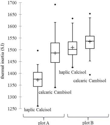
A statistical analysis was then conducted on the thermal inertia values on the two main soil types, say the Calcisols and the Cambisols (Figure 7). It demonstrated that, for the plot A the haplic Cal-cisols, that were calcareous, deep and contained only a small quantity of rock fragments, had thermal iner-tia values significantly different than the values for the calcaric Cambisols, that were thinner and con-tained significant quantities of rock fragments. For the plot B, the differences between the thermal iner-tia values between the Calcisols and the Cambisols
Figure 7. Comparison between the airborne thermal inertia data and the two soil types on the studied area for both the plots A and B.
were lower but remained significant. We can then conclude that the thermal inertia measurements seem to be efficient to discriminate between soil types, when the thermal prospection has been conducted on bare soils.
5 CONCLUSION
In this study case in the Beauce area, airborne ther-mal inertia mapping has demonstrated its ability to evidence the difference between two types of soils, that exhibit differences in soil stone content, lime content, soil thickness and degree of weathering of the calcareous on which soil have developed. In this study area, thermal inertia measurements and electri-cal resistivity measurements with an inter-electrode spacing of 1.70 m were influenced by the same pe-dological characteristics, and it appears as believable that the depth of investigation obtained for the De-cember 2002 airborne thermal inertia experiment was comparable with the one of the V3 array of the ARP© multi-depth system. Investigations have then to be continued to i) generalize these results to other contexts and ii) identify the optimum soil conditions to realize an airborne thermal inertia measurements campaign. The prospections should indeed be con-ducted when soil has been cooled (or warmed) for several days before the prospection, and when soils are not cover by straws. Despite these limitations, due to the spatial resolution of the measurement - of the order of 2 meters - and the possibility to cover
large areas of several square kilometers, airborne thermal inertia measurements appear as a promising tool to help in delineating soil characteristics and soil types in the Global Soil Map context.
REFERENCES
IUSS Working Group WRB. 2006. World reference base for
soil resources 2006. World Soil Resources Reports No.
103. FAO, Rome.
Monge, J.L. & Siriou, R. 1975. ARIES: un radiomètre multica-nal à balayage. 5th Spatial Optics meeting, Société Fran-çaise d’Optique, Marseille, June 1975, library of L.M.D, Ecole polytechnique, 91128 Palaiseau, France, 14 pp. Nicoullaud, B., Couturier, A., Beaudoin, N., Mary, B.,
Cou-tadeur, C. & King, D. 2004. Modélisation spatiale à l'échelle parcellaire des effets de la variabilité des sols et des pratiques culturales sur la pollution nitrique agricole. In:
Organisation spatiale des activités agricoles et processus environnementaux. P. Monestiez, S. Lardon, B. Seguin
(eds). Coll. Science Update, INRA Editions: 143-161. Panissod, C., Dabas, M., Jolivet, A. & Tabbagh, A. 1997. A
novel mobile multipole system (MUCEP) for shallow (0-3m) geoelectrical investigation: the ‘Vol-de-canards’ array.
Geophysical Prospecting 45: 983–1002.
Price J. C., 1977. Thermal inertia mapping: a new view of the earth. Journal of Geophysical Research 82-18: 2582-2590. Scollar, I., Tabbagh, A., Hesse, A. & Herzog, I. 1990.
Ar-chaeological prospecting and remote sensing. Cambridge
University Press, 674p.
Tabbagh, A. 1977. Sur la détermination du moment de mesure favorable et l’interprétation des résultats en prospection thermique archéologique. Annales de Géophysique 33: 243-254.