Accelerated Stochastic Matrix Inversion: General Theory and Speeding up BFGS Rules for Faster Second-Order Optimization

HAL Id: hal-02365327

https://hal.telecom-paris.fr/hal-02365327

Submitted on 15 Nov 2019

HAL is a multi-disciplinary open access

archive for the deposit and dissemination of

sci-entific research documents, whether they are

pub-lished or not. The documents may come from

teaching and research institutions in France or

abroad, or from public or private research centers.

L’archive ouverte pluridisciplinaire HAL, est

destinée au dépôt et à la diffusion de documents

scientifiques de niveau recherche, publiés ou non,

émanant des établissements d’enseignement et de

recherche français ou étrangers, des laboratoires

publics ou privés.

Accelerated Stochastic Matrix Inversion: General

Theory and Speeding up BFGS Rules for Faster

Second-Order Optimization

Robert Gower, Filip Hanzely, Peter Richtárik, Sebastian Stich

To cite this version:

Robert Gower, Filip Hanzely, Peter Richtárik, Sebastian Stich. Accelerated Stochastic Matrix

Inver-sion: General Theory and Speeding up BFGS Rules for Faster Second-Order Optimization.

Interna-tional Conference on Machine Learning, Jun 2019, Los Angeles, United States. �hal-02365327�

Accelerated Stochastic Matrix Inversion: General

Theory and Speeding up BFGS Rules for Faster

Second-Order Optimization

Peter Richtárik⇤ KAUST Thuwal, Saudi Arabia peter.richtarik@kaust.edu.sa Sebastian U. Stich EPFL Lausanne, Switzerland sebastian.stich@epfl.ch

Abstract

We present the first accelerated randomized algorithm for solving linear systems in Euclidean spaces. One essential problem of this type is the matrix inversion problem. In particular, our algorithm can be specialized to invert positive definite matrices in such a way that all iterates (approximate solutions) generated by the algorithm are positive definite matrices themselves. This opens the way for many applications in the field of optimization and machine learning. As an application of our general theory, we develop the first accelerated (deterministic and stochastic) quasi-Newton updates. Our updates lead to provably more aggressive approxima-tions of the inverse Hessian, and lead to speed-ups over classical non-accelerated rules in numerical experiments. Experiments with empirical risk minimization show that our rules can accelerate training of machine learning models.

1 Introduction

Consider the optimization problem

min

w2Rnf (w), (1)

and assume f is sufficiently smooth. A new wave of second order stochastic methods are being developed with the aim of solving large scale optimization problems. In particular, many of these new methods are based on stochastic BFGS updates [29, 35, 20, 21, 6, 8, 3]. Here we develop a new stochastic accelerated BFGS update that can form the basis of new stochastic quasi-Newton methods. Another approach to scaling up second order methods is to use randomized sketching to reduce the dimension, and hence the complexity of the Hessian and the updates involving the Hessian [26, 38], or subsampled Hessian matrices when the objective function is a sum of many loss functions [5, 2, 1, 37]. The starting point for developing second order methods is arguably Newton’s method, which performs the iterative process

wk+1= wk (_r2_{f (wk))} 1

rf(wk), (2)

where r2_{f (wk)and rf(wk)are the Hessian and gradient of f, respectively. However, it is inefficient} for solving large scale problems as it requires the computation of the Hessian and then solving a linear system at each iteration. Several methods have been developed to address this issue, based on the idea of approximating the exact update.

Quasi-Newton methods, in particular BFGS [4, 10, 11, 30], have been the leading optimization algorithm in various fields since the late 60’s until the rise of big data, which brought a need for simpler first order algorithms. It is well known that Nesterov’s acceleration [22] is a reliable way to speed up first order methods. However until now, acceleration techniques have been applied exclusively to speeding up gradient updates. In this paper we present an accelerated BFGS algorithm, opening up new applications for acceleration. The acceleration in fact comes from an accelerated algorithm for inverting the Hessian matrix.

To be more specific, recall that quasi-Newton rules aim to maintain an estimate of the inverse Hessian Xk, adjusting it every iteration so that the inverse Hessian acts appropriately in a particular direction, while enforcing symmetry:

Xk(_rf(wk) _rf(wk 1)) = wk wk 1, Xk = Xk>. (3) A notable research direction is the development of stochastic quasi-Newton methods [15], where the estimated inverse is equal to the true inverse over a subspace:

Xk_r2_{f (wk)Sk = Sk, Xk = X}>

k, (4)

where Sk_{2 R}n⇥⌧_{is a randomly generated matrix.}

In fact, (4) can be seen as the so called sketch-and-project iteration for inverting r2_{f (wk). In this} paper we first develop the accelerated algorithm for inverting positive definite matrices. As a direct application, our algorithm can be used as a primitive in quasi-Newton methods which results in a novel accelerated (stochastic) quasi-Newton method of the type (4). In addition, our acceleration technique can also be incorporated in the classical (non stochastic) BFGS method. This results in the accelerated BFGS method. Whereas the matrix inversion contribution is accompanied by strong theoretical justifications, this does not apply to the latter. Rather, we verify the effectiveness of this new accelerated BFGS method through numerical experiments.

1.1 Sketch-and-project for linear systems

Our accelerated algorithm can be applied to more general tasks than only inverting matrices. In its most general form, it can be seen as an accelerated version of a sketch-and-project method in Euclidean spaces which we present now. Consider a linear system Ax = b such that b 2 Range (A). One step of the sketch-and-project algorithm reads as:

xk+1=argminxkxk xkB2 subject to Sk>Ax = Sk>b, (5) where kxk2

B=hBx, xi for some B 0and Skis a random sketching matrix sampled i.i.d at each iteration from a fixed distribution.

Randomized Kaczmarz [16, 33] was the first algorithm of this type. In [13], this sketch-and-project algorithm was analyzed in its full generality. Note that the dual problem of (5) takes the form of a quadratic minimization problem [14], and randomized methods such as coordinate descent [23, 36], random pursuit [31, 32] or stochastic dual ascent [14] can thus also be captured as special instances of this method. Richtárik and Takáˇc [28] adopt a new point of view through a theory of stochastic reformulations of linear systems. In addition, they consider the addition of a relaxation parameter, as well as mini-batch and accelerated variants. Acceleration was only achieved for the expected iterates, and not in the L2 sense as we do here. We refer to Richtárik and Takáˇc [28] for interpretation of sketch-and-project as stochastic gradient descent, stochastic Newton, stochastic proximal point method, and stochastic fixed point method.

Gower [15] observed that the procedure (5) can also be applied to find the inverse of a matrix. Assume the optimization variable itself is a matrix, x = X, b = I, the identity matrix, then sketch-and-project converges (under mild assumptions) to a solution of AX = I. Even the symmetry constraint X = X>can be incorporated into the sketch-and-project framework since it is a linear constraint. There has been recent development in speeding up the sketch-and-project method using the idea of Nesterov’s acceleration [22]. In [18] an accelerated Kaczmarz algorithm was presented for special

sketches of rank one. Arbitrary sketches of rank one where considered in [31], block sketches in [24] and recently, Tu and coathors [34] developed acceleration for special sketching matrices, assuming the matrix A is square. This assumption, along with any assumptions on A, was later dropped in [27]. Another notable way to accelerate the sketch-and-project algorithm is by using momentum or stochastic momentum [19].

We build on recent work of Richtárik and Takáˇc [27] and further extend their analysis by studying accelerated sketch-and-project in general Euclidean spaces. This allows us to deduce the result for matrix inversion as a special case. However, there is one additional caveat that has to be considered for the intended application in quasi-Newton methods: ideally, all iterates of the algorithm should be symmetric positive definite matrices. This is not the case in general, but we address this problem by constructing special sketch operators that preserve symmetry and positive definiteness.

2 Contributions

We now present our main contributions.

Accelerated Sketch and Project in Euclidean Spaces. We generalize the analysis of an accelerated version of the sketch-and-project algorithm [27] to linear operator systems in Euclidean spaces. We provide a self-contained convergence analysis, recovering the original results in a more general setting.

Faster Algorithms for Matrix Inversion. We develop an accelerated algorithm for inverting positive definite matrices. This algorithm can be seen as a special case of the accelerated sketch-and-project in Euclidean space, thus its convergence follows from the main theorem. However, we also provide a different formulation of the proof that is specialized to this setting. Similarly to [34], the performance of the algorithm depends on two parameters µ and ⌫ that capture spectral properties of the input matrix and the sketches that are used. Whilst for the non-accelerated sketch-and-project algorithm for matrix inversion [15] the knowledge of these parameters is not necessary, they need to be given as input to the accelerated scheme. When employed with the correct choice of parameters, the accelerated algorithm is always faster than the non-accelerated one. We also provide a theoretical rate for sub-optimal parameters µ, ⌫, and we perform numerical experiments to argue the choice of µ, ⌫in practice.

Randomized Accelerated Quasi-Newton. The proposed iterative algorithm for matrix inversion is designed in such a way that each iterate is a symmetric matrix. This means, we can use the generated approximate solutions as estimators for the inverse Hessian in quasi-Newton methods, which is a direct extension of stochastic quasi-Newton methods. To the best of our knowledge, this yields the first accelerated (stochastic) quasi-Newton method.

Accelerated Quasi-Newton. In the standard BFGS method the updates to the Hessian estimate are not chosen randomly, but deterministically. Based on the intuition gained from the accelerated random method, we propose an accelerated scheme for BFGS. The main idea is that we replace the random sketching of the Hessian with a deterministic update. The theoretical convergence rates do not transfer to this scheme, but we demonstrate by numerical experiments that it is possible to choose a parameter combination which yields a slightly faster convergence. We believe that the novel idea of accelerating BFGS update is extremely valuable, as until now, acceleration techniques were only considered to improve gradient updates.

2.1 Outline

Our accelerated sketch-and-project algorithm for solving linear systems in Euclidean spaces is developed and analyzed in Section 3, and is used later in Section 4 to analyze an accelerated sketch-and-project algorithm for matrix inversion. The accelerated sketch-sketch-and-project algorithm for matrix inversion is then used to accelerate the BFGS update, which in turn leads to the development of an accelerated BFGS optimization method. Lastly in Section 5, we perform numerical experiments to gain different insights into the newly developed methods. Proofs of all results and additional insights can be found in the appendix.

3 Accelerated Stochastic Algorithm for Matrix Inversion

In this section we propose an accelerated randomized algorithm to solve linear systems in Euclidean spaces. This is a very general problem class which comprises the matrix inversion problem as well. Thus, we will use the result of this section later to analyze our newly proposed matrix inversion algorithm, which we then use to estimate the inverse of the Hessian within a quasi-Newton method.2 Let X and Y be finite dimensional Euclidean spaces and let A : X 7! Y be a linear operator. Let L(_{X , Y) denote the space of linear operators that map from X to Y. Consider the linear system}

Ax = b, (6)

where x 2 X and b 2 Range (A) . Consequently there exists a solution to the equation (6). In particular, we aim to find the solution closest to a given initial point x02 X :

x⇤ def= arg min x2X 1

2kx x0k

2 _{subject to Ax = b. (7)} Using the pseudoinverse and Lemma 22 item vi, the solution to (7) is given by

x⇤= x0 _A†(_Ax0 b)2 x0+ Range (A⇤) , (8) where A†_{and A}⇤_{denote the pseudoinverse and the adjoint of A, respectively.}

3.1 The algorithm

Let Z be a Euclidean space and consider a random linear operator Sk 2 L(Y, Z) chosen from some distribution D over L(Y, Z) at iteration k. Our method is given in Algorithm 1, where Zk 2 L(X ) is a random linear operator given by the following compositions

Zk= Z(_Sk)def=A⇤Sk⇤(SkAA⇤Sk⇤)†SkA. (9) The updates of variables gkand xk+1on lines 8 and 9, respectively, correspond to what is known as the sketch-and-project update:

xk+1= arg min x2X 1

2kx yk_k2 _{subject to S}

kAx = Skb, (10) which can also be written as the following operation

xk+1 x⇤= (I Zk)(yk x⇤). (11) This follows from the fact that b 2 Range (A), together with item i of Lemma 22. Furthermore, note that the adjoint A⇤_{and the pseudoinverse in Algorithm 1 are taken with respect to the norm} in (7).

Algorithm 1 Accelerated Sketch-and-Project for solving (10) [27]

1: Parameters: µ, ⌫ > 0, D = distribution over random linear operators.

2: Choose x02 X and set v0= x0, = 1 pµ_⌫, = q 1 µ⌫, ↵ = 1 1+ ⌫. 3: for k = 0, 1, . . . do 4: yk = ↵vk+ (1 ↵)xk

5: Sample an independent copy Sk_{⇠ D}

6: gk=_A⇤_S⇤

k(SkAA⇤Sk⇤)†Sk(Ayk b) = Zk(yk x⇤)

7: xk+1= yk gk

8: vk+1= vk+ (1 )yk gk

9: end for

Algorithm 1 was first proposed and analyzed by Richtárik and Takáˇc [27] for the special case when X = Rn_{and Y = R}m_{. Our contribution here is in extending the algorithm and analysis to the more} abstract setting of Euclidean spaces. In addition, we provide some further extensions of this method in Sections D and E, allowing for a non-unit stepsize and variable ↵, respectively.

2_{Quasi-Newton methods do not compute an exact matrix inverse, rather, they only compute an incremental} update. Thus, it suffices to apply one step of our proposed scheme per iteration. This will be detailed in Section 4.

3.2 Key assumptions and quantities

Denote Z = Z(S) for S ⇠ D. Assume that the exactness property holds

Null (_{A) = Null (E [Z]) ;} (12) this is also equivalent to Range (A⇤_{) = Range (E [Z]). The exactness assumption is of key} importance in the sketch-and-project framework, and indeed it is not very strong. For example, it holds for the matrix inversion problem with every sketching strategy we consider. We further assume that A 6= 0 and E [Z] is finite. First we collect a few observation on the Z operator

Lemma 1. The Z operator (9) is a adjoint positive projection. Consequently E [Z] is a self-adjoint positive operator.

The two parameters that govern the acceleration are µdef= inf x2Range(A⇤) hE[Z]x,xi hx,xi , ⌫ def = sup x2Range(A⇤) hE[ZE[Z]†Z_]x,xi hE[Z]x,xi . (13) The supremum in the definition of ⌫ is well defined due to the exactness assumption together with A 6= 0.

Lemma 2. We have

1 _ ⌫ _ 1_µ = _{kE [Z]}†_k. (14) Moreover, if Range (A⇤_{) =X , we have}

Rank(A⇤₎

E[Rank(Z)]  ⌫. (15) 3.3 Convergence and change of the norm

For a positive self-adjoint G 2 L(X ) and x 2 X let kxkG def= p

hx, xiG def= p

hGx, xi. We now informally state the convergence rate of Algorithm 1. Theorem 3 generalizes the main theorem from [27] to linear systems in Euclidean spaces.

Theorem 3. Let xk, vkbe the random iterates of Algorithm 1. Then Ehkvk x⇤k2_E[Z]†+µ1kxk x⇤k 2i ⇣1 qµ_⌫⌘ k Ehkv0 x⇤k2_E[Z]†+µ1kx0 x⇤k 2i_. This theorem shows the accelerated Sketch-and-Project algorithm converges linearly with a rate of

1 pµ_⌫ ,which translates to a total of O(p⌫/µ log (1/✏))iterations to bring the given error in Theorem 3 below ✏ > 0. This is in contrast with the non-accelerated Sketch-and-Project algorithm which requires O((1/µ) log (1/✏)) iterations, as shown in [13] for solving linear systems. From (14), we have the bounds 1/pµ p⌫/µ_{ 1/µ. On one extreme, this inequality shows that the iteration} complexity of the accelerated algorithm is at least as good as its non-accelerated counterpart. On the other extreme, the accelerated algorithm might require as little as the square root of the number of iterations of its non-accelerated counterpart. Since the cost of a single iteration of the accelerated algorithm is of the same order as the non-accelerated algorithm, this theorem shows that acceleration can offer a significant speed-up, which is verified numerically in Section 5. It is also possible to get the convergence rate of accelerated sketch-and-project where projections are taken with respect to a different weighted norm. For technical details, see Section B.4 of the Appendix.

3.4 Coordinate sketches with convenient probabilities

Let us consider a simple example in the setting for Algorithm 1 where we can understand parameters µ, ⌫. In particular, consider a linear system Ax = b in Rn_{where A is symmetric positive definite.} Corollary 4. Choose B = A and S = eiwith probability proportional to Ai,i. Then

µ = min(A)

Tr(A) =: µ

P _{and ⌫ =} Tr(A) miniAi,i =: ⌫

P ₍₁₆₎

and therefore the convergence rate given in Theorem 3 for the accelerated algorithm is ✓ 1 qµ_⌫ ◆k = ✓ 1 p

min(A) miniAi,i

Tr(A)

◆k

Rate (17) of our accelerated method is to be contrasted with the rate of the non-accelerated method: (1 µ)k _{= (1 min(A)/Tr (A)))}k_{.Clearly, we gain from acceleration if the smallest diagonal}

element of A is significantly larger than the smallest eigenvalue.

In fact, parameters µP_{, ⌫}P _{above are the correct choice for the matrix inversion algorithm, when} symmetry is not enforced, as we shall see later. Unfortunately, we are not able to estimate the parameters while enforcing symmetry for different sketching strategies. We dedicate a section in numerical experiments to test, if the parameter selection (16) performs well under enforced symmetry and different sketching strategies, and also how one might safely choose µ, ⌫ in practice.

4 Accelerated Stochastic BFGS Update

The update of the inverse Hessian used in quasi-Newton methods (e.g., in BFGS) can be seen as a sketch-and-project update applied to the linear system AX = I, while X = X> _{is enforced,} and where A denotes and approximation of the Hessian. In this section, we present an accelerated version of these updates. We provide two different proofs: one based on Theorem 3 and one based on vectorization. By mimicking the updates of the accelerated stochastic BFGS method for inverting matrices, we determine a heuristic for accelerating the classic deterministic BFGS update. We then incorporate this acceleration into the classic BFGS optimization method and show that the resulting algorithm can offer a speed-up of the standard BFGS algorithm.

4.1 Accelerated matrix inversion

Consider the symmetric positive definite matrix A 2 Rn⇥n_{and the following projection problem} A 1= arg min

X kXk 2

F (A) subject to AX = I, X = X>, (18) where kXkF (A)def= Tr AX>AX =kA1/2XA1/2k2F.This projection problem can be cast as an instantiation of the general projection problem (7). Indeed, we need only note that the constraint in (18) is linear and equivalent to A(X)def=⇣_{X X}AX>

⌘ = (I

0) .The matrix inversion problem can be efficiently solved using sketch-and-project with a symmetric sketch [15]. The symmetric sketch is given by SkA(X) =

⇣_S>

kAX

X X> ⌘

,where Sk 2 Rn⇥⌧_{is a random matrix drawn from a distribution D} and ⌧ 2 N. The resulting sketch-and-project method is as follows

Xk+1= arg min

X kX Xkk 2

F (A) subject to Sk>AX = Sk>, X = X>, (19) the closed form solution of which is

Xk+1= Sk(S>kASk) 1Sk>+ I Sk(Sk>ASk) 1Sk>A Xk I ASk(Sk>ASk) 1Sk> . (20) By observing that (20) is the sketch-and-project algorithm applied to a linear operator equation, we have constructed an accelerated version in Algorithm 2. We can also apply Theorem 3 to prove that Algorithm 2 is indeed accelerated.

Theorem 5. Let Lk def₌

kVk A 1k2M+µ1kXk A 1

k2

F (A). The iterates of Algorithm 2 satisfy E [Lk+1]_⇣1 qµ_⌫⌘E [Lk] , (21) where kXk2 M = Tr ⇣ A1/2_X>_A1/2_{E [Z]}†_A1/2_XA1/2⌘_{.Furthermore,} µdef= inf X2Rn⇥n hE[Z]X,Xi hX,Xi = min(E [Z]), ⌫ def = sup X2Rn⇥n

hE[ZE[Z]†Z]X,Xi

hE[Z]X,Xi , (22) where

Zdef= I_{⌦ I} (I P )_{⌦ (I} P ), P def= A1/2S(S>AS) 1S>A1/2, (23) and Z : X 2 Rn⇥n_{! R}n⇥n_{is given by Z(X) = X (I P ) X (I P ) = XP + P X(I P ).} Moreover, 2 min(E [P ]) min(E [Z]) min(E [P ]).

Notice that preserving symmetry yields µ = min(E [Z]), which can be up to twice as large as min(E [P ]), which is the value of the µ parameter of the method without preserving symmetry. This improved rate is new, and was not present in the algorithm’s debut publication [15]. In terms of parameter estimation, once symmetry is not preserved, we fall back onto the setting from Section 3.4. Unfortunately, we were not able to quantify the effect of enforcing symmetry on the parameter ⌫.

Algorithm 2 Accelerated BFGS matrix inversion (solving (18))

1: Parameters: µ, ⌫ > 0, D = distribution over random linear operators.

2: Choose X02 X and set V0= X0, = 1 pµ_⌫, = q 1 µ⌫, ↵ = 1 1+ ⌫ 3: for k = 0, 1, . . . do 4: Yk = ↵Vk+ (1 ↵)Xk

5: _{Sample an independent copy S ⇠ D}

6: Xk+1= Yk+ (YkA I)S(S>AS) 1_S> _S(S>_AS) 1_S>_AYk

7: +S(S>_AS) 1_S>_AYkAS(S>_AS) 1_S>

8: Vk+1= Vk+ (1 )Yk (Yk Xk+1)

9: end for

4.2 Vectorizing—a different insight

In the previous section we argued that Theorem 5 follows from the more general convergence result established in Theorem 3 for Euclidean spaces. We now show an alternative way to prove Theorem 5. Define Vec : Rn⇥n _{! R}n2 _{to be a vectorization operator of column-wise stacking and denote} xdef= Vec (X). It can be shown that the sketch-and-project operation for matrix inversion (4.2) is equivalent to

xk+1= arg min

x kx xkk 2

A⌦A subject to (I ⌦ Sk>)(I⌦ A)x = (I ⌦ Sk>)Vec (I) , Cx = 0, where C is defined so that Cx = 0 if and only if X = X>_{. The above is a sketch-and-project} update for a linear system in Rn2

, which allows to obtain an alternative proof of Theorem 5, without using our results from Euclidean spaces. The details are provided in Section H.2 of the Appendix. 4.3 Accelerated BFGS as an optimization algorithm

As a tweak in the stochastic BFGS allows for a faster estimation of Hessian inverse and therefore more accurate steps of the method, one might wonder if a equivalent tweak might speed up the standard, deterministic BFGS algorithm for solving (1). The mentioned tweaked version of standard BFGS is proposed as Algorithm 3. We do not state a convergence theorem for this algorithm—due to the deterministic updates the analysis is currently elusive—nor propose to use it as a default solver, but we rather introduce it as a novel idea for accelerating optimization algorithms. We leave theoretical analysis for the future work. For now, we perform several numerical experiments, in order to understand the potential and limitations of this new method.

Algorithm 3 BFGS method with accelerated BFGS update for solving (1)

1: Parameters: µ, ⌫ > 0, stepsize ⌘.

2: Choose X02 X , w0and set V0= X0, = 1 pµ_⌫, = q 1 µ⌫, ↵ = 1 1+ ⌫. 3: for k = 0, 1, . . . do 4: wk+1= wk ⌘Xk_rf(wk) 5: sk= wk+1 wk, ⇣k=_rf(wk+1) _rf(wk) 6: Yk = ↵Vk+ (1 ↵)Xk 7: Xk+1= k >k > k⇣k + ⇣ I k⇣k> > k⇣k ⌘ Yk⇣I ⇣k >k > k⇣k ⌘ 8: Vk+1= Vk+ (1 )Yk (Yk Xk+1) 9: end for

To better understand Algorithm 3, recall that the BFGS updates an estimate of the inverse Hessian via Xk+1=argminXkX Xkk2F (A) subject to X⇣k= k, X = X>, (24) where k = wk+1 wkand ⇣k=rf(wk+1) rf(wk). The above has the following closed form solution Xk+1= kk> > k⇣k+ ⇣ I k⇣>k > k⇣k ⌘ Xk⇣I ⇣k >k > k⇣k ⌘

.This update appears on line 7 of Algorithm 3 with the difference being that it is applied to a matrix Yk.

5 Numerical Experiments

We perform extensive numerical experiments to bring additional insight to both the performance of and to parameter selection for Algorithms 2 and 3. More numerical experiments can be found in Section A of the appendix. We first test our accelerated matrix inversion algorithm, and subsequently perform experiments related to Section 4.3.

5.1 Accelerated Matrix Inversion

We consider the problem of inverting a symmetric positive matrix A. We focus on a few particular choices of matrices A (specified when describing each experiment), that differ in their eigenvalue spectra. Three different sketching strategies are studied: Coordinate sketches with convenient probabilities (S = ei with probability proportional to Ai,i), coordinate sketches with uniform probabilities (S = eiwith probability 1

n) and Gaussian sketches (S ⇠ N (0, I)). As matrices to be inverted, we use both artificially generated matrices with the access to the spectrum and also Hessians of ridge regression problems from LIBSVM.

We have shown earlier that µ, ⌫ can be estimated as per (16) for coordinate sketches with convenient probabilities without enforcing symmetry. We use the mentioned parameters for the other sketching strategies while enforcing the symmetry. Since in practice one might not have an access to the exact parameters µ, ⌫ for given sketching strategy, we test sensitivity of the algorithm to parameter choice . We also test test for ⌫ chosen by (16), µ = 1

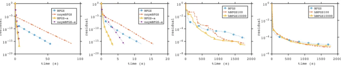
100⌫ and µ = 1 10000⌫. 0 50 100 time (s) 10-20 10-15 10-10 10-5 100 residual BFGS nsymBFGS BFGS-a nsymBFGS-a 0 5 10 15 20 time (s) 10-20 10-15 10-10 10-5 100 residual BFGS nsymBFGS BFGS-a nsymBFGS-a 0 500 1000 1500 2000 time (s) 10-8 10-6 10-4 10-2 100 residual BFGS hBFGS100 hBFGS10000 0 500 1000 1500 2000 time (s) 10-6 10-4 10-2 100 residual BFGS hBFGS100 hBFGS10000

Figure 1:From left to right: (i) Eigenvalues of A 2 R100⇥100_{are 1, 10}3_{, 10}3_{, . . . , 10}3_{and coordinate sketches} with convenient probabilities are used. (ii) Eigenvalues of A 2 R100⇥100_{are 1, 2, . . . , n and Gaussian sketches} are used. Label “nsym” indicates non-enforcing symmetry and “-a” indicates acceleration. (iii) Epsilon dataset (n = 2000), coordinate sketches with uniform probabilities. (iv) SVHN dataset (n = 3072), coordinate sketches with convenient probabilities. Label “h” indicates that minwas not precomputed, but µ was chosen as described in the text.

For more plots, see Section A in the appendix as here we provide only a tiny fraction of all plots. The experiments suggest that once the parameters µ, ⌫ are estimated exactly, we get a speedup comparing to the nonaccelerated method; and the amount of speedup depends on the structure of A and the sketching strategy. We observe from Figure 1 that we gain a great speedup for ill conditioned problems once the eigenvalues are concentrated around the largest eigenvalue. We also observe from Figure 1 that enforcing symmetry combines well with µ, ⌫ computed by (16), which does not consider the symmetry. On top of that, choice of µ, ⌫ per (16) seems to be robust to different sketching strategies, and in worst case performs as fast as the nonaccelerated algorithm.

5.2 BFGS Optimization Method

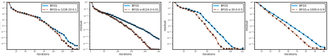
We test Algorithm 3 on several logistic regression problems using data from LIBSVM [7]. In all our tests we centered and normalized the data, included a bias term (a linear intercept), and choose the regularization parameter as = 1/m, where m is the number of data points. To keep things as simple as possible, we also used a fixed stepsize which was determined using grid search. Since our theory regarding the choice for the parameters µ and ⌫ does not apply in this setting, we simply probed the space of parameters manually and reported the best found result, see Figure 2. In the legend we use BFGS-a-µ-⌫ to denote the accelerated BFGS method (Alg 3) with parameters µ and ⌫. On all four datasets, our method outperforms the classic BFGS method, indicating that replacing classic BFGS update rules for learning the inverse Hessian by our new accelerated rules can be beneficial in practice. In A.4 in the appendix we also show the time plots for solving the problems in Figure 2, and show that the accelerated BFGS method also converges faster in time.

Figure 2: Algorithm 3 (BFGS with accelerated matrix inversion quasi-Newton update) vs standard BFGS. From left to right: phishing, mushrooms, australian and splice dataset.

6 Conclusions and Extensions

We developed an accelerated sketch-and-project method for solving linear systems in Euclidean spaces. The method was applied to invert positive definite matrices, while keeping their symmetric structure for all iterates. Our accelerated matrix inversion algorithm was then incorporated into an optimization framework to develop both accelerated stochastic and accelerated deterministic BFGS, which to the best of our knowledge, are the first accelerated quasi-Newton updates.

We show that under a careful choice of the parameters of the method—depending on the problem structure and conditioning—acceleration might result into significant speedups both for the matrix inversion problem and for the stochastic BFGS algorithm. We confirm experimentally that our accelerated methods can lead to speed-ups when compared to the classical BFGS algorithm. As a future line of research it might be interesting to study the accelerated BFGS algorithm (either deterministic or stochastic) further, and provide a convergence analysis on a suitable class of functions. Another interesting area of research might be to combine accelerated BFGS with limited memory [17] or engineer the method so that it can efficiently compete with first order algorithms for some empirical risk minimization problems, such as, for example [12].

As we show in this work, Nesterov’s acceleration can be applied to quasi-Newton updates. We believe this is a surprising fact, as quasi-Newton updates have not been understood as optimization algorithms, which prevented the idea of applying acceleration in this context.

Since since second-order methods are becoming more and more ubiquitous in machine learning and data science, we hope that our work will motivate further advances at the frontiers of big data optimization.

References

[1] Naman Agarwal, Brian Bullins, and Elad Hazan. Second-order stochastic optimization for machine learning in linear time. The Journal of Machine Learning Research, 18(1):4148–4187, 2017.

[2] Albert S Berahas, Raghu Bollapragada, and Jorge Nocedal. An investigation of Newton-sketch and subsampled Newton methods. CoRR, abs/1705.06211, 2017.

[3] Albert S Berahas, Jorge Nocedal, and pages=1055–1063 year=2016 Takáˇc, Martin, bookti-tle=Advances in Neural Information Processing Systems. A multi-batch l-bfgs method for machine learning.

[4] Charles G Broyden. Quasi-Newton methods and their application to function minimisation. Mathematics of Computation, 21(99):368–381, 1967.

[5] Richard H Byrd, Gillian M Chin, Will Neveitt, and Jorge Nocedal. On the use of stochastic hes-sian information in optimization methods for machine learning. SIAM Journal on Optimization, 21(3):977–995, 2011.

[6] Richard H Byrd, Samantha L Hansen, Jorge Nocedal, and Yoram Singer. A stochastic quasi-Newton method for large-scale optimization. SIAM Journal on Optimization, 26(2):1008–1031, 2016.

[7] Chih-Chung Chang and Chih-Jen Lin. Libsvm: A library for support vector machines. ACM Trans. Intell. Syst. Technol., 2(3):27:1–27:27, May 2011.

[8] Frank Curtis. A self-correcting variable-metric algorithm for stochastic optimization. In International Conference on Machine Learning, pages 632–641, 2016.

[9] Charles A Desoer and Barry H Whalen. A note on pseudoinverses. Journal of the Society of Industrial and Applied Mathematics, 11(2):442–447, 1963.

[10] Roger Fletcher. A new approach to variable metric algorithms. The computer journal, 13(3):317– 322, 1970.

[11] Donald Goldfarb. A family of variable-metric methods derived by variational means. Mathe-matics of computation, 24(109):23–26, 1970.

[12] Robert M Gower, Donald Goldfarb, and Peter Richtárik. Stochastic block BFGS: Squeezing more curvature out of data. In International Conference on Machine Learning, pages 1869–1878, 2016.

[13] Robert M Gower and Peter Richtárik. Randomized iterative methods for linear systems. SIAM Journal on Matrix Analysis and Applications, 36(4):1660–1690, 2015.

[14] Robert M Gower and Peter Richtárik. Stochastic dual ascent for solving linear systems. arXiv:1512.06890, 2015.

[15] Robert M Gower and Peter Richtárik. Randomized quasi-Newton updates are linearly convergent matrix inversion algorithms. SIAM Journal on Matrix Analysis and Applications, 38(4):1380– 1409, 2017.

[16] Stefan Kaczmarz. Angenäherte Auflösung von Systemen linearer Gleichungen. Bulletin International de l’Académie Polonaise des Sciences et des Lettres, 35:355–357, 1937.

[17] Dong C Liu and Jorge Nocedal. On the limited memory BFGS method for large scale optimiza-tion. Mathematical programming, 45(1-3):503–528, 1989.

[18] Ji Liu and Stephen J Wright. An accelerated randomized Kaczmarz algorithm. Math. Comput., 85(297):153–178, 2016.

[19] Nicolas Loizou and Peter Richtárik. Momentum and stochastic momentum for stochastic gradi-ent, Newton, proximal point and subspace descent methods. arXiv preprint arXiv:1712.09677, 2017.

[20] Aryan Mokhtari and Alejandro Ribeiro. Global convergence of online limited memory BFGS. The Journal of Machine Learning Research, 16:3151–3181, 2015.

[21] Philipp Moritz, Robert Nishihara, and Michael Jordan. A linearly-convergent stochastic L-BFGS algorithm. In Artificial Intelligence and Statistics, pages 249–258, 2016.

[22] Yurii Nesterov. A method of solving a convex programming problem with convergence rate O(1/k2_{). Soviet Mathematics Doklady, 27(2):372–376, 1983.}

[23] Yurii Nesterov. Efficiency of coordinate descent methods on huge-scale optimization problems. SIAM Journal on Optimization, 22(2):341–362, 2012.

[24] Yurii Nesterov and Sebastian U Stich. Efficiency of the accelerated coordinate descent method on structured optimization problems. SIAM Journal on Optimization, 27(1):110–123, 2017. [25] Gert K Pedersen. Analysis Now. Graduate Texts in Mathematics. Springer New York, 1996. [26] Mert Pilanci and Martin J Wainwright. Newton sketch: A near linear-time optimization

algorithm with linear-quadratic convergence. SIAM Journal on Optimization, 27(1):205–245, 2017.

[27] Peter Richtárik and Martin Takáˇc. Stochastic reformulations of linear systems: accelerated method. Manuscript, October 2017, 2017.

[28] Peter Richtárik and Martin Takáˇc. Stochastic reformulations of linear systems: algorithms and convergence theory. arXiv:1706.01108, 2017.

[29] Nicol N Schraudolph, Jin Yu, and Simon Günter. A stochastic quasi-Newton method for online convex optimization. In Artificial Intelligence and Statistics, pages 436–443, 2007.

[30] David F Shanno. Conditioning of quasi-Newton methods for function minimization. Mathemat-ics of computation, 24(111):647–656, 1970.

[31] Sebastian U Stich. Convex Optimization with Random Pursuit. PhD thesis, ETH Zurich, 2014. Diss., Eidgenössische Technische Hochschule ETH Zürich, Nr. 22111.

[32] Sebastian U Stich, Christian L Müller, and Bernd Gärtner. Variable metric random pursuit. Mathematical Programming, 156(1):549–579, Mar 2016.

[33] Thomas Strohmer and Roman Vershynin. A randomized Kaczmarz algorithm with exponential convergence. Journal of Fourier Analysis and Applications, 15(2):262, 2009.

[34] Stephen Tu, Shivaram Venkataraman, Ashia C Wilson, Alex Gittens, Michael I Jordan, and Benjamin Recht. Breaking locality accelerates block Gauss-Seidel. In Proceedings of the 34th International Conference on Machine Learning, ICML 2017, Sydney, NSW, Australia, 6-11 August 2017, pages 3482–3491, 2017.

[35] Xiao Wang, Shiqian Ma, Donald Goldfarb, and Wei Liu. Stochastic quasi-Newton methods for nonconvex stochastic optimization. SIAM Journal on Optimization, 27(2):927–956, 2017. [36] Stephen J Wright. Coordinate descent algorithms. Math. Program., 151(1):3–34, June 2015. [37] Peng Xu, Farbod Roosta-Khorasani, and Michael W Mahoney. Newton-type methods for

non-convex optimization under inexact hessian information. arXiv preprint arXiv:1708.07164, 2017.

[38] Peng Xu, Jiyan Yang, Farbod Roosta-Khorasani, Christopher Ré, and Michael W Mahoney. Sub-sampled newton methods with non-uniform sampling. In Advances in Neural Information Processing Systems, pages 3000–3008, 2016.