Adjoint error estimation for residual based discretizations of hyperbolic conservation laws I : linear problems
Texte intégral
Figure
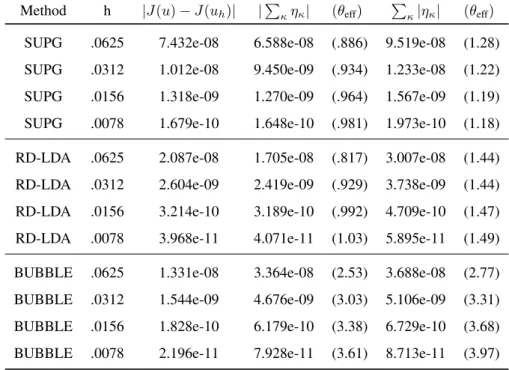
![Table 3: Efficiency rates p p = 1 and p a = 2 order of the SUPG, RD and BUBBLE methods error estimates : circular advection problem [6].](https://thumb-eu.123doks.com/thumbv2/123doknet/12420100.333682/16.892.151.661.223.591/table-efficiency-bubble-methods-estimates-circular-advection-problem.webp)
![Table 4: Efficiency rates primal p p = 2 and p a = 3 order of the SUPG, RD and BUBBLE methods error estimates : circular advection problem [6].](https://thumb-eu.123doks.com/thumbv2/123doknet/12420100.333682/17.892.227.737.222.594/table-efficiency-bubble-methods-estimates-circular-advection-problem.webp)


Documents relatifs
We prove higher regularity of the control and develop a priori error analysis for the finite element discretization of the shape optimization problem under consideration.. The derived
Comparison of the method with the results of a Gaussian kernel estimator with an unsymmetric noise (MISE × 100 averaged over 500 simulations), ˆ r ker is the risk of the
Anisotropic a posteriori error estimation for the mixed discontinuous Galerkin approximation of the Stokes problem... mixed discontinuous Galerkin approximation of the
• A posteriori error estimation tools used to compute the error • The computation of the bound is deterministic. • The second moment of the quantity of interest can be bounded –
We introduce a residual-based a posteriori error estimator for contact problems in two and three dimensional linear elasticity, discretized with linear and quadratic finite elements
Residual based error estimators seek the error by measuring, in each finite element, how far the numerical stress field is from equilibrium and, consequently, do not require
Polynomial robust stability analysis for H(div)-conforming finite elements for the Stokes equations. Elliptic reconstruction and a posteriori error estimates for parabolic
Thus, in [20] adjoint theory is employed to estimate the simplification error, which improves the error estimation results for internal and negative boundary features with Neumann
