HAL Id: hal-00639041
https://hal.inria.fr/hal-00639041
Submitted on 8 Nov 2011
HAL is a multi-disciplinary open access
archive for the deposit and dissemination of
sci-entific research documents, whether they are
pub-lished or not. The documents may come from
teaching and research institutions in France or
abroad, or from public or private research centers.
L’archive ouverte pluridisciplinaire HAL, est
destinée au dépôt et à la diffusion de documents
scientifiques de niveau recherche, publiés ou non,
émanant des établissements d’enseignement et de
recherche français ou étrangers, des laboratoires
publics ou privés.
A 64-Kbytes ITTAGE indirect branch predictor
André Seznec
To cite this version:
André Seznec. A 64-Kbytes ITTAGE indirect branch predictor. JWAC-2: Championship Branch
Prediction, JILP, Jun 2011, San Jose, United States. �hal-00639041�
A 64-Kbytes ITTAGE indirect branch predictor
∗
Andr´e Seznec
INRIA/IRISA
Abstract
The ITTAGE, Indirect Target TAgged GEometric length predictor, was introduced in [5] at the same time as the TAGE conditional branch predictor.
ITTAGE relies on the same principles as the TAGE predictor several predictor tables in-dexed through independent functions of the global branch/path history and the branch address. Like the TAGE predictor, ITTAGE uses (partially) tagged components as the PPM-like predictor [2]. It relies on (partial) match to select the predicted target of an indirect jump. TAGE also uses GEometric history length as the O-GEHL predictor [3], i.e. , the set of used global history lengths forms a geometric series. This allows to efficiently capture correlation on recent branch outcomes as well as on very old branches.
Due to the huge storage budget available for the ChampionShip, we propose an ITTAGE predictor fea-turing 16 prediction tables. On the distributed set of traces, using a path history vector recording only in-formation from indirect jumps and calls was found to be (slightly) more efficient than using a path/branch history vector combining information from all kind of branches.
1
The ITTAGE indirect jump target
predictor
Building on top of the cascaded predictor [1] and on the TAGE predictor, the ITTAGE predictor was proposed in [4]. In this section, we recall the gen-eral principles of the ITTAGE indirect target pre-dictor.equivalent storage budget. Some implementa-tion details from the initial ITTAGE proposiimplementa-tion are slightly modified in order to improve the global pre-diction accuracy.
1.1
ITTAGE predictor principles
ITTAGE relies on the same principles as the TAGE predictor several predictor tables indexed through in-dependent functions of the global branch/path his-tory and the branch address.
∗This work was partially supported by the European Re-search Counsil Advanced Grant DAL
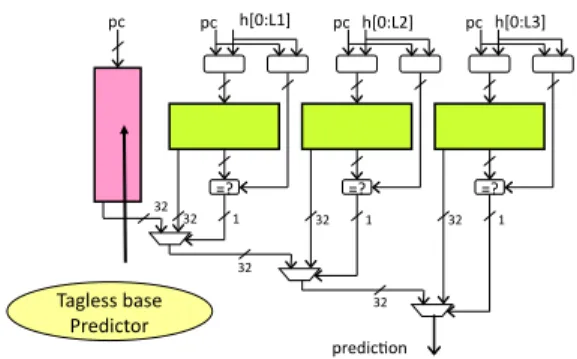
The Indirect Target TAgged GEometric length, ITTAGE, predictor features a tagless base predic-tor T0 in charge of providing a default prediction and a set of (partially) tagged predictor components. The tagged predictor components Ti, 1 ≤ i < M are indexed using different history lengths. The set of history lengths form an increasing series, i.e L(i) = (int)(αi−1∗ L(1) + 0.5). This is illustrated
in Figure 1. The counters representing predictions in TAGE are replaced by the target addresses Target . A predictor table entry also features a tag, a 2-bit confidence counter Ctr allowing some hysteresis on the predictor and a useful bit U for controlling the update policy ( Figure 2).
pc h[0:L1] =? =? =? predic1on pc pc h[0:L2] pc h[0:L3] 32 32 1 32 1 32 1 32 32 Tagless base Predictor
Figure 1: The Indirect Target TAgged GEometric length, ITTAGE, predictor
Target Tag Ctr U
Figure 2: An entry of an ITTAGE predictor table
A few definitions and notations In the remain-der of the paper, we define the proviremain-der component as the predictor component that ultimately provides the prediction. We define the alternate prediction altpred as the prediction that would have occurred if there had been a miss on the provider component. That is, if there are tag hits on T2 and T4 and tag misses on T1 and T3, T4 is the provider component
and T2 provides altpred. If there is no hitting com-ponent then altpred is the default prediction.
1.1.1 Prediction computation
The prediction selection algorithm is directly inher-ited from the TAGE predictor [4]. The optimization for weak counters entries proposed for TAGE (Sec-tion 3.2.4 [4]) is also implemented.
At prediction time, the base predictor and the tagged components are accessed simultaneously. The prediction is provided by the hitting tagged predictor component that uses the longest history. In case of no matching tagged predictor component, the default prediction is used.
The optimization for weak confidence counters We remarked that when the confidence counter of the matching entry is null, on some traces, the alternate prediction altpred is sometimes more accurate than the ”normal” prediction. This property is global to the application and can be dynamically monitored through a single 4-bit counter (USE ALT ON NA in the simulator). On the distributed benchmark set, this optimization reduces the misprediction number by 2%.
Prediction computation summary Therefore the prediction computation algorithm is as follows:
1. Find the longest matching component and the alternate component
2. if (the confidence counter is non-null or USE ALT ON NA is negative) then the provider component provides the prediction else the pre-diction is provided by the alternate component
1.1.2 Updating the ITTAGE predictor Update on a correct prediction The confidence counter of the provider component is incremented. Update on a misprediction First we update the provider component entry. If the confidence counter is non-null then we decrement it. If the confidence counter is null then we replace the Target field in the predictor entry by the effective target of the branch. As a second step, if the provider component Ti is not the component using the longest history (i.e., i < M) , we try to allocate entries on predictor components Tk using a longer history than Ti (i.e., i < k < M). Since, the predictor size storage bud-get allocated for the competition is huge we allocate up to 3 of these entries. For smaller predictors, one would try to limit the footprint of the application on the predictor by allocating a single predictor entry.
The M-i-1 uj useful bits are read from predictor
components Tj, i < j < M . The allocation algo-rithm chose up to four entries for which the useful bits are null, moreover we guarantee that the entries are not allocated in consecutive tables. On an allo-cated entry, the confidence counter is set to weak and the useful bit is set to null.
Updating the useful bitu The useful bit u of the provider component is set whenever the actual pre-diction is correct and the alternate prepre-diction altpred is incorrect.
In order to avoid that useful bits stay forever set, we implement the following reset policy. On allo-cation of new entries, we dynamically monitor the number of successes and fails when trying to allocate new entries after a misprediction; this monitoring is performed through a single 8-bit counter (u=1, incre-ment, u=0 decrement). This counter (variable TICK in the simulator) saturates when more fails than suc-cesses are encountered on updates. At that time we reset all the u bits of the predictor. Typically, such a global reset occurs when in average half of the entries on the used portion of the predictor has been set to useful. This simple policy was found to be more ef-ficient than the previously proposed management for useful counters for the TAGE predictor [5][4].
2
A few optimizations
2.1
The global history vector
The combination of the global branch history vec-tor and a short path hisvec-tory (limited to 1 bit per branch) used in [5] was found to be significantly outperformed by a global history vector introducing much more information for the indirect branches as well as for the calls. Respectively 10 bits and 5 bits mixing target and program counter are introduced for the indirect branches and the calls. This reduces the misprediction number by nearly 16 % compared with using a single (taken/not taken) bit for each branch. Experiments showed that using only path informa-tions bits of indirect branches and calls results in bet-ter performance on the set of distributed traces than also incorporating information for the other branches. However drawing conclusions from this experi-ment appears as really hazardous as the perfor-mance difference with using a global history vector where other branches are inserted as a single bit is marginal (about 3,000 mispredictions in total over the 40 distributed traces). It should be pointed out that, for the submitted predictor, three single indi-rect branches constitute a very significant fraction of the mispredictions: two branches common to traces INT05 and INT06 (which are traces from the same
application) and aone branch from SERVER01. The two branches from INT05 and INT06 are better pre-dicted by the history vector combining only indirect branches and calls. Discounting INT05 and INT06 (or even only one of them) would have pushed to use the more conventional history including all branches.
2.2
Leveraging target locality
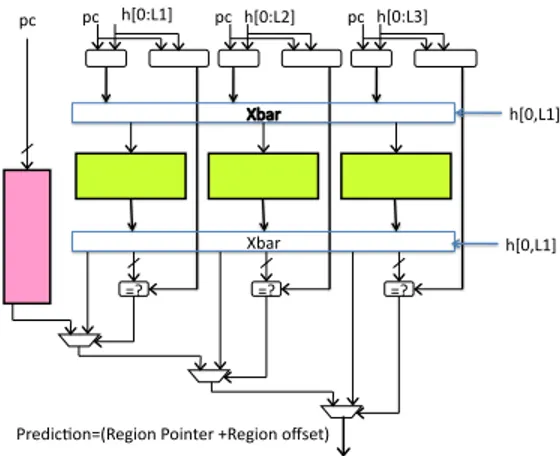
The target field represents the major storage cost in a predictor entry. However branch targets exhibit some address locality. Exploiting such locality is not that simple since some of the benchmarks use tar-gets scattered on more 1K 4Kbytes pages. However we found that all the benchmarks uses less than 128 256Kbytes. Therefore the Target field (32 bits) in a predictor entry is replaced by a Region offset (18 bits) and a Region pointer ( 7 bits), thus saving 7 bits on each entry (Figure 3). A 128-entry target region table must be added to rebuild the complete address, each entry featuring a 14-bit region address and a Useful bit for replacement. On a prediction, the target region table is only read at a given ad-dress. On a misprediction, the target region table is fully-associative searched for the matching region for the effective target; in case of a miss on the target region table, a target region entry is allocated.
The total storage for the target region table is 15*128 bits, i.e. 240 bytes. It should be noticed that
Target Tag Ctr U
Region offset Region pointer
Figure 3: Exploiting indirect target locality for 64-bit architecture the use of indirect access to target region table would allow to nearly halves the total storage size of the predictor.
2.3
Miscelleanous optimizations
We present here two optimizations that are pro-posed for the ISL-TAGE predictor for the companion conditional predictor contest. We have implemented them in the submitted predictor, but that do not bring very significant benefit: in total they reduce the misprediction number by less than 1 %.
2.3.1 Sharing storage space between predic-tor tables
As represented on Figure 1, ITTAGE predictor fea-tures independent tables. For some applications, some of the tables are underutilized while some others
are under large pressure. Sharing the storage space among several tables can be implemented without re-quiring to a real multiported memory table, but a bank interleaved table. E.g on Figure 4, T1. T2, and T3 are grouped in a 4-way interleaved table, history vector of length L(1) is hashed to determine the bank that will deliver prediction for T1, prediction for T2 is delivered by the adjacent bank , etc,.
pc =? =? =? Predic+on=(Region Pointer +Region offset) Xbar h[0:L1] pc pc h[0:L2] pc h[0:L3] h[0,L1] h[0,L1]
Figure 4: Sharing storage space between predictor tables
Experiments showed that global interleaving of all tables is not the best solution, but that interleaving between for a few adjacent history lengths can be beneficial. Groups T0 T1-T2 T3-T10 T11-T15 Total Entries 4K 4K 4K 2K 14 K Tag bits 0 9 13 15 U bit 0 1 1 1 bits/entry 27 37 41 43 Kbits 108 148 164 86 506
Table 1: Characteristics of the tables of the ITTAGE predictor
2.3.2 Dealing with delayed updates: The im-mediate update mimicker
On a real hardware processor, the predictor tables are updated at retire time to avoid pollution of the predictor by the wrong path. A single predictor table entry may provide several mispredictions in a row due to this late update. In order to reduce this impact, we implement an add-on to TAGE, the IUM, immediate update mimicker.
However on a misprediction the history can be re-paired immediately and when a block is fetched on the correct path, the still speculative branch history is correct. In practice, repairing the global history is straightforward if one uses a circular buffer to im-plement the global history. We leverage the same idea with IUM predictor. When fetching an indirect branch, IUM memorizes the identity of the entry E in the ITTAGE predictor (number of the table and its index) that provides the prediction as well as the predicted direction. At branch resolution on a mis-prediction, the IUM is repaired through reinitializing its head pointer to the associated IUM entry and up-dating this entry with the correct target.
When fetching on the correct path, the associated IUM entry associated with an inflight branch B fea-tures the matching predictor entry E that provided the ITTAGE prediction and the effective target of branch B (corrected in case of a misprediction on B). In case of a new hit on entry E in the predictor before the retirement of branch B, the (ITTAGE predictor + IUM) can respond with the direction provided by the IUM rather than with the ITTAGE prediction (on which entry E has not been updated).
IUM can be implemented in hardware through a fully-associative table, It allows to recover about 3/ 4th of the mispredictions due to late update of the IT-TAGE predictor tables. The storage cost of the spec-ulative predictor is only 64*48 bits, i.e. 384 bytes, plus the pointers to determine the head ( position of the last fetch branch) and the tail ( position of the next to be retired branch) of the IUM.
3
The submitted predictor
character-istics
The characteristics of the submitted are summa-rized in Table 1. Both Tables T0 and T1 are directly indexed with the program counter since some of the benchmarks feature a huge number of static indirect branches and it appeared that the performance of the predictor on those benchmarks might have been im-paired by conflicts on T0. T0 does not feature tags and u bits.
We have chosen a guided search of the best set of history lengths. Using a geometric series with min-imum history length 8 and maxmin-imum history length 2000, we first determined the number of tables (16), their grouping, their respective sizes and their tag widths. Table T0 is not shared. Tables T1 and T2 form a first sharing group. T3 to T10 form a second sharing group and T11 to T15 form the last group. The set of possible history lengths was then explored with the geometric series as the starting point. The
set of history lengths in the submitted predictor is {0, 0, 10, 16, 27, 44, 60, 96, 109, 219, 449, 487, 714, 1313, 2146, 3881}. These characteristics are summarized in Table 1.
The storage cost of the predictor consists in a total of 506Kbits of storage for the ITTAGE predictor ta-bles, 240 bytes for the target region table, 384 bytes for IUM, i.e. a total of 65,392 bytes of storage for predictions and target regions.
The storage needed for the extra logic consists of a circular buffer of for storing the history bits (for simplifying the code, we use a 4Kbits buffer), two 12-bit pointer on this buffer for respectively speculative history and retire history, a 32-bit register for pseudo-random value computed on the fly, a 8-bit counter to control the reset of the u bits, a 4-bit counter to control the possible use of the alternate prediction, two 6-bit pointers on the IUM i.e a total of 4176 bits of extra storage for the history and control logic.
4
Options of the submitted ITTAGE
predictor
Through commenting some #define lines, one can run different versions of the submitted predictor.
⁀#define IUM enables the IUM predictor.
#define INITHISTLENGTH enables the use of the best found set of history length.
#define SHARINGTABLES enables the sharing of storage tables among the logic tables of the ITTAGE predictor.
References
[1] K. Driesen and U. Holzle. The cascaded predictor: Economical and adaptive branch target prediction. In
Proceeding of the 30th Symposium on Microarchitec-ture, December 1998.
[2] Pierre Michaud. A ppm-like, tag-based pre-dictor. Journal of Instruction Level Parallelism (http://www.jilp.org/vol7), April 2005.
[3] A. Seznec. Analysis of the o-gehl branch predictor. In
Proceedings of the 32nd Annual International Sympo-sium on Computer Architecture, june 2005.
[4] Andr´e Seznec. The l-tage branch predic-tor. Journal of Instruction Level Parallelism (http://wwwjilp.org/vol9), April 2007.
[5] Andr´e Seznec and Pierre Michaud. A case for (partially)-tagged geometric history length predic-tors. Journal of Instruction Level Parallelism (http://www.jilp.org/vol8), April 2006.