HAL Id: hal-02888452
https://hal.archives-ouvertes.fr/hal-02888452
Submitted on 13 Jan 2021HAL is a multi-disciplinary open access
archive for the deposit and dissemination of sci-entific research documents, whether they are pub-lished or not. The documents may come from
L’archive ouverte pluridisciplinaire HAL, est destinée au dépôt et à la diffusion de documents scientifiques de niveau recherche, publiés ou non, émanant des établissements d’enseignement et de
Contextual classification for smart machining based on
unsupervised machine learning by Gaussian mixture
model
Zhiqiang Wang, Mathieu Ritou, Catherine da Cunha, Benoît Furet
To cite this version:
Zhiqiang Wang, Mathieu Ritou, Catherine da Cunha, Benoît Furet. Contextual classification for smart machining based on unsupervised machine learning by Gaussian mixture model. International Journal of Computer Integrated Manufacturing, Taylor & Francis, 2020, 33 (10-11), pp.1042-1054. �10.1080/0951192X.2020.1775302�. �hal-02888452�
Contextual classification for smart machining based on unsupervised machine learning by Gaussian mixture model
Zhiqiang Wanga,b, Mathieu Ritoua,b, Catherine Da Cunhaa,cand Benoˆıt Fureta,b
aLaboratory of digital sciences of Nantes (LS2N, UMR CNRS 6004), Nantes, France; bUniversity of Nantes, Nantes, France;cCentrale Nantes, Nantes, France
ABSTRACT
Intelligent machine-tools generate a large amount of digital data. Data mining can support decision making for operational management. The first step in a data min-ing approach is the selection of relevant data. Raw data must, therefore, be classified into different groups of contexts. This paper proposes an original contextual clas-sification of data for smart machining based on unsupervised machine learning by Gaussian mixture model. The optimal number of classes is determined by the silhou-ette method based on the Bayesian information criterion. This method is validated on real data from four different machine-tools in the aerospace industry. Manual data mining and k-fold cross validation confirm that the proposed method provides good contextual classification results. Then, several key performance indicators are calculated using this contextual classification. They show the relevancy of the ap-proach.
KEYWORDS
Industry 4.0, machining, unsupervised machine learning, GMM, BIC.
1. Introduction
High-Speed Machining (HSM) has significantly increased spindle speed compared to conventional machining. Production systems are very flexible, especially in the aero-nautics industry, where hundreds of tools machine several thousands of parts with different references on the same site. It is not easy for the Manufacturing Department to identify problematic programs or tools. The main problems are chatter (instabil-ity during machining), tool breakage and over-vibrations. Therefore, a data mining system is necessary to protect the machine-tool and work-pieces (especially for aero-nautical parts which present high value-added). Teti et al. (2010) make an overview of the existing techniques of machining monitoring and list all measurable and studied defects. Maleki et al. (2017) proposed a FMEA-based approach for the choice of the sensors. Quintana and Ciurana (2011) focus on the state of the art on chatter and existing methods to detect and to avoid it. Zhou and Xue (2018) make a summary of the methods used to monitor tool wear in milling processes, including sensors, feature extraction and monitoring models. Godreau et al. (2019) propose a vibration criterion for the detection of chatter, a source of non-quality.
In the general context of Industry 4.0, large volumes of manufacturing data are available on instrumented machine-tool. They are interesting to exploit not only to im-prove machine-tool performance but also to support the decision making of operational
CONTACT Mathieu Ritou. Email: [email protected]
Preprint of: Z. Wang, M. Ritou, C. da Cunha, B. Furet, Contextual classification for smart
machining based on unsupervised machine learning by Gaussian mixture model, International Journal of Computer Integrated Manufacturing, Vol. 33 n°10-11, p. 1042-1054, 2020.
management. Lenz, Wuest, and Westk¨amper (2018) propose a holistic approach to ma-chining data analysis in order to combine tasks and to group analysis objectives among different departments within the company. Morgan and ODonnell (2018) present the design and development of a cyber-physical process monitoring system for machine-tool. Liu et al. (2018) propose a systematic development method for machine-tool 4.0. In order to extract data from databases more efficiently and accurately, contextual classification is necessary to understand the status of the machine-tool and to real-ize a more relevant calculation of Key Performance Indicators (KPI). Many researches propose the use of machine learning algorithms directly on the raw data (machine-tool signals). However, few researches focus on data pre-processing to identify the context. In this article, machine learning algorithms for contextual classification are developed. They will permit a more relevant calculation of Key Performance Indicators.
Machine Learning is a field of Artificial Intelligence that relies on statistical ap-proaches. It can be applied to machine-tool signals analysis. Kim et al. (2018) list and summarize machining contributions using machine learning algorithms. There are two categories: supervised and unsupervised machine learning.
- Supervised machine learning learns to classify from already labeled output sam-ples. It aims at making correct predictions on the data which is not present in the learning set. For example, El-Mounayri and Deng (2010) designed and im-plemented a neural networks (ANN) for force prediction to optimize the cutting parameters in optimizing 21/2- axis milling; C. Zhang and H. Zhang (2016) show
that the least squares support vector machine (SVM)-based tool wear model is suitable to predict tool wear at certain range of cutting conditions in milling op-eration; Rodr´ıguez et al. (2017) propose a decision-making tool based on decision trees for roughness prediction in face milling.
- Unsupervised machine learning learns to classify unlabeled data. There are dif-ferent types of unsupervised learning: K-means, hierarchical classification (as-cending or des(as-cending), distribution density estimates (e.g., Gaussian Mixing Model - GMM). Bhinge et al. (2014) build an energy prediction model when machining a component using the Gaussian regression algorithm. Godreau et al. (2019) calculate the criteria thresholds by applying the Maximum Likelihood Estimation method.
In industry, it is challenging to collect labeled output data. As a result, most in-dustrial applications use unsupervised machine learning methods. In a previous study, Wang et al. (2019) compared the different methods of unsupervised machine-learning, and Gaussian Mixture Model (GMM) was the most effective for contextual classifi-cation. Another challenge of smart-machining comes from the management of time series; the state of the machine can change whenever and has to be identified every tenth of a second.
In this article, unsupervised machine learning by Gaussian Mixture Model (GMM) is used. GMM is a statistical tool used to parametrically estimate the distribution of random variables by modeling them as a mixture of Gaussian distributions (Reynolds 2015). The distributions’ parameters are estimated from the learning data using the Maximization Expectation algorithm. The main advantage of GMM is that it can cor-rectly classify data with unbalanced classes, while its disadvantage is that the results of GMM directly depend on the choice of parameters. An additional algorithm can there-fore be useful to determine the necessary number of classes automatically (Schwarz et al. 1978). The Bayesian Information Criterion (BIC) is particularly recommended. This paper proposes an original contextual classification of data for smart machining
based on unsupervised machine learning by Gaussian mixture model. The method is applied to four machining databases collected in the aeronautics industry. The number of classes is determined by the BIC method. The classifications are then evaluated using manual data mining and k-fold validation. This paper is organized as follows. Section 2 introduces the framework of the study as well as the contextual classification method. Section 3 proposes the method based on Gaussian Mixture Model (GMM). The next section depicts the silhouette method, which determines the optimal number of classes. Section 5 applies the proposed method to vibration signals and power signals to know whether the tool is cutting materials or not. Section 6 verifies the obtained classification using manual data mining and k-fold cross-validation. Section 7 presents KPIs based on the obtained contextual classification. These indicators will aid decision-making within the company.
2. Data analysis process 2.1. Framework of the study
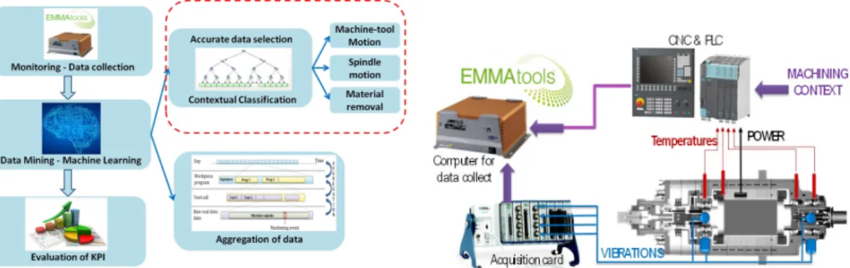
The work presented in this article is a part of the ANR SmartEmma project, which aims at developing intelligent and connected machine-tools. Fig. 1(a) shows an overview of the road-map of this project. A device, called Emmatools, collects the measured data during machining and stores it in a database (De Castelbajac et al. 2014). It is installed on machine-tools in factories of aircraft manufacturers. Fig. 1(b) presents the schematic diagram of the Emmatools. It collects data every tenth of a second. The data comes from two information sources: the Computer Numerical Con-trol (CNC) and the added sensors. By field bus, the CNC provides machining context data such as the tool name, the current program, machine, and spindle motions. The sensors integrated into the machine-tool collect the instantaneous power of the spin-dle, temperatures, as well as the vibrations from 4 accelerometers integrated into the spindle (radially at each bearing).
Figure 1. Data mining process for machining (a) and schematic diagram of the data collect device (b)
The machine learning methods will be developed on the one hand to perform con-textual classifications, and on the other, to aggregate the data. The latter concept can be found in Ritou et al. (2019), which proposes a method to address the issue of data volume using multi-level aggregation. 1 GB of data is collected per day and per machine-tool. Contextual classification permits to classify raw data into ordered and meaningful forms. Using this contextual information, noise is reduced and relevant KPIs can be calculated. Those KPIs support decisions on the HSM process and the
global management of the company.
2.2. Contextual classification method
As previously mentioned, contextual classification enables a more relevant evaluation of KPIs. In the context of our research work, it is interesting to know:
- if the spindle is stopped (S) or rotating at constant speed (CS) or varying speed (VS);
- if the machine-tool is stopped or moving at constant or varying speed;
- if the tool is cutting materials or not (N), with a constant (CC) or varying tool engagement (CV).
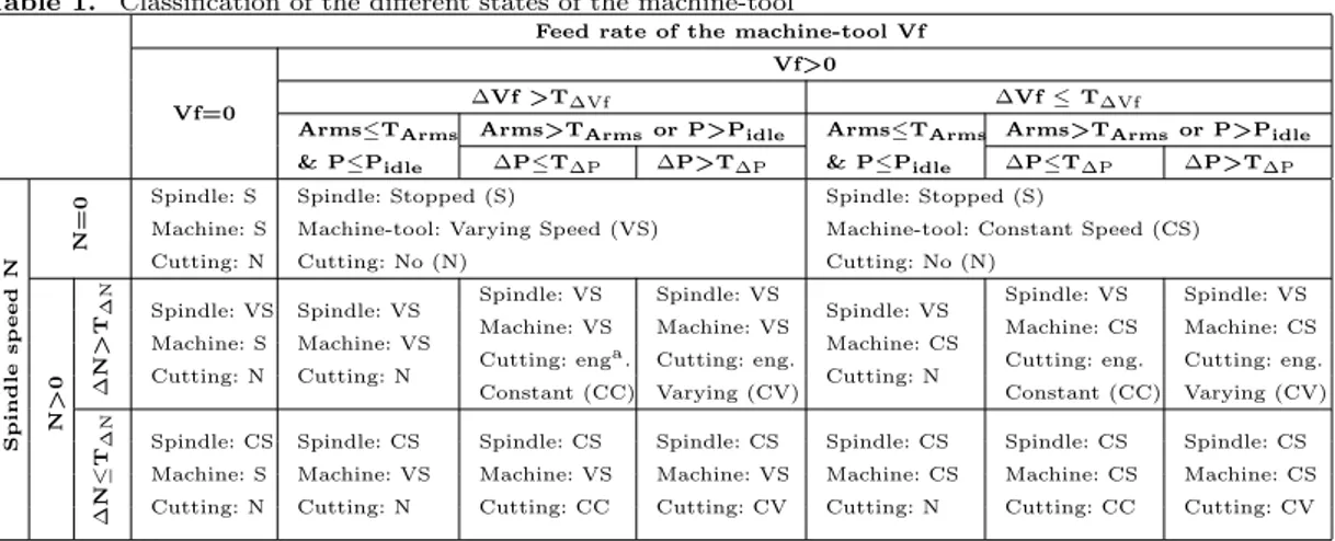
From these three contextual information, 17 potential states for the machine-tool can be defined (cf. Table 1). The objective is to determine the state of the machine-tool at each instant. Indeed, it will enable accurate data selection and analyses dedicated to the considered state.
Table 1. Classification of the different states of the machine-tool
Feed rate of the machine-tool Vf
Vf=0
Vf>0
∆Vf >T∆Vf ∆Vf ≤ T∆Vf
Arms≤TArms
& P≤Pidle
Arms>TArmsor P>Pidle Arms≤TArms
& P≤Pidle
Arms>TArmsor P>Pidle
∆P≤T∆P ∆P>T∆P ∆P≤T∆P ∆P>T∆P Spindle sp eed N N=0 Spindle: S Machine: S Cutting: N Spindle: Stopped (S)
Machine-tool: Varying Speed (VS) Cutting: No (N)
Spindle: Stopped (S)
Machine-tool: Constant Speed (CS) Cutting: No (N) N > 0 ∆N > T ∆N Spindle: VS Machine: S Cutting: N Spindle: VS Machine: VS Cutting: N Spindle: VS Machine: VS Cutting: enga. Constant (CC) Spindle: VS Machine: VS Cutting: eng. Varying (CV) Spindle: VS Machine: CS Cutting: N Spindle: VS Machine: CS Cutting: eng. Constant (CC) Spindle: VS Machine: CS Cutting: eng. Varying (CV) ∆ N ≤ T ∆N Spindle: CS Machine: S Cutting: N Spindle: CS Machine: VS Cutting: N Spindle: CS Machine: VS Cutting: CC Spindle: CS Machine: VS Cutting: CV Spindle: CS Machine: CS Cutting: N Spindle: CS Machine: CS Cutting: CC Spindle: CS Machine: CS Cutting: CV
aTool cutting with constant tool engagement
These classifications will be performed focusing on a variable X (e.g., feed rate V f , spindle speed N or spindle power P ) and also on the variation of X, noted ∆X (e.g., ∆V f or ∆N ), which is defined by the simple derivative:
∆X = Xn− Xn−1
∆t (1)
where, Xn is the nth measure; Xn−1 is the measure at the previous instant and ∆t is
the data recording period (0.1s). The objective is to calculate a classification threshold T∆X by unsupervised machine learning methods. A previous study (Wang et al. 2019)
compared the performance of GMM with the k-means method; GMM performs better in this context of research work. The classifications are then carried out based on the following rules:
- There are three clusters for machine-tool movements: stopped (V f = 0), moving at constant speed (V f > 0 and ∆V f ≤ T∆V f), or varying speed (V f > 0 and
∆V f > T∆V f);
con-stant speed (N > 0 and ∆N ≤ T∆N); or varying speed (N > 0 and ∆N > T∆N).
In order to know if the tool is cutting materials or not, a classification according to the criteria Arms (root mean square-RMS of vibration acceleration value, in m/s2)
and the spindle power P (kW) is proposed, when the machine is moving (feedrate V f > 0). In machining, it is known that if the tool is cutting, its vibration (Arms) is greater than if the tool is not cutting. It is also known that when the tool is not cutting, the power (P ) will exceed the spindle power corresponding to idle rotation (Pidle). However, there is a subclass called spindle startup where the Arms is also
greater due to the lubrication spindle startup. This subclass should be identified and assigned to the cluster tool not cutting. The proposed business rules are:
- if (P > Pidleor Arms > TArms) and V f > 0, except the subclass spindle startup,
the tool is cutting material;
- if P ≤ Pidle and Arms ≤ TArms, including the subclass spindle startup, the tool
is not cutting material.
The following procedure aims to check if the GMM classifications are correct or not: - Modeling : The contextual classification thresholds are determined, using GMM on different descriptors (∆N , ∆V f , Arms, P and ∆P ). Each machine-tool has different characteristics, so it is necessary to perform an initial training for each machine-tool. One-day data of a machining database is used for this purpose. - Classifying: The classifications are carried out using GMM threshold and the
business rules.
- Validation: The quality of classifications is assessed by confusion matrix, using a vector labeled with actual classes of machine-tool states.
3. Gaussian Mixture Model
The Gaussian Mixture Model is a statistical model used to parametrically estimate the distribution of random variables by modeling them as a mixture of Gaussian distributions. It has been used in several areas such as audio recognition, measurement error modeling (Huang et al. 2005). The principle of GMM is to find an approximation of the probability density f from a sample of n observations of the random vector X = {x1, x2, x3...xn} (where each observation xi is assumed independent) using a
linear combination of several Gaussian components.
To evaluate the quality of the model parameter θ, the probability density associated with the observed data is calculated (Maugis, Celeux, and Martin-Magniette 2009):
f (X, θ) =
k
X
j=1
ajNj(xi|µj, σj) (2)
where, k is the number of Gaussian; aj is the weight of the jthGaussian. It verifies the
probability conditions such as Pk
j=1aj = 1, and 0 ≤ aj ≤ 1; Nj(xi|µj, σj) expresses
the probability that a measure xi is associated with the jth Gaussian. In this context,
the parameters of the model are collectively represented as θ = {aj, µj, σj}.
In the literature, there are several methods for estimating these GMM parame-ters. In the present paper, the Maximum Likelihood method is used to determine the parameters θ.
The main idea of Maximum Likelihood Estimation (MLE) is to find a set of pa-rameter estimates, so that the likelihood of the sample used is maximized. Since the n observations are independent, the likelihood function L(X|θ) can be written as (Bishop 2006): L(X|θ) = f (x1, θ) × f (x2, θ) × · · · × f (xn, θ) = n Y i=1 f (xi, θ) (3)
Then substitute Eq. (2) into Eq. (3) leads to:
L(X|θ) = n Y i=1 k X j=1 ajNj(xi|µj, σj) (4)
It is easier to maximize likelihood than the likelihood function itself. The log-likelihood function is written as:
ln L(X|θ) = n X i=1 ln ( k X j=1 ajNj(xi|µj, σj)) (5)
The problem of estimation by the maximum likelihood method is therefore to find the roots of the following equation:
∂ ln L(X|θ)
∂θ = 0 (6)
In general, maximizing the likelihood function does not have an analytical solution. It is then necessary to use iterative methods. The most common is to use the EM algorithm (Expectation-Maximization) (Feng, Lai, and Kar 2016). However, the EM algorithm needs initial parameters; the most important of them is the number of classes k.
In general, the larger the number of parameters to be estimated into the model, the better the model approaches to the data. However, the complexity of the computation will also increase when there are too many parameters to be estimated. Therefore, a compromise must be found; this is the goal of the the Bayesian Information Criterion (BIC). The BIC is defined as follow (Schwarz et al. 1978):
BIC(k) = 2 × M ax(ln(L(X|θ))) − Nmln(n) (7)
where, M ax(ln(L(X|θ)))is the maximized log-likelihood function, Nm is the number
of parameters to be estimated in this model (3 per Gaussian: weight, mean and standard deviation), n is the number of observations, and k is the number of classes.In the BIC, the term (Nm) penalizes the complexity of the model. Therefore, BIC is
maximized for most parsimonious setting, i.e., with small Nm, and larger likelihood.
4. Validation of the Gaussian model by silhouette method
In this section, the previously proposed machine learning procedure by GMM is applied to database from four different machine-tools in two factories producing aeronautical structural parts:
- The machine-tool #1 is a Forest Aeromill for aluminum machining, in company #A;
- The machine-tool #2 is a Forest Aerostar for aluminum machining, in company #A;
- The machine-tool #3 is a Mazak Mazatrol for aluminum machining, in company #B;
- The machine-tool #4 is a Mazak i800T for titanium machining, in company #B. An Emmatools device was installed on each machine-tool, and the machining data were collected for months during industrial productions. The classifications should determine:
- If the spindle is rotating (at constant or varying speed) or not, according to the classification on the descriptor ∆N ;
- If the machine-tool is moving (at constant or varying speed) or not, according to the classification on the descriptor ∆V f ;
- If the tool is removing materials (with constant or varying tool engagement) or not, according to the classification descriptor of Arms, P and ∆P .
For each machine-tool, the determination of the number of context classes is crucial and required for the Gaussian model that follows (in order to identify the classification thresholds for the business rules). The proposed method is:
- Apply GMM for each descriptor (∆N , ∆V f , Arms, P and ∆P ) for different numbers of classes (1, 2,..., k). For each number of classes, a BIC value can be determined according to Eq. (7), in order to evaluate the model.
- Compute the BIC in relation to the number of classes for each descriptor. In the present case, each BIC value converges to a maximum.
- Chose the minimal number of context classes required
In this paper, a class number based on 90% of the BIC maximum is chosen. In this way, the class number is reduced and enables better interpretability of the results.
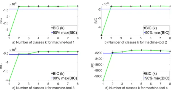
4.1. Silhouette method on the variation of spindle speed
The Gaussian model analyzed by BIC on the variation of spindle speed ∆N is done on the four machine-tools. Fig. 2 shows the results: the BIC value reaches 90% of the BIC maximum with 2 classes. Thus, ∆N was classified into 2 classes, 2 clusters that correspond to the constant and varying spindle rotation. The experimental data confirm what was assumed in Table 1.
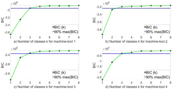
4.2. Silhouette method on the variation of axis speed
The Gaussian model analyzed by BIC on the variation on ∆V f are performed on four machine-tools as shown in Fig. 3. The figure shows that the BIC value reaches 90% of the BIC maximum with 2 classes. Thus, ∆V f was classified into 2 classes, 2 clusters
Figure 2. BIC on ∆N issued from the 4 machine-tools
that correspond to constant and varying motion of the machine-tool.
Figure 3. BIC on ∆V f issued from the 4 machine-tools
4.3. Silhouette method on vibrations and power
The descriptors Arms (vibration) and P (spindle power) are used to determine if the tool is removing materials or not (cf. 1). To determine the number of classes required, Gaussian model analyses by BIC on Arms as shown in Fig. 4 and P Fig. 5. 4 different machine-tools are used in order to validate the results.
The figure shows that the BIC value reaches 90% of the BIC maximum with 3 classes. Thus, k=3 and the vibrations Arms and the power P were classified into 3 classes. The 3 classes are interpreted as: not cut, low material removal and high material removal.
Figure 4. BIC on Arms (when N constant et Vf>0) issued from the 4 machine-tools
Figure 5. BIC on P (when N constant et Vf>0) issued from the 4 machine-tools
5. Contextual classification of the material removal
Once the class number determined by BIC, the classification thresholds are identified from one-day data by GMM. Then, the business rules are applied, leading to the classification. This section presents the classification. GMM is applied to the collected data in the context of spindle rotation at constant speed and axis motion (V f > 0) see Table 1. Two datasets illustrate the approach: machine-tools #2 and #3 for aluminum machining.
5.1. Modeling and classification for machine-tool #3
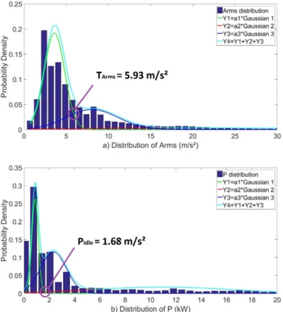
The distribution of Arms in this class (N constant and V f > 0) is modeled by 3 Gaussians (see section 4).
- a Gaussian represents the class tool not cutting (Y1 green), - another the class tool cutting (Y3 blue),
- the 3rd Gaussian represents ’severe machining vibrations’ (Y2 red).
Figure 6. Distribution of Arms and P (when N constant and Vf>0) modeled by GMM for machine-tool #3
The distribution of Y4 (in cyan) is the sum of these 3 Gaussians (Y4=Y1+Y2+Y3) as shown in Fig. 6(a). The threshold TArms is defined as the intersection between the
Gaussians Y1 and Y3, in order to minimize classification errors (false positives and negatives). The threshold is identified: TArms =5.93 m/s2 is obtained.
Applying the same method, P is modeled by 3 Gaussians: - one Gaussian represents the class tool not cutting (Y1 green),
- another represents the class tool cutting with low material removal (Y3 blue), - the 3rd Gaussian (Y2 red) models the class tool cutting with high material
re-moval.
The distribution of Y4 (cyan) is the sum of these 3 Gaussians (Y4=Y1+Y2+Y3), as shown in Fig. 6(b). The threshold is chosen at the intersection between the Gaussian tool is not cutting and the other Gaussian tool cutting with high material removal, thus obtaining Pidle =1.68 kW.
A combination of the two sensors measurements is performed. Thus, for data where spindle is rotating at constant speed and axes are moving (V f > 0) see Table 1, if Arms > TArms or P > Pidle, the data is assigned to the class tool cutting.
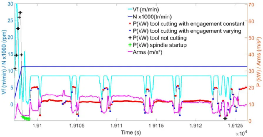
Fig. 7 presents data from machine-tool #3 as well as the result of the classification. The tool not cutting class is represented by black ”+” signs on the P power curve,
the tool cutting class is presented by red and blue dots. The tool cutting class can be classified into two sub-classes: tool cutting with constant engagement (in red points) and tool cutting with varying engagement (in blue points) by classification on ∆P (see Table 1). When the spindle has reached its target speed (N =11250 rpm in Fig. 7), the tool does not cut immediately. There is a subclass called spindle startup. This class is represented by green ”+”. It is defined by the following rule: from the reach of the target speed N until the power exceeds the no-load power Pidle (which represents the
beginning of machining). Identify this state permits to eliminate parasitic vibrations related to lubrication spindle startup, which would otherwise lead to classification errors. The subclass spindle startup is also assigned to the cluster tool not cutting.
Cyan line represents V f , blue line N , pink line Arms. The tool engagement is correctly detected.
Figure 7. Classifications of material removal for machine-tool #3
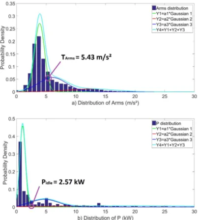
5.2. Modeling and classification for machine-tool #2 The Arms distribution is modeled by 3 Gaussians (see section 4):
- a Gaussian represents the class tool not cutting (Y1 green), - another the class tool cutting (Y3 blue),
- the 3rd Gaussian represents ’severe machining vibrations’ (Y2 red).
The distribution of Y4 (in cyan) is the sum of these 3 Gaussians (Y4=Y1+Y2+Y3) as shown in Fig. 8(a). The threshold TArms is defined as the intersection between the
Gaussians Y1 and Y3, in order to minimize classification errors (false positives and negatives). This enables to identify TArms =5.43 m/s2 for the machine-tool #2.
Applying the same method, P is modeled by 3 Gaussians: - one Gaussian represents the class tool not cutting (Y1 green),
- another represents the class tool cutting with low material removal (Y3 blue), - the 3rd Gaussian (Y2 red) models the class tool cutting with high material
re-moval.
The distribution of Y4 (cyan) is the sum of these 3 Gaussians (Y4=Y1+Y2+Y3), as shown in Fig. 8(b). The threshold is chosen at the intersection between the Gaussian tool is not cutting and the other Gaussian tool cutting with high material removal. This leads to Pidle =2.57 kW.
Figure 8. Distribution of Arms and P (when N constant and Vf>0) modeled by GMM for machine-tool #2
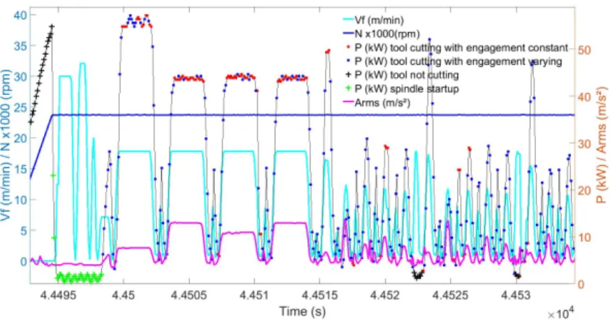
In summary, three classes of the tool engagement are defined.
- tool cutting when Arms > TArmsor P > Pidle; it consists of two subclasses : tool
cutting with constant engagement and tool cutting with varying engagement ; - the tool not cutting when Arms ≤ TArmsand P ≤ Pidleby including the subclass
spindle startup.
Fig. 9 plots the N (rpm), V f (m/min), Arms (m/s2) and P (kW) as well as the classification results in classes (dots and + sign) for machine-tool #2. The material removal is well classified.
6. Method validation
The estimation of the quality of the classification by machine learning isessential to choose an optimal descriptor or combining descriptors for a given data set (Wolpert 1992). Two criteria constitute the quality: accuracy and sensitivity.
6.1. Accuracy
To estimate the accuracy of the classification by GMM, manual data mining was used. In our approach, the classifications based on GMM model conduct to the predicted classes (tool cutting or tool not cutting). The actual classes correspond to 100% true classes that were constituted by manual data mining. The main steps are as follows:
Figure 9. Classifications of material removal for machine-tool #2
- Apply GMM for training on a one-day data and identify the thresholds of TArms
and Pidle. ;
- Choose a data period and use the two thresholds to the set to predict classes: tool cutting and tool not cutting ;
- Go through manual data mining, one point by one point, to obtain the actual classes;
- Compare the predicted with the actual classes and calculate the confusion ma-trix.
Table 2 reports the confusion matrix for 4 hours on the machine-tool #3 and Table 3 the confusion matrix for the machine-tool #2 .
Table 2. Confusion matrix for 4 hours data from the machine-tool #3 Confusion Matrix Tool CuttingActual ClassesTool Not Cutting Predicted Classes Tool Cutting TP=51 476 FP=18
Tool Not Cutting FN=67 TN=92 470
Table 3. Confusion matrix for 4 hours data from the machine-tool #2 Confusion Matrix Actual Classes
Tool Cutting Tool Not Cutting Predicted Classes Tool Cutting TP=60 626 FP=292
Tool Not Cutting FN=938 TN=93 707
Accuracy of the Classification (ACC) is the ratio of correct predictions and is com-puted as follows: ACC = T P +T N +F P +F NT P +T N
The accuracy is obtained for the machine-tool #3: ACC #3 (4h)=99.94%, as well as for the machine-tool #2 is: ACC #2 (4h)=99.21%. The classifications obtained using GMM method are very accurate.
6.2. Sensitivity of the method
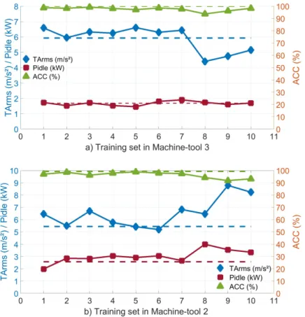
In order to test whether the method is sensitive to the training data set , the cross-validation method can be used. Kohavi et al. (1995) present different cross-cross-validation methods like ’Holdout’, ’Leave-one-out’, ’k-fold’ and ’Stratification’. In this paper, the cross-validation method ’k-fold’ is used. The original sample is divided into k
samples, then one of the k samples is selected as the training set and the (k − 1) other samples will constitute the validation set. The performance score is calculated. The operation is repeated k times so that each sub-sample is used once as a training set. The average of the performance scores is finally calculated to estimate the accuracy of the classifications. Here 10 days were chosen (k=10) as the original sample. The main steps are as follow. For each day:
- Apply GMM to the training set to obtain its thresholds of Arms and P , - Apply these new thresholds to the validation set (nine other days) to obtain the
predicted classes,
- Compare these predicted classes with the actual classes and calculate the con-fusion matrix. The accuracy for each days is obtained.
The thresholds of Arms and P for each day in the training sets as well as correspond-ing accuracy when applycorrespond-ing these thresholds to the validation set for the machine-tool # 3 and the machine-tool # 2 are respectively reported in Fig. 10( a and b). The horizontal dotted lines are the thresholds of Arms and P as well as the corresponding accuracy obtained in the validation set in these two machine-tools.
Figure 10. The new thresholds of Arms and P obtained in the training sets as well as these thresholds obtained in validation sets for (a) machine-tool #3 and (b) machine-tool #2
With 10 sets, the mean accuracy of the classification for the machine-tool #3: ACC(k-fold) #3 (4h)=97.60%, and for the machine-tool #2: ACC(k-fold) #2 (4h)=96.28%. This shows the robustness of the proposed method. The mean accuracy is lower than the one using the same set for training and validation. It is because the thresholds for materials removal or not (TArmsand Pidle) may slightly change as time
goes by, due to the variation of the machine condition (e.g. wear of the spindle). Nevertheless, the mean accuracy obtained is high enough that the thresholds learned by GMM during one-day can be used for any other day of production on the same machine-tool.
7. Application of the contextual classifications for KPIs evaluation on production data
According to the previous validation steps, the contextual classification made by the proposed method is accurate and robust. Thus, Key Performance Indicators can be calculated based on this contextual classification. For example, it is interesting for the industry to know:
- Smart Overall Equipment Effectiveness (OEE) of the machine-tool.
Fig. 11 stresses the real machine-tool use rate during the complete spindle lifetime (215 days) for machine-tool # 2. The contextual classification enables to determine at each instant if the machine-tool is stopped (in red), removing material (cyan and yellow) or not (in pink). Then, during machining, operations dedicated to high material removal (in cyan) or low material removal (i.e. finishing operations, in yellow) can be aggregated separately (contrary to classical OEE computations). Note that the factory where data were collected works in a three-shift system 5 days a week, and that stopped times of Fig. 11 include week-end.
Figure 11. Machine-tool OEE during the complete spindle lifetime for the machine-tool # 2
- The programs which generate more chatter when cutting materials. - The tools which induce more chatter when cutting materials.
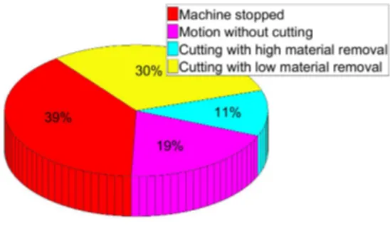
For the denoising reasons, the criterion for chatter detection Godreau et al. (2019) should be evaluated only in the context where the tool is cutting. The proposed clas-sification method is therefore applied. Fig. 12(a) shows the pie chats representing the faulty work-piece programs in terms of chatter for the complete spindle lifetime of machine-tool # 2. Fig. 12(b) shows the pie chats representing the chatter occurrences ratio per tool for the complete spindle lifetime of machine-tool # 2, which is also evaluated in the context where the tool is cutting.
Figure 12. Pie charts representing the chatter occurrences per workpiece program (a) and per tool (b) during the complete spindle lifetime for machine-tool # 2
8. Conclusion
This paper proposes an original contextual classification of data for smart machining based on unsupervised machine learning by Gaussian mixture model. The following generic contributions were obtained:
(1) Complete business rules for contextual classification,
(2) A methodology, based on GMM and BIC, to determine the different states of the machine-tool,
Those proposition were validated on the raw data used in this paper was collected and stored by the device Emmatools which is installed on four machine-tools in two factories producing aeronautical structural parts.
- A classification of the tool cutting or not, by combining GMM thresholds of vibration measurements Arms and power measurements P , was validated on 2 different machine-tools.
- k-fold validation enables to conclude that the thresholds learned by GMM during one-day can be applied to any other days for the same machine-tool. It was also found that the thresholds learned by GMM during one-day data may slightly change due to the variation of the machine condition.
- this contextual classification permit to obatined precisel KPIs that facilitate decision making.
The learned values of thresholds given in this paper are specific to a given machine-tool, but the proposed machine learning methodology is replicable to any machine-tool.
Acknowledgment
The authors acknowledge the financial support of the French National Research Agency on the ANR SmartEmma project (ANR-16-CE10-0005). They would also like to thank the contributions made by the industrial partners.
References
Bhinge, Raunak, Nishant Biswas, David Dornfeld, Jinkyoo Park, Kincho H Law, Moneer Helu, and Sudarsan Rachuri. 2014. “An intelligent machine monitoring system for energy predic-tion using a Gaussian Process regression.” In 2014 IEEE Internapredic-tional Conference on Big Data (Big Data), 978–986. IEEE.
Bishop, Christopher M. 2006. Pattern recognition and machine learning. springer.
De Castelbajac, Cˆome, Mathieu Ritou, S Laporte, and Benoˆıt Furet. 2014. “Monitoring of distributed defects on HSM spindle bearings.” Applied Acoustics 77: 159–168.
El-Mounayri, Hazim, and Haiyan Deng. 2010. “A generic and innovative approach for inte-grated simulation and optimisation of end milling using solid modelling and neural network.” International Journal of Computer Integrated Manufacturing 23 (1): 40–60.
Feng, Guodong, Chunyan Lai, and Narayan C Kar. 2016. “Expectation-maximization particle-filter-and Kalman-filter-based permanent magnet temperature estimation for PMSM con-dition monitoring using high-frequency signal injection.” IEEE Transactions on Industrial Informatics 13 (3): 1261–1270.
Godreau, Victor, Mathieu Ritou, Etienne Chov´e, Benoit Furet, and Didier Dumur. 2019. “Con-tinuous improvement of HSM process by data mining.” Journal of Intelligent Manufacturing 30 (7): 2781–2788.
Huang, Yonghong, Kevin B Englehart, Bernard Hudgins, and Adrian DC Chan. 2005. “A Gaussian mixture model based classification scheme for myoelectric control of powered upper limb prostheses.” IEEE Transactions on Biomedical Engineering 52 (11): 1801–1811. Kim, Dong-Hyeon, Thomas JY Kim, Xinlin Wang, Mincheol Kim, Ying-Jun Quan, Jin Woo
Oh, Soo-Hong Min, et al. 2018. “Smart machining process using machine learning: A review and perspective on machining industry.” International Journal of Precision Engineering and Manufacturing-Green Technology 5 (4): 555–568.
Kohavi, Ron, et al. 1995. “A study of cross-validation and bootstrap for accuracy estimation and model selection.” In Ijcai, Vol. 2, 1137–1145. Montreal, Canada.
Lenz, Juergen, Thorsten Wuest, and Engelbert Westk¨amper. 2018. “Holistic approach to ma-chine tool data analytics.” Journal of manufacturing systems 48: 180–191.
Liu, Chao, Hrishikesh Vengayil, Ray Y Zhong, and Xun Xu. 2018. “A systematic development method for cyber-physical machine tools.” Journal of manufacturing systems 48: 13–24. Maleki, Elaheh, Farouk Belkadi, Mathieu Ritou, and Alain Bernard. 2017. “A tailored ontology
supporting sensor implementation for the maintenance of industrial machines.” Sensors 17 (9): 2063.
Maugis, Cathy, Gilles Celeux, and Marie-Laure Martin-Magniette. 2009. “Variable selection for clustering with Gaussian mixture models.” Biometrics 65 (3): 701–709.
Morgan, Jeff, and Garret E ODonnell. 2018. “Cyber physical process monitoring systems.” Journal of Intelligent Manufacturing 29 (6): 1317–1328.
Quintana, Guillem, and Joaquim Ciurana. 2011. “Chatter in machining processes: A review.” International Journal of Machine Tools and Manufacture 51 (5): 363–376.
Ritou, Mathieu, Farouk Belkadi, Zakaria Yahouni, Catherine Da Cunha, Florent Laroche, and Benoit Furet. 2019. “Knowledge-based multi-level aggregation for decision aid in the machining industry.” CIRP Annals 68: 475–478.
Rodr´ıguez, Juan J, Guillem Quintana, Andres Bustillo, and Joaquim Ciurana. 2017. “A decision-making tool based on decision trees for roughness prediction in face milling.” In-ternational Journal of Computer Integrated Manufacturing 30 (9): 943–957.
Schwarz, Gideon, et al. 1978. “Estimating the dimension of a model.” The annals of statistics 6 (2): 461–464.
Teti, Roberto, Krzysztof Jemielniak, Garret O’Donnell, and David Dornfeld. 2010. “Advanced monitoring of machining operations.” CIRP annals 59 (2): 717–739.
Wang, Zhiqiang, Catherine Da Cunha, Mathieu Ritou, and Benoˆıt Furet. 2019. “Comparison of K-means and GMM methods for contextual clustering in HSM.” Procedia Manufacturing 28: 154–159.
Wolpert, David H. 1992. “Stacked generalization.” Neural networks 5 (2): 241–259.
Zhang, Chen, and Haiyan Zhang. 2016. “Modelling and prediction of tool wear using LS-SVM in milling operation.” International Journal of Computer Integrated Manufacturing 29 (1): 76–91.
Zhou, Yuqing, and Wei Xue. 2018. “Review of tool condition monitoring methods in milling processes.” The International Journal of Advanced Manufacturing Technology 1–15.