HAL Id: hal-01879016
https://hal.archives-ouvertes.fr/hal-01879016
Submitted on 26 Feb 2019
HAL is a multi-disciplinary open access archive for the deposit and dissemination of sci-entific research documents, whether they are pub-lished or not. The documents may come from teaching and research institutions in France or abroad, or from public or private research centers.
L’archive ouverte pluridisciplinaire HAL, est destinée au dépôt et à la diffusion de documents scientifiques de niveau recherche, publiés ou non, émanant des établissements d’enseignement et de recherche français ou étrangers, des laboratoires publics ou privés.
Molecular tagging velocimetry by direct
phosphorescence in gas microflows: Correction of Taylor
dispersion
Hacene Si Hadj Mohand, Aldo Frezzotti, Juergen Brandner, Christine Barrot,
Stéphane Colin
To cite this version:
Hacene Si Hadj Mohand, Aldo Frezzotti, Juergen Brandner, Christine Barrot, Stéphane Colin. Molecular tagging velocimetry by direct phosphorescence in gas microflows: Correction of Tay-lor dispersion. Experimental Thermal and Fluid Science, Elsevier, 2017, 83, pp.177 - 190. �10.1016/j.expthermflusci.2017.01.002�. �hal-01879016�
1
Molecular tagging velocimetry by direct
phosphorescence in gas microflows: correction of
Taylor dispersion
Hacene SI HADJ MOHAND, Aldo FREZZOTTI, Juergen J. BRANDNER, Christine BARROT, Stéphane COLIN
H. Si Hadj Mohand, C. Barrot and S. Colin ()
Institut Clément Ader (ICA), Université de Toulouse, CNRS – INSA – ISAE – Mines Albi – UPS, Toulouse, France.
e-mail: stephane.colin@insa-toulouse.fr
A. Frezzotti
Dipartimento di Scienze & Tecnologie Aerospaziali, Politecnico di Milano, Campus Bovisa Sud,via La Masa 34,20156 Milano, Italy
J. J. Brandner
Karlsruhe Institute of Technology, Institute for Micro Process Engineering, Campus Nord, Hermann-von-Helmholtz-Platz 1, 76344 Eggenstein-Leopoldshafen, Germany
Abstract: Molecular tagging velocimetry is a little-intrusive technique based on the properties
of specific molecules able to emit luminescence once properly excited. Several variants of this technique have been successfully developed for analyzing external gas flows or internal gas flows in large systems. There is, however, very few experimental data on molecular tagging velocimetry for gas flows in mini or microsystems, and these data are strongly affected by the molecular diffusion of the tracer molecules. In the present paper, it is demonstrated that the velocity field in gas microflows cannot be directly deduced from the measured displacement field without taking into account Taylor dispersion effects. For that purpose, the benchmark case of a Poiseuille gas flow through a rectangular channel 960 µm in depth is experimentally investigated by micro molecular tagging velocimetry using acetone vapor as a molecular tracer. An appropriate reconstruction method based on the advection diffusion equation is used to process the data and to correctly extract the velocity profiles. The comparison of measured velocities with flowrate data and with theoretical velocity profiles shows a good agreement, whereas when the reconstruction method is not implemented, the extracted velocity field exhibits qualitative and quantitative anomalies, such as a non-physical slip at the walls. The robustness of the reconstruction method is demonstrated on flows with light and heavy molecular species, namely helium and argon, at atmospheric as well as at
2
lower pressure conditions, for which diffusion effects are stronger. The obtained results represent an encouraging step for future analysis of rarefied gas microflows.
Keywords: Molecular tagging velocimetry · MTV · confined gas flows · molecular diffusion · Taylor dispersion
1 Introduction
The last two decades have witnessed a rapid development of micro-electromechanical systems (MEMS) leading to the emergence of a number of new microfluidic applications involving gas microflows in various technical fields. Gas microflows are notably involved in micro heat exchangers [1] designed for chemical applications or for cooling electronic components, in fluidic micro-actuators developed for active flow control purposes [2], in micronozzles used for the micropropulsion of nano and picosats [3], in micro gas chromatographs [4], gas analyzers [5] or gas separators [6], in vacuum generators and in Knudsen micropumps [7] as well as in some microfluidic-based in vitro devices such as artificial lungs [8]. Similar flows are also observed in porous media with applications relative to the extraction of shale gas [9]. In most of these microsystems, gas flows evolve in the slip flow regime with a Knudsen number, which is the ratio of the molecules mean free path over a characteristic length of the microsystem, in the range [10-3; 10-1]. This slightly rarefied regime is characterized by rarefaction effects located at the walls, where a velocity slip and a temperature jump take place [10]. Models in this so-called slip flow regime can be simply based on the usual Navier-Stokes-Fourier equations associated with specific boundary conditions, various forms of which have been proposed in the literature. They require the knowledge of accommodation coefficients which depend on the gas species and on the wall material and roughness [11] as well as on the temperature [12]; these models lead to more or less complex solutions for heat transfer [13] and fluid flow [14] but there is no scientific consensus about the best way to determine the values of these coefficients. Experimental data are then necessary to improve the open discussion about the accuracy and limits of applicability of the various slip boundary models proposed by different authors. Experimental techniques described in the literature, however, mainly concern measurement of global data [15]. Most of the publications provide flowrate data through microchannels as a function of the pressure drop and the Knudsen number [16-24]. This global information is not sufficient to separately analyze the role of the
3
velocity slip model and the role of the a priori unknown accommodation coefficients. Unfortunately, there are few available data on local fields and most of them are pressure field data obtained by pressure-sensitive molecular films (PSMF) [25, 26]. Up to now, there are no experimental data in the literature on velocity fields in rarefied gas microflows. It is then crucial to develop accurate velocimetry techniques adapted to the specific features of gas microflows. Among these techniques, the most usual one is the micro particle image velocimetry (µPIV) technique. It is widely and successfully used for liquid microflows, but the main limitation of its application for analyzing gas flows at microscale is linked to the Brownian motion of the small tracer particles [27], which limits the accuracy of the cross-correlation process required to recognize particle patterns and extract velocity fields. As a consequence, µPIV experiments in gases have been up to now limited to very few studies in millimetric channels and in non-rarefied regimes [28, 29].
On the other hand, micro molecular tagging velocimetry (µMTV) could be a well-suited technique able to avoid this difficulty since it is not based on a particle pattern identification. µMTV relies on the properties of tracer molecules which can experience short or relatively long lifetime luminescence once excited with a light at an appropriate wavelength.
All MTV techniques are based on the chemistry of molecules in electronic excited states and can be classified according to their basic mechanisms. A detailed description of the four basic mechanisms involved in MTV techniques can be found in [30]. As explained below, only some of them are suitable for gas-phase flow analysis, under certain conditions.
- The first mechanism is MTV by absorbance. The associated techniques are generally called laser induced photochemical anemometry (LIPA) or laser photochemical velocimetry (LPV), and their principle is based on an image produced by a photochromic dye and relies on measuring absorbance [31]. The use of MTV by absorbance is limited to liquid flows.
- The second mechanism is MTV by vibrational excited state fluorescence. It has led to the Raman excitation plus laser-induced electronic fluorescence (RELIEF) technique initially developed by the group of Miles [32-37] for molecular tagging in unseeded air flows. The technique is sophisticated but challenging to implement, because it requires three photon sources with different frequencies, two to tag and one to interrogate. In addition, its use is limited to oxygenated flows, as the molecular tracer is oxygen brought to a vibrational excited state.
4
- The third mechanism is MTV by photoproduct fluorescence. This mechanism is used in the photo-activated nonintrusive tracking of molecular motion (PHANTOMM) technique initially introduced by Lempert and co-workers [38], and can be considered as the luminescent counterpart to LIPA. It requires two or three laser sources. The initial excitation pulse is used to produce the tracer, which is tracked by detecting emitted light, instead of transmitted light as in the case of LIPA. Although MTV by photoproduct fluorescence was initially developed for liquid flows, gas phase flows can also be imaged by the PHANTOMM technique or its variants, which can involve various tracers such as ozone in the oxygen tagging velocimetry (OTV) technique [39], hydroxyl radicals in the hydroxyl tagging velocimetry (HTV) technique suitable for gases containing water vapor [40], C, C2 and CN molecules produced by the
photolysis of hydrocarbons [41] or nitric oxide generated from nitrous oxide in the N2O MTV technique [42]. The air photolysis and recombination tracking (APART)
technique is also suitable for the investigation of air flows and does not require any seeding [43]. As the common mechanism of these different variants is based on the fluorescence and not on the phosphorescence of a tracer, and due to the intense and short lifetime of fluorescence, the technique is very little sensible to oxygen quenching, which is an advantage. Its implementation, however, requires two or three laser sources, and except in the case of the N2O MTV technique, the relative low
lifetime of the generated tracers has up to now limited its use to high velocity, typically supersonic, gas flows.
- The fourth mechanism, called MTV by direct phosphorescence, is the more straightforward and simplest technique to implement, as it requires only one photon source. MTV by direct phosphorescence is an appropriate technique for analyzing non oxygenated gas flow. The gas is seeded with tracer molecules, such as acetone or diacetyl, able to experience a long lifetime phosphorescence, once excited by a single laser. The long lifetime tracer is then the excited state molecule itself, which displacement can be imagined by monitoring the emanating phosphorescence. After emission of a photon, the molecule comes back to its initial state and is then re-usable for a possible new laser excitation. Typically, a single laser beam is required to tag tracer molecules along a line [44] or on a grid [45]. The molecules luminescence is then detected at two successive times and the analysis of the tagged line displacement or of the grid deformation allows the determination of the velocity field.
5
As MTV is a little-intrusive technique that uses molecular tracers, another advantage compared to PIV is to provide a homogeneous repartition of the tracer within the background gas and to avoid the risk to form any aggregate of particles at the wall. Nevertheless, at microscale, μMTV also presents some challenging issues. First, the spatial resolution of the technique is constrained by the laser beam diameter, with a typical minimum value of the order of 30 μm, which requires operating in channels with a hydraulic diameter at least of the order of 1 mm. For this reason, in order to reach the desired Knudsen number range [10-3 – 10-1], corresponding to the slip flow regime, the pressure has to be reduced. Second, although the Brownian motion is not an issue in itself, the diffusion of the molecular tracer within the main fluid can bias the measurement, and this effect can be increased with the reduction of pressure required to reach rarefied regimes.
Since its first developments in the 80s’, the efficiency of MTV has been widely demonstrated for liquid flows [30] at mini [46, 47] and micro [48, 49] scales. Its application to gaseous flows has been validated in external flow configurations at millimetric scales [40, 50-52] and recently at micrometric scales [53]. Molecular tagging has also been implemented to measure number density distributions in a supersonic flow inside a millimetric convergent-divergent nozzle [54].
On the other hand, the first attempts to measure gas flows velocities by MTV inside devices with millimetric or sub-millimetric dimensions are quite recent and the techniques were based on MTV by direct phosphorescence using acetone as tracer molecule [44, 55, 56] or on MTV by photoproduct fluorescence using nitric oxide as tracer molecule [57]. These few preliminary measurements have been made in rectangular channels using one dimensional molecular tagging velocimetry (1D-MTV); in this case a single line or a series of parallel lines are tagged perpendicularly to the flow direction (Fig. 1).
6
Fig. 1: 1D-MTV principle
The component of the displacement in the direction of the flow can then be obtained. Although 1D-MTV has some limitations compared with 2D-MTV and stereoscopic (3D-) MTV, its advantages are a simpler implementation and a higher spatial resolution in the vicinity of the wall [58]. This makes 1D-MTV a promising technique for capturing velocity slip at the wall in slightly rarefied regimes.
However, in the recent MTV experimental studies of gaseous flows in a millimetric rectangular channel [44, 57], the velocity profile, when it is simply deduced from an homothety of the streamwise displacement profile, appears to be more flatten than the expected theoretical velocity profile and an artificial velocity slip is observed at the wall. Samouda et al. suggested that the effects of spanwise molecular diffusion could explain this behavior [44]. Actually, the tracer molecules appear to become displaced at the wall through advection in the MTV method, even when there is no velocity slip at the wall. The mechanism responsible for the displacement of the tracer at the wall is illustrated in Fig. 2. A tracer molecule close to the wall, where the macroscopic velocity is almost zero, can diffuse away from the wall in a region where the advection is not zero, is then advected in the direction of the flow and can finally diffuse towards the wall, resulting in a displacement parallel to the wall. This molecular slip is observed by MTV but does not correspond to any macroscopic velocity slip at the wall. The effects resulting from the combined action of molecular diffusion
7
and the variation of velocity over the cross-section in a shear flow are known as Taylor dispersion [59].
Fig. 2: Molecular slip at the wall due to the combined effect of advection and transverse diffusion
Similar conclusions have also been recently drawn for liquid microflows by Schembri et al. who used photobleached molecular tracers for velocimetry purpose [60]. Although diffusion is much less significant in liquids, the authors showed that the velocity close to the walls could be overestimated due to the combination of molecular diffusion and shear stress. They demonstrated that this error, limited to a near wall region of a few micrometers thick, could be controlled by limiting the diffusion of fluorophore molecules or minimizing the bleaching time. Taylor dispersion has also been considered by Garbe et al. in an experimental analysis of liquid flow by µMTV [61]. The authors have proposed a velocity reconstruction method, aimed at correcting the diffusion effects and based on the inversion of the advection-diffusion equation. This method, which is sensitive to the experimental noise, is specific to a Poiseuille flow assuming a parabolic velocity profile.
Regarding Taylor dispersion in gas microflows, a Direct Simulation Monte Carlo (DSMC) study, led by Frezzotti et al., showed that even in the continuum regime, the tagged molecules are subject to significant molecular diffusion [62]. In case of slip flow, the mechanism illustrated in Fig. 2 leads to an enhancement of the molecular slip observed by MTV at the wall. A comparison between the molecular motions simulated by DSMC and calculated by the advection-diffusion equation was detailed and permitted to conclude that the diffusion of tracer molecules caused by their Brownian motion has a significant impact on MTV signals. As a consequence, the velocity field cannot be directly deduced from a homothetic transformation of the measured displacement in the direction of the flow and diffusion effects have to be taken into account during the data processing, especially in the slip flow regime where the diffusion effects become very significant. The authors proposed a velocity reconstruction method, based on the advection-diffusion equation, able to extract the velocity
8
field from a displacement field by taking into account diffusion effects, without reversing the advection-diffusion equation. The method has been validated on numerical data generated by DSMC, but it has not been tested on real experimental data yet.
The present paper details a MTV investigation of gas flows by direct phosphorescence in a 960 µm deep rectangular channel, focusing on molecular diffusion effects and taking them into account with an appropriate data processing based on the above mentioned velocity reconstruction method. The slip flow regime is not directly investigated in this paper, due to a too low luminescent signal obtained at a few hundreds of Pa, which is the required pressure for observing slip at the wall in a 1 mm deep channel. However, even in a regime without velocity slip at the wall, the molecular slip due to diffusion is already significant at sub-atmospheric pressure and must be corrected by the reconstruction method to extract the real velocity profile. This reconstruction method is briefly described in Section 2. The experimental setup is presented in Section 3. MTV data at atmospheric and sub-atmospheric pressures are then processed and compared to theoretical velocity profiles and flowrate measurements in Section 4. Concluding remarks and perspectives are finally proposed in Section 5.
2 Molecular diffusion modeling and velocity reconstruction
method
We consider a laminar and fully developed steady pressure-driven flow in a long rectangular channel (see Fig.1). The channel length, height and width are L Lx, z and Lyrespectively. It is assumed that Lx? Lz ? Ly, which means that entrance effects are negligible and that the flow can be considered as a planar flow between parallel plates, near the central xy plane (see Fig.
7, below). When the pressure difference is small compared to the mean pressure, the mean displacement s y t of the initially tagged molecules is given by the advection-diffusion x( , ) equation [62] 2/1,2 ² ( ) ² x x x s s u y D t y , (1)
9
( ,0) 0
x
s y (2)
and the boundary conditions
0 at / 2 x y s y L y , (3)
where u y is the velocity profile and x( ) D2/1,2 is the diffusion coefficient of the tracer molecules (index 2) in the mixture containing both tracer and background gas molecules (index 1). Its value is deduced from the Chapman-Enskog estimation of diffusivity by considering Lennard-Jones intermolecular interactions [63]. The diffusion coefficient D2/1,2 is
thus computed from the binary tracer-background gas diffusion coefficient D and the tracer 2/1
self-diffusion coefficient D , following Blanc’s law [64] 2/2
1 1 2 2/1,2 2/1 2/2 D D D , (4)
where 1 and 2 are the background and tracer gas molar fractions, respectively.
An immediate consequence of Eq. (1) is that the streamwise displacement averaged along the
spanwise y-direction, 2 2 ( ) 1 Ly ( , ) x y Ly x s t L s y t dy
, evolves in time as ( ) x x s t u t, (5)where uxis the mean velocity of the flow. This provides the possibility of a direct calculation of the mean velocity from the time evolution of the average displacement in the x-direction. In addition, when the diffusivity and velocity gradient are small, the last term in Eq. (1) vanishes and the equation results in the simple relation ux sx t sx t which is commonly used in tagging velocimetry [52, 58, 65].
In confined gas flows, however, both diffusivity and velocity gradients are large, and the unknown velocity profile can be extracted from the measured displacement profile by solving Eq. (1). The first step of the reconstruction method consists in approximating the velocity profile u y by a sum of x( ) N basis (typically polynomial) u U y functions, as: k( )
0 ( ) ( ) u N x k k k u y a U y
. (6)Secondly, for each basis velocity U y , a corresponding basis displacement k( ) S y t is k( , ) directly obtained by solving Eq. (1) [66] and recasting the solution in the form
10 /2 /2 ( , ) ( , ', ) ( ') ' y y L k k L S y t G y y t U y dy
(7)where G y y t( , ', ) is the Green function associated to Eq. (1). The expression of the displacement s y t is then given by: x( , )
0 ( , ) ( , ) u N x k k k s y t a S y t
. (8)The unknown superposition coefficients a appearing in the velocity expansion (6) are the k
same appearing in the displacement expression (8). Hence, the unknown velocity field is determined by deducing the values of the coefficients a , from a least square approximation k
of the experimental displacement profile exp
( , )
x
s y t , i.e. by minimizing the quadratic error
2 exp 0 ( , ) , u N s x k k k E s y t a S y t
.The application of this reconstruction method to DSMC simulations [62] has shown a very accurate velocity reconstruction from displacements, for Knudsen numbers lower than 0.05, i.e. within the continuum and slip flow regimes. The reconstruction becomes less accurate, however, for Knudsen numbers of the order of, or higher than, 0.1, where the displacement rapidly decays to an almost flat shape, easily hidden by the inherent noise of the displacement data.
The above-described reconstruction method is now applied to experimental displacements measured by MTV in the continuum regime.
11
Fig. 3: Schematics of the experimental setup
3.1. MTV setup
The classical 1-D MTV method is used in this study. A schematics of the experimental setup is shown in Fig. 3. The excitation is made by a frequency-quadrupled dual frame Nd: YAG laser with a wavelength of 266 nm. The laser generates 4 ns pulses at a frequency of 10 Hz, and provides a beam with a maximum energy of 30 mJ, reduced to 1 mJ with an integrated attenuator. The initial laser beam has a 6 mm diameter, and it is focused with a diaphragm and a focusing lens down to a diameter d035µm. Consequently, the laser beam initially tags tracer molecules within a thin circular cylinder perpendicular to the flow direction.
The initial and delayed luminescent lines, corresponding to fluorescence and phosphorescence signals, respectively, are collected by a 12-bit progressive scan camera with a CCD detector coupled to a 25 mm intensified relay optics (IRO). The 1376×1040 pixels CCD sensor has an operating frequency of 10 frames per second. The optics of the camera results from the assembly of 105 mm and inverted 28 mm Micro Nikkor lenses. It has been checked with a camera test card that there was not any measurable barrel or pincushion distortion of the images in the region of interest, due to either the optics or the IRO. As a consequence, the images did not require any unwarping before their data processing detailed in section 3.4. In addition, the horizontality and perpendicularity of the channel and optic axis have been checked using rulers, set squares and a spirit level, and they were adjusted by wedges. The parallelism of the CCD and the channel was checked by taking a picture of the camera test card aligned with the channel lateral side. The verticality of the laser beam (i.e. its perpendicularity to the channel axis and to the optical axis) was ensured by using a specially designed set square tool with two pin holes aligned perpendicularly to its horizontal support put on the upper side of the channel. The laser guiding arm was adjusted such that the beam went through the two pin holes. The fluorescent images obtained just after tagging confirmed the good alignment of the beam.
In order to increase the level of the signal, 4×4 binning has been activated leading to an area of 344 × 260 px covering a 5.5 × 4.16 mm2 physical domain, which gives a resolution of 16 µm/px.
12
3.2. Flow circuit
The background gas supplied by the gas bottle flows through a small reservoir placed between valves V1 and V2 to create a capacitance in order to smooth possible pressure fluctuations. The gas mixture composed of the background gas (argon or helium) seeded with tracer gas (acetone) molecules, is generated by bubbling the background gas in a thermally regulated liquid acetone bath. This bath is equipped with a thermocouple and a pressure sensor which allow the determination of the mixture composition, assuming saturation conditions.
The flow cell consists in a rectangular channel placed between inlet and outlet small tanks equipped with pressure capacitive gauges, providing real time pressures p and in p in the out
inlet and outlet reservoirs, respectively. Local pressure losses are due to the restrictions caused by the connection fittings between the tanks and the channel, and consequently the local pressure at the channel ends is not accurately known. At the outlet of the channel, valve V5 connects the circuit to a vacuum pump for measurements at sub-atmospheric pressure, whereas valve V6 gives an access to a balloon with a calibrated volume Vb2L in order to couple MTV measurements with flowrate data when operating at atmospheric pressure, the flowrate through the circuit being measured by timing the draining of the balloon, with a relative standard uncertainty of 1.8 %. More details on the description of this flowrate measurement technique can be found in [18].
3.3. Flow cell
The 960 µm high, 5 mm wide and 200 mm long channel has been machined in a layer of polyetheretherketone (PEEK). This material has been selected among various thermoplastic polymers because of its excellent chemical compatibility, especially to acetone, its good sealing properties and thermal stability [44].
For the laser access, Suprasil® optical windows have been integrated in both upper and lower walls of the channel (at y Ly 2 ), allowing the UV laser beam to cross the flow in the mid-plane (z=0) of the channel cross-section. The optical access for the camera is laterally ensured by Borofloat® glass plates, located on both sides of the channel (at z Lz 2 ). Suprasil® is a special grade of fused silica, selected for its high transparency to UV wavelengths and its limited own luminescence, whereas Borofloat® has been chosen for its mechanical properties and its transparency to the luminescent signal emitted in the visible wavelengths range.
13
A particular attention is paid when operating at sub-atmospheric pressure: due to the difference of pressure inside and outside the channel, the distance between the upper and lower walls of the channel, Ly, can be reduced because the channel structure is not fully rigid.
Following a series of different tests operated at various pressures, the depth of the channel can slightly change. Therefore, the location of the channel walls is systematically optically measured when the pressure conditions are changed or when a new experimental campaign is launched. At atmospheric pressure, the measured depth was Ly 960µm, and for flows at a lower pressure of the order of 50 kPa, the measured depth was Ly 944µm. In every case, the location of each walls is determined with an accuracy of 1 pixel, corresponding to 16 µm after 4×4 binning.
3.4. Data acquisition and processing
The acquisition of the luminescent signal is performed with an on-chip integration method by selecting a CCD exposure time long enough to capture a series of laser pulses. Typically, the CCD is opened during 10 s, allowing to integrate the signal relative to 100 laser shots in a single "cumulative" image. During these 10 s, the IRO is open during a short period
t t; t
after each laser shot (triggered at ti 0) in order to capture and sum on a single image the luminescence signal of the tracer molecules emitted at time t after each laser shot. The gate
t
is short compared to the delay t. 50 cumulative images are then captured and averaged, and consequently each presented profile is a result from 100×50=5000 laser shots. Details on this technique, which dramatically increases the signal to noise ratio, can be found in [44]. As shown in the upper left corner of Fig. 4, a single image, even when it cumulates 100 laser shots, is not directly exploitable for extracting a displacement profile. On the other hand, the raw displacement profile and the molecular diffusion are clearly visible in the upper right corner of Fig. 4, after the averaging of 50 single images similar to the previous one. As shown on the graph which illustrates the extracted value of the displacement on the channel plane of symmetry (y0) as a function of the number of single images used for generating the averaged image, an averaging of at least 30 single images is necessary before processing the data, following the technique illustrated in Fig. 5.
14
Fig.4: Influence of the number of averaged images to extract the displacement profile. Example of displacement measured at the center of the channel (y0) in the case of a flow of argon
with pin42.7 kPa, pout 42.0kPa and T294 Kat tk 130 µs after the laser shots.
The upper left image is a single image cumulating 100 laser shots.
The upper right image in an averaged image obtained from the averaging of 50 single images similar to the left image (it corresponds to a total of 5000 laser shots).
The gate, i.e. the duration of the IRO opening for each single image capture, has been fixed to 1 µs. As the maximum velocity of the investigated flows is 10 m/s, the maximum displacement of the tagged molecules is 10 µm during the exposure. This displacement is lower than the 16 µm pixel size, which allows to avoid any error in the velocity measurement due to the integration of luminescence of the moving tracer across multiple pixels, as discussed in [67]. This gate is also small compare with the phosphorescence lifetime, and consequently, the decay in signal during the exposure is negligible.
The camera is focused on the mid-plane of the channel, at z0, where the laser beam tags the molecules. The initial image containing the fluorescence signal is captured at tti, immediately after the laser pulse generated à t0
0 ti 10ns
and the initial tagged15
vertical straight line xxi is easily determined from the linear fitting of the maximum fluorescence intensity profile extracted at each value of y.
Thereafter, a sequence of k delayed images containing phosphorescence signals are captured at different delays t , typically between 30 and 130 µs after the laser pulse. In order to reduce k
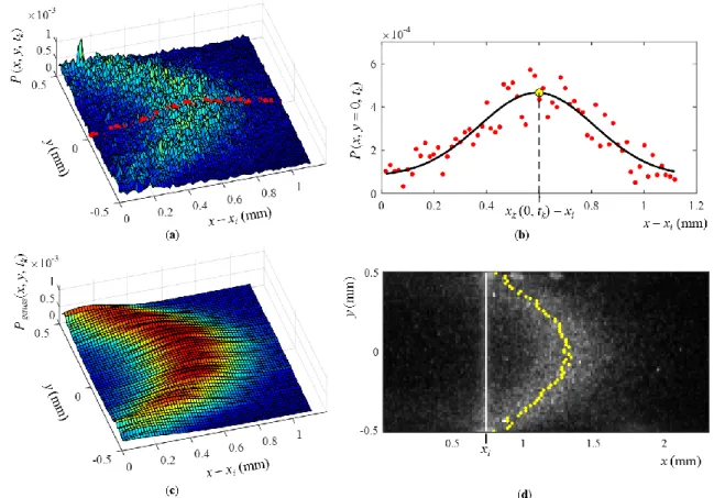
the image noise and remove possible outliers resulting from reflections in the near wall region, an image preprocessing has been systematically performed with Matlab®, using a linear spatial filtering based on correlation, with a 4×4 Gaussian filter [68]. As shown in Fig. 5, the delayed tagged line ( , )x y tk is extracted for each image following a Gaussian fitting of
the phosphorescence intensity [51]: for each y-position, the intensity distribution profile along the x-axis is extracted (Fig. 5-a) and fitted by a Gaussian function Pgauss( , , )x y tk (Fig 5-b) expressed as follow : 2 2 3 ( , ) 2 ( , ) 1 4 ( , , ) ( , ) ( , ) k k x y t y t gauss k k k P x y t y t e y t . (9)
where 1( , )y tk , 2( , )y tk and 3( , )y tk are the parameters of the Gaussian function, and the constant 4( , )y tk is added to take into account the image noise. Finally, the delayed tagged
line is given by (Fig 5-d)
2
( , ) ( , )
k k k
x y t y t (10)
and the resulting displacement profile is obtained by
exp
( , ) ( , )
x k k k i
16
Fig. 5: Example of displacement profile extraction from MTV initial image (ti5 ns)
and delayed image (tk 100 µs). Flow of argon with pin 105.7 kPa, pout 103.7 kPa and T 294 K: (a) Overall distribution P x y( , ) of phosphorescence signal intensity given in arbitrary unit at ttk.
(b) (●) Intensity of the phosphorescence signal in the channel mid-plane y0 at ttk; (▬) Gaussian fitting Pgauss( ,x y0);
(●) Gaussian extremum xk(0, )tk 2(y0, )tk kept for drawing the delayed tagged line displayed in Fig. 5-d. (c) Overall fitted distribution Pgauss( , )x y .
(d) Superposition of the initial and delayed MTV images containing the initial (▬) profile xxi and the delayed (●) extracted profile xxk
y t, k
, providing the displacement profile
exp
,
x k
s y t . The represented region of interest is 144 × 63 px, which corresponds to an area of 2.3 × 1 mm2.
4 Results and discussion
The basis functions used in Eq.(6) for the velocity reconstruction have been chosen with the following polynomial form:
2 ( ) k k y y U y L . (12)
17
For the results presented in this work, a simple decomposition consisting on the two basis function U0 1 and U2( )y
2y Ly
2 has been used. The influence of additional basis functions is discussed at the end of Section 4.1.4.1. Velocity profiles at atmospheric pressure
The first results concern a flow of helium at a mean pressure pmean 102.3 kPa, seeded with acetone with a molar fraction 2 0.22. The experimental raw displacement data obtained at
1 50 µs
t , t2 80 µs and t3 100 µs, following the method described in Section 3.4, are plotted in Fig. 6-a. These data obtained at times t , 1 t and 2 t are represented by diamonds, 3
circles and cross symbols, respectively. The reconstructed method described in Section 2 is then applied and provides reconstructed velocity and displacement profiles. For each case, the reconstructed displacement s y tx( , )k computed from Eq. (8) is plotted in Fig. 6-a and is compared to the raw experimental data. A good agreement is observed between the raw displacements of the tagged molecules and the reconstructed displacement profiles s y tx( , )k .
The corresponding reconstructed velocity profiles ukx( , )y tk provided by Eq. (6) are displayed in Fig. 6-b. As expected because the flow is steady, the three velocity profiles are in good agreement, with a maximum velocity deviation of 5 % in the middle of the section, at y0. In addition, there is no significant slip observed at the wall. This was expected for this experimental configuration in which the Knudsen number Kn2.55 10 5corresponds to a non-rarefied flow, within the continuum regime. Here, the Knudsen number of the background gas and tracer mixture is defined as Kn Ly, where the overall mean free path
is calculated with a hard sphere collision model:
2 2 2 1 1 / i j ij i j j i j n m m m
with 1 2( ) ij i j . For species j which can be either the tracer or the background gas, n j
is its number density, j its molar fraction, m its atomic mass and j j its atomic diameter, estimated from viscosity.
18
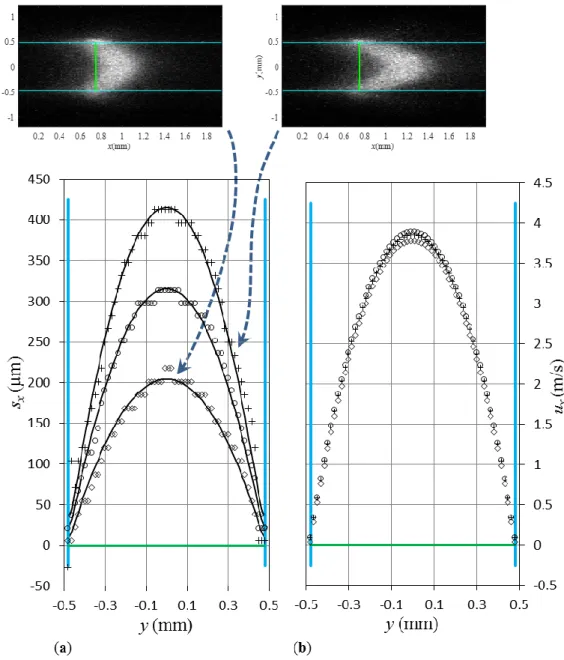
Fig. 6: MTV data of helium flow with Ly 960 32 µm , pin102.8kPa, pout 101.8kPa,
294K
T , Kn2.59 10 5 and D2/1,2 1.34 10 m s5 2 -1
.
(a) Experimental displacements sxexp( , )y tk at t1 50μs(◊); t2 80μs(o) ; t3 100μs(+); reconstructed displacements s y tx( , )k (─).
(b) Reconstructed velocity profiles u y tx( , )k at t (◊); 1 t (o); 2 t (+). 3
The mean velocity in the channel section can be estimated from the velocity profiles extracted in the mid-plane of the rectangular cross-section, in order to be compared to the mean velocity deduced from the flowrate measurements described in Section 3.2. The Reynolds number is of the order of Re35 and in this laminar flow regime, the estimated hydrodynamic entry length is about 3 mm, which ensures that the flow is fully developed in the tagged region located 10 cm downstream from the channel entrance. The velocity distribution in a fully
19
developed and steady laminar Poiseuille flow in a rectangular channel can be analytically calculated [69]. It allows to calculate the ratio a between the mean velocity v
2 2 ( , 0) y y L x L x y
u
u y z dy L in the symmetry plane (at z0) of the section and the mean velocity in the cross-section :2 2 2 2 2 2 1 ( , 0) 1 ( , ) y z y z L x Ly y v L L x L Ly y z u y z dy L a u y z dy dz L L
. (13)In the case of the present channel with an aspect ratio L Ly z 1 5, the calculation yields 1.1428
v
a .
From the flowrate measured by timing the draining of the balloon, the mean velocity at the central part of the channel is calculated as
, b x flowrate v y z V u a t L L , (14)
where t is the time for totally draining the balloon. This value is compared to the velocity data obtained from an integration of the MTV reconstructed velocity profiles shown in Fig. 6 -b: 2 , 2 , ( , 0) y y L x MTV L x MTV y u u y z dy L
. (15)It should be noted that in spite of the molecular diffusion in the z-direction, the velocity profile obtained from the experiments corresponds to the velocity profile in the central plane (
0
z ) of the section, as the aspect ratio of the section leads to a flat profile in the z-direction in the central part of the section (Fig. 7). During the short delay between tagging and measure, the diffusion in the z-direction only affects a region where the velocity is not z-dependent. The length of the tagged region increase in z-direction is given by:
2 2
0 2/1,2
( ) 2
z
d t d D t (16)
with d0 is the initial length corresponding to the laser diameter. Therefore, at the longest delay
used in this study, tk 130µs, dz do not exceed 60 µm. Consequently, the velocity profile is
measured at the central part of channel 3 500 z Lz 3 500, where the velocity gradient in
20
Fig. 7: Theoretical velocity field within the channel cross-section of aspect ratio 1/5, calculated from the model of (Spiga and Morini 1994). The velocity is normalized by its value at the center of the
section.
From the flowrate measurements, the calculated mean velocity in the symmetry plane of the section is ux flowrate, 2.49 0.09 m s, considering an expanded uncertainty with a coverage factor k2, whereas the mean velocity computed from the three MTV displacements profiles are 50µs , 2.49 m s x MTV u , 80µs , 2.58 m s x MTV u and 100µs , 2.56 m s x MTV
u . The maximal relative deviation obtained between the three MTV data and their average value ux MTV, 2.54 m s is 2 % and the deviation between ux MTV, and ux flowrate, is 2 %, which is reasonable for this kind of imaging velocimetry technique generally characterized by a few percent accuracy [58, 70]. Similar results have been obtained with a flow of argon (Fig. 8) at a mean pressure
100.7 kPa
mean
p seeded with acetone with a molar fraction
20.15.21
Fig. 8: MTV data of argon flow with Ly 960 32 µm , pin101.6kPa, pout 99.8kPa, T294K,
5
2.29 10
Kn and D2/1,2 7.47 10 m s 6 2 -1.
(a) Experimental displacements sxexp( , )y tk at t1 50μs(◊); t2 80μs(o) ; t3 100μs(+); reconstructed displacements s y tx( , )k (─).
(b) Reconstructed velocity profiles k( ) x
u y at t (◊); 1 t (o); 2 t (+). 3
The influence of the number of basis functions used for the decomposition of the velocity profile in Eq. (6) is now discussed. Considering the plane symmetry of the problem, only even basis functions (polynomials) are considered, according to Eq. (12). The introduction of odd polynomial would generate an asymmetric shape of the velocity profile. The displacements measured in helium flow at atmospheric pressure (Fig. 6-a) are processed using three decompositions. In the first case, the velocity is decomposed as u yx( )U0U y2( ); in the second case a fourth order contribution is added: u yx( )U0U y2( )U y4( ) and in the third
22
case a sixth order contribution is also considered: u yx( )U0U y2( )U y4( )U y6( ). The shape of the reconstructed velocity profiles are compared to the analytical solution of the Navier-Stokes equation in a normalized form in Fig. 9. The extracted mean velocities are not dependent on the number of basis function used. In the first case (diamonds) the velocity is reconstructed with a high accuracy, and adding higher order polynomials does not significantly modify the results. This result was foreseen, as in the present study the expected velocity profile at the central part of a quite flat rectangular channel, is very close to a parabola. Consequently, the decomposition in U and 0 U y are sufficient to correctly 2( ) reconstruct the velocity profile, but Fig. 9 demonstrates the robustness of the method on real experimental data and shows that additional terms do not reduce the accuracy of the extraction. This is a very interesting observation in view of analyzing more complex and a priori unknown velocity fields, for which higher order terms can play a significant role.
Fig. 9: Reconstruction velocities from MTV displacement (helium flow from Fig. 6-a), using a velocity decomposition (◊)u yx( )U0U y2( ); (×)u yx( )U0U y2( )U y4( ); (□) u yx( )U0U y2( )U y4( )U y6( ). Each represented profile results from averaging three
profiles corresponding to displacements measured at 50 µs; 80 µs and 100 µs (Fig. 6-a). (−) Comparison with Poiseuille theroretical profile.
-0,2 0 0,2 0,4 0,6 0,8 1 1,2 -0,5 -0,3 -0,1 0,1 0,3 0,5 ux (y )/ ux (0) y (mm)
23
4.2. Velocity profiles at sub-atmospheric pressure
At atmospheric pressure, the molecular slip at the wall due to diffusion was not very significant. This molecular slip is increased with a higher diffusion effect. A dimensionless tracer diffusivity can be introduced, writing Eq. (1) in a dimensionless form, in order to quantify this effect:
ˆ ˆ ( ) ²ˆ * ˆx x ˆ²x s s u y D t y (17)
In Eq. (17), ˆt t tk , yˆy Ly , ˆux u tx k Ly and ˆsx sx Ly, where t is the time between k
tagging and interrogation. 2 2/1,2
* k y
D t D L represents the ratio of the MTV experiment duration to the characteristic time of the tracer diffusion. In Fig. 6, for helium flow at atmospheric pressure, D* was ranging from 7.27 10 4 to 1.45 10 3 when t was varied k
between 50 and 100 µs. In Fig. 8, for argon flow at atmospheric pressure, D* was ranging from 4.05 10 4 to 8.11 10 4 when t was varied between 50 and 100 µs. By decreasing the k
pressure to sub-atmospheric values, higher dimensionless diffusivity are obtained, with a resulting higher molecular slip at the wall: 1.04 10 3D* 2.71 10 3 for argon flow at
42.35 kPa
mean
p and 1.31 10 3 D* 3.92 10 3 for helium flow at pmean52.7 kPa.
Results obtained in argon flows at pmean42.35 kPa are shown in Fig. 10. The molar fraction of acetone in the mixture is
2 0.23. An initial image is taken immediately after the laser pulse, thereafter snapshots of delayed images are successively recorded between50 µs
t and 130 µs with a 20 µs time-step. The displacement profiles obtained in this configuration are plotted in Fig. 10-a. Each of them exhibits a fourth-order polynomial shape and an artificial slip increasing with time is observed. The inherent dispersion of these profiles,d, due to both the molecular diffusion of the tagged molecules and the experimental uncertainties, is defined by
/2 2 2 0 0 2 2 /2 1 ( , ) ( , ) ( , ) y y L d x k k k y L s y t a S y t a S y t dy L
, (18)and is typically one decade smaller than the displacement amplitude s sx(0)s Lx( y 2), as shown in Fig. 10-d.
24
Fig. 10: MTV data of argon flow with Ly 944 32 µm , pin42.7 kPa, pout 42.0kPa, T294K,
5
5.38 10
Kn and D2/1,2 1.86 10 m s5 2 -1
.
(a) Experimental displacements sxexp( , )y tk at t1 50μs(◊); t2 70μs(o); t3 90μs(+);
4 110μs
t (×); t5 130μs (□); reconstructed displacements (─).
(b) Reconstructed velocity profiles at t (◊); 1 t (o); 2 t (+); 3 t (×); 4 t (□); overall averaged profile (5 ▬). (c) Area averaged displacement versus time (♦); best linear fit (─).
(d) Dispersion of the displacement profile normalized by the displacement amplitude (♦).
The velocity profiles u y tx( , )k computed by applying the reconstruction method are displayed in Fig. 10-b and are in very good agreement. Even at a sub-atmospheric mean pressure, the reconstruction is still very efficient since: (i) the displacement profiles are quite well
25
approached by the basis functions (solid lines in Fig. 10-a); (ii) the obtained velocity profiles are close to each other, exhibiting a dispersion of the velocity at the channel center lower than 3 %; (iii) the mean velocity computed directly from the linear time evolution of the average displacement (Fig. 10-c) as predicted by Eq. (5) shows a deviation with the mean velocity computed from the velocity profile (solid blue line in Fig. 10-b) lower than 2 %.
Fig. 11: Comparison between reconstructed velocity profile from Fig. 10-b (−)
and velocity profile extracted without reconstruction, simply obtained from the displacement data of Fig. 10-a at t4 110μs divided by t (4 - -) and fitted by a polynomial function.
From MTV data of argon flow with pin42.7 kPa, pout 42.0kPa, T 294 K.
The obtained reconstructed velocity profile shown in Fig. 10-b is compared in Fig. 11 to a velocity profile obtained without reconstruction, i.e. directly deduced from the displacement data of Fig. 10-a taken at t4 110μs, divided by t and smoothed by a polynomial function. 4
For the conditions of these experimental data, the Knudsen number is lower than 10-4 and the actual velocity at the wall should be zero, as correctly reproduced by the reconstructed velocity profile: the solid blue line intersects the measured position of the wall, represented by vertical solid dark blue line in Fig. 11, at ux0. On the contrary, it can be observed that if spanwise diffusion effects are not properly taken into account by using the reconstruction method, an artificial significant slip at the wall is erroneously evidenced, as shown by the dotted red line. In addition, the velocity in the center of the channel is slightly overestimated,
26
while it is underestimated for 0.15 mm y 0.4 mm. In the case of Fig. 11, the artificial slip is 9.1 % of the velocity in the channel axis (y0), whereas it is reduced after reconstruction to 0.8 %. Similar results are obtained from the displacement data obtained at each time
50,70,90,110,130 s
i
t : an artificial slip equal in average to 5.5 % of the center velocity is reduced to nearly zero, thanks to the reconstruction method, as shown in Fig. 10-b.
Experiments have also been conducted with a lighter background gas, helium, at a mean pressure pmean 52.7 kPawith
20.22. As shown in Fig. 12, the measured displacement profiles (Fig. 12-a), recorded between 30 µs and 90 µs with a 15 µs time-step, exhibit larger slips at the wall, highlighting a more pronounced diffusion effect. However, the dispersion d remains small, with values lower than 7 % of the displacement amplitude (Fig. 12-d). The application of the velocity reconstruction method, independently implemented for each measured displacement profile, provides coherent velocity profiles, as shown in Fig. 12-b. The mean flow velocity computed from the reconstructed profiles deviates less than 2% from the mean velocity extracted from the mean displacement shown in Fig. 12-c, using Eq. (5).27
Fig. 12: MTV data of helium flow with Ly 944 32 µm , pin53.1kPa, pout 52.3kPa,
294K
T , Kn5.03 10 5 and D2/1,2 3.88 10 m s5 2 -1
.
(a) Experimental displacements sxexp( , )y tk at t1 30μs(◊); t2 45μs(o); t3 60μs(+); t4 75μs(×);
5 90μs
t (□); reconstructed displacements (─).
(b) Reconstructed velocity profiles u y tkx( , )k at t1 (◊); t ( o ); 2 t (+); 3 t (×); 4 t (□); 5 overall averaged profile (▬).
(c) Area averaged displacement versus time (♦); best linear fit (─).
28
Finally, the averaged velocity profiles measured by MTV in the two previous cases (i.e. argon and helium flows) are compared to the predictions of Navier-Stokes equations in the continuum regime in Fig. 13. A good agreement is observed. Velocity profiles are compared in a normalized form since the pressures at the channel ends is not precisely known. This comparison, however, allows validating the shape of the reconstructed velocity profile, the capability of MTV to accurately capture the velocity magnitude being already demonstrated by successful comparisons with the flowrate measurements (Section 4.1).
Fig. 13: Measured velocity profiles: argon flow (×) and helium flow (◊) extracted from the blue solid lines in Fig. 10-b and Fig. 12-b, respectively, compared to Navier-Stokes predictions (▬).
5 Conclusion
µMTV is a promising tool for investigating the hydrodynamics of gas microflows, but the few recent experimental analysis using µMTV by direct phosphorescence [44] or by photoproduct fluorescence [57] show that Taylor dispersion is significant for Poiseuille gas flows in microchannels and leads to non-parabolic displacement profiles. In these two recent studies, the dimensionless tracer diffusivity, D*D2/1,2t L2y, where t is the time between tagging and interrogation, is particularly high, of the order of 4 10 3, due to the millimetric or sub-millimetric depth of the channel and to the low flow velocity. This effect can also be observed in liquid flows within smaller microchannels, as described in [60] where D* is of the order of
3
29
short delay between tagging and interrogation leads to a low dimensionless diffusivity, of the order of 5
5 10 [65]. When in addition the characteristic lengths are centimetric [35], the dimensionless diffusivity is even lower, of the order of 7
5 10 .
In the present paper, it has been demonstrated that the displacement of tagged molecules resulting from the hydrodynamic motion of the career gas was affected by molecular diffusion, and that this effect was significant for microscale gas flows, even in the continuum regime, and could lead to erroneous measurement of the velocity profiles if it was not taken into account during the data post-processing. However, it is possible to accurately extract the velocity profiles from the displacement profiles, using an appropriate post-processing method which takes into account the diffusion effect, and does not require any a priori assumption on the shape of the velocity profile. This reconstruction method has been successfully validated on experimental data from µMTV by direct phosphorescence. In experimental conditions for which the macroscopic velocity at the wall should be totally negligible, a significant molecular slip was experimentally observed at the wall. After post processing of the slipping displacement profile using the reconstruction method, the velocity profile was obtained and it was found that the velocity at the wall was zero, as theoretically expected. The mechanism responsible for a molecular slip -without any macroscopic velocity slip- at the wall has been explained.
The comparison of MTV results with flowrate measurements have shown a deviation of a few percent, and the extracted velocity profiles were in good agreement with Navier-Stokes based calculations. This investigation demonstrates the capacity of MTV to capture local velocity in confined flows with a good accuracy, even in the vicinity of the walls. Although the reconstruction method becomes inaccurate for high values of D*, typically higher than unity, it was numerically demonstrated [62] that it is still efficient when D* is of the order of 101. For such values, with the experimental setup described in the present paper, Knudsen numbers of the order of 2 10 2could be reached, which corresponds to the slip flow regime. This result, coupled with the present experimental validation of the data processing technique for lower values of D , confirms that MTV could be a promising technique to achieve the * challenging problem of local velocity measurement in rarefied regimes, and to provide a direct measurement of the slip at the wall. To reach this goal, additional research, currently in progress, aims at improving the quality of MTV images at low pressure, i.e. for higher Knudsen numbers.
30
Acknowledgements This research obtained financial support from the European
Community's Seventh Framework Program (FP7/2007-2013) under grant agreement no 215504, from the Fédération de Recherche Fermat, FR 3089, and from the Project 30176ZE of the PHC GALILEE 2014 Program. The latter is supported by the Ministère des Affaires Etrangères et du Développement International (MAEDI) and the Ministère de l’Enseignement Supérieur et de la Recherche (MENESR).
References
[1] I. Gerken, J.J. Brandner, R. Dittmeyer, Heat transfer enhancement with gas-to-gas micro heat exchangers, Applied Thermal Engineering, 93 (2016) 1410-1416.
[2] L.N. Cattafesta, M. Sheplak, Actuators for active flow control, Annu. Rev. Fluid Mech., 43 (2011) 247-272. [3] J. Gomez, R. Groll, Pressure drop and thrust predictions for transonic micronozzle flows, Phys. Fluids, 28 (2016) 022008.
[4] C.-J. Lu, W.H. Steinecker, W.-C. Tian, M.C. Oborny, J.M. Nichols, M. Agah, J.A. Potkay, H.K.L. Chan, J. Driscoll, R.D. Sacks, K.D. Wise, S.W. Pang, E.T. Zellers, First-generation hybrid MEMS gas chromatograph, Lab Chip, 5 (2005) 1123-1131.
[5] Y. Xu, J.-T. Lin, B.W. Alphenaar, R.S. Keynton, Viscous damping of microresonators for gas composition analysis, Appl. Phys. Lett., 88 (2006) 143513.
[6] S. Nakaye, H. Sugimoto, Demonstration of a gas separator composed of Knudsen pumps, Vacuum, 125 (2016) 154-164.
[7] S. An, N.K. Gupta, Y.B. Gianchandani, A Si-micromachined 162-stage two-part Knudsen pump for on-chip vacuum, IEEE J. Microelectromech. Syst., 23 (2014) 406-416.
[8] K.M. Kovach, M.A. LaBarbera, M.C. Moyer, B.L. Cmolik, E. van Lunteren, A. Sen Gupta, J.R. Capadona, J.A. Potkay, In vitro evaluation and in vivo demonstration of a biomimetic, hemocompatible, microfluidic artificial lung, Lab Chip, 15 (2015) 1366-1375.
[9] C. Niu, Y.-z. Hao, D. Li, D. Lu, Second-order gas-permeability correlation of shale during slip flow, SPE Journal, 19 (2014) 786-792.
[10] S. Colin, Rarefaction and compressibility effects on steady and transient gas flows in microchannels, Microfluid. Nanofluid., 1 (2005) 268-279.
[11] F. Sharipov, Data on the velocity slip and temperature jump on a gas-solid interface, J. Phys. Chem. Ref. Data, 40 (2011) 023101.
[12] N. Miyoshi, K. Osuka, I. Kinefuchi, S. Takagi, Y. Matsumoto, Molecular Beam Study of the Scattering Behavior of Water Molecules from a Graphite Surface, The Journal of Physical Chemistry A, 118 (2014) 4611-4619.
[13] S. Colin, Gas microflows in the slip flow regime: a critical review on convective heat transfer, J. Heat Transf.-Trans. ASME, 134 (2012) 020908.
[14] W.-M. Zhang, G. Meng, X. Wei, A review on slip models for gas microflows, Microfluid. Nanofluid., 13 (2012) 845-882.
[15] G.L. Morini, Y. Yang, H. Chalabi, M. Lorenzini, A critical review of the measurement techniques for the analysis of gas microflows through microchannels, Exp. Therm. Fluid Sci., 35 (2011) 849-865.
[16] P. Perrier, I.A. Graur, T. Ewart, J.G. Méolans, Mass flow rate measurements in microtubes: from hydrodynamic to near free molecular regime, Phys. Fluids, 23 (2011) 042004.
[17] T. Ewart, P. Perrier, I. Graur, J.G. Méolans, Mass flow rate measurements in gas micro flows, Exp. Fluids, 41 (2006) 487-498.
[18] J. Pitakarnnop, S. Varoutis, D. Valougeorgis, S. Geoffroy, L. Baldas, S. Colin, A novel experimental setup for gas microflows, Microfluid. Nanofluid., 8 (2010) 57-72.
[19] J. Maurer, P. Tabeling, P. Joseph, H. Willaime, Second-order slip laws in microchannels for helium and nitrogen, Phys. Fluids, 15 (2003) 2613-2621.
[20] S. Colin, P. Lalonde, R. Caen, Validation of a second-order slip flow model in rectangular microchannels, Heat Transfer Eng., 25 (2004) 23-30.
[21] E.B. Arkilic, K.S. Breuer, M.A. Schmidt, Mass flow and tangential momentum accommodation in silicon micromachined channels, J. Fluid Mech., 437 (2001) 29-43.
[22] S. Varoutis, V. Hauer, C. Day, S. Pantazis, D. Valougeorgis, Experimental and numerical investigation in flow configurations related to the vacuum systems of fusion reactors, Fusion Eng. Des., 85 (2010) 1798-1802.