1 Annotating mobile phone location data with activity purposes using machine learning algorithms
Feng Liua, Davy Janssensb, Geert Wetsb, Mario Coolsc
a,b
Transportation Research Institute (IMOB), Hasselt University, Wetenschapspark 5, bus 6, B-3590, Diepenbeek, Belgium
c
TLU+C (Transport, Logistique, Urbanisme, Conception) 1, Chemin des Chevreuils Bât B.52/3 4000 Liège, Belgium
E-mail address: [email protected] (F. Liu), [email protected] (D. Janssens),
[email protected] (G. Wets), [email protected] (M. Cools)
a
Corresponding author: Tel: +32 0 11269125 fax: +32 0 11269199 Manuscript
2
Abstract
Individual human travel patterns captured by mobile phone data have been quantitatively characterized by mathematical models, but the underlying activities which initiate the movement are still in a less-explored stage. As a result of the nature of how activity and related travel decisions are made in daily life, human activity-travel behavior exhibits a high degree of spatial and temporal regularities as well as sequential ordering. In this study, we investigate to what extent the behavioral routines could reveal the activities being performed at mobile phone call locations that are captured when users initiate or receive a voice call or message.
Our exploration consists of four steps. First, we define a set of comprehensive temporal variables characterizing each call location. Feature selection techniques are then applied to choose the most effective variables in the second step. Next, a set of state-of-the-art machine learning algorithms including Support Vector Machines, Logistic Regression, Decision Trees and Random Forests are employed to build classification models. Alongside, an ensemble of the results of the above models is also tested. Finally, the inference performance is further enhanced by a post-processing algorithm.
Using data collected from natural mobile phone communication patterns of 80 users over a period of more than one year, we evaluated our approach via a set of extensive experiments. Based on the ensemble of the models, we achieved prediction accuracy of 69.7%. Furthermore, using the post processing algorithm, the performance obtained a 7.6% improvement. The experiment results demonstrate the potential to annotate mobile phone locations based on the integration of data mining techniques with the characteristics of underlying activity-travel behavior, contributing towards the semantic comprehension and further application of the massive data.
Keywords activity-travel behavior, sequential information, machine learning algorithms, feature
selection techniques, mobile phone location annotation.
1. Introduction
1.1. Problem statement
Nowadays, mobile phones are often used as an attractive option for large-scale sensing of human behavior. They provide a source of real and reliable data, allowing automatic monitoring of the call and travel behavior of individuals. In-depth studies to discover mathematical laws that govern the key dimensions of human travel, such as the travel distance and the time spent at different locations have been conducted in the domain of physics (e.g. González et al., 2008; Song et al., 2010). Using call location records, these studies provide a modeling framework capable of capturing general features of human mobility.
However, despite the disclosure of these general features, previous studies do not provide further insights into the motivation or the activity behaviour behind the identified travel patterns. In general, most of the current research on mobile phone location data has mainly focused on spatial and temporal dimensions (e.g. Calabrese et al., 2011). The behavioural aspects associated with the travel patterns, such as travel mode and daily activities being performed at the locations, are still in a less-explored stage. Due to growing concerns over matters of confidentiality, location data provided by phone operation companies usually do not have contextual information, leading to a wide gap between the raw mobile phone data and the semantic interpretation of the trajectories. As a result, there is a long way to go from individual travel patterns identified from mobile phone data up to high level behavioural mobility knowledge, capable of supporting
3 management decisions that are related to activity behaviour. This is exactly the challenge which lies ahead, and if a methodology can be found which helps to bridge this gap, the potential applications using the semantically enriched phone data are immense. They include, among others, the provision of activity tailored services in the mobile phone environment (e.g. Huang et al., 2009; Hwang & Cho, 2009), mining individual life styles and activity preferences in urban planning (e.g. Becker et al., 2011), and inferring people’s travel motivations in activity-based transportation modelling in which the daily activities of individuals and households have long been hypothesized to be the key determinants of travel demand (e.g. Axhausen & Gärling, 1992). 1.2. Related state-of-the-art
So far, there have been a number of research efforts that tried to derive the activities being pursued at a location from GPS-based (Global Positioning Systems) data or from multi-modal data collected by smart phones. The essential part in the annotation on GPS-based trajectories is the use of geographic information. This process starts with the decomposition of continuous GPS sample points into a sequence of stops, where the individual has adjourned for a minimum period of time doing activities, and moves that represent the sample points between two consecutive stops. The stops are then compared with a geographic map by overlapping them in space, in order to find interesting places specified by users, such as hotel and touristic sites, which are relevant to the application of the trajectories.
The geographic information based annotation process has received considerable attention during the past years (e.g. Bohte & Maat 2009; Du & Aultmanhall 2007; Moiseeva et al., 2010; Schuessler & Axhausen, 2009), but still is confronted with various limitations. (i) The process demands a high level of precision of geometric data, e.g. longitude and latitude, in order to gain a good match between the movement points and the exact positions of interesting places. For collecting such information, tools such as GPS are needed, which are expensive in terms of battery consumption (e.g. Montoliu & Gatica-Perez, 2010). (ii) Linking a GPS-based trajectory to detailed geographic information on all communities, offices, shopping and leisure area in a studied region needs a lot of computational efforts (e.g. Zheng et al., 2010). (iii) The process does not only entail a cost-related and computational drawback, but also a methodological issue: indeed, the result of this (geographical) methodology is location-specific and the quality of the annotation process depends per definition on the study area, which makes the process not transferable towards other regions. (iv) The geographically matched location alone may not reveal a particular motivation as to why a person is observed there. For instance, the person could go to a shopping area with the purpose of shopping, working or just having a lunch, depending on other factors, e.g., the visit frequency to the location and the regular time and duration of the stay (e.g. Alvares et al., 2007; Reumers et al., 2012). (v) Apart from the above economical and methodological limitations, the geographical matching of exact GPS positions of an individual raises a high level of privacy concerns, as some of the specific places visited by the person may be highly privacy-sensitive (e.g. Eagle & Pentland, 2009).
Recently some of the above limitations have been addressed by building the annotation process on data from multi-modal sensors equipped on smart phones, independent of geographic information (e.g. Laurila et al., 2012). This annotation process, which we shall call ‘multi-modal-sensing-data-annotation’, was comprised of two stages. In the first stage, a smart framework was designed to efficiently collect users’ movement traces from a combination of GPS data and data from other sensors, e.g. Wi-Fi and accelerometer (Montoliu & Gatica-Perez, 2010). For each individual, the collected points were then clustered into a number of places, each of which was represented by an identification number rather than geographic positions of the cluster points. In
4 the second stage, the semantic meaning of these places was inferred, by using contextual information from the sensors and phone applications, e.g. data from Wi-Fi, accelerometer, Bluetooth, phone call, message logs, media player, and so on, as opposed to a detailed map. In this stage, GPS data was not available to researchers, as the intention was to explore the possibility of location annotation by other types of data, in order to address privacy concerns. Various machine learning methods have been proposed in the second stage, with different sets of features being extracted from the sensing data as inputs (e.g. Chon et al., 2012; Huang et al., 2012; Montoliu et al., 2012; Sae-Tang et al., 2012; Zhu et al., 2012). These studies have achieved promising prediction performance without the need of additional geographic information and GPS coordinates. They also found that across the various types of sensing data, the features which characterize the temporal aspects of a place, e.g. the relative visit frequency and average time spending at the place, play a critical role. Nevertheless, looking to this entire annotation process starting from raw smart phone location traces, while it eliminates the necessity for a map, it still partly relies on GPS data for the identification of visited places in the first stage. Thus this annotation process as a whole does not fully address the privacy issue. In addition, while these annotation methods mainly focus on choosing efficient classification models and relevant features for a high prediction rate, none of them have conducted a post-processing analysis to examine how the predicted results perform in the context of daily activity sequences which are under a certain sequential constraint. An in-depth analysis into the classification errors for potential improvement of the inference is also absent in these studies.
1.3. Research contributions
Extending the current research on semantic annotation of people’s movement traces, and in the meantime addressing the above mentioned limitations, our study proposes a new approach which is based on data derived from simple mobile phones and which uses existing data mining techniques combined with the characteristics of underlying activity-travel behavior which originates the traces. The fundamental research contributions of this work can be situated in the following areas. (i) The proposed method is based on spatial and temporal regularities as well as sequential information inherent to human activity-travel behavior. (ii) It is independent of additional sensor data and map information, thus significantly reducing data collection costs and relatively easily transferable to other regions. (iii) Along with the use a set of machine learning algorithms, a post-process has been developed to enhance the inference performance. (iv) A set of extensive experiments and an in-depth analysis on the annotation results have been conducted to evaluate the effectiveness of the proposed method and to identify the classification errors, using mobile phone data collected from 80 people’s real life over a period of more than one year. (v) Compared to precise GPS points, the wide coverage of a cell ID in a GSM network allows the behavioral annotation process to reduce the level of privacy worries considerably, thus well addressing this issue which has been paramount considerations over the collection and use of the massive data.
The rest of this paper is organized as follows. Section 2 describes the mobile phone data and Section 3 details the annotation process. A set of extensive experiments are subsequently conducted in Section 4 and an in-depth analysis on the experiment results is carried out in Section 5. Finally, Section 6 ends this paper with major conclusions and discussions for future research.
5 The mobile phone data was collected by a European mobile phone company for billing and operational purposes. It consists of full mobile communication patterns of 80 users over a period of more than one year between 2009 and 2011, recording the location and time when each user conducts a call activity, including initiating or receiving a voice call or message, enabling us to reconstruct the user’s time-resolved call location trajectories. The locations are represented with coordinates of base stations (cells) in a GSM network; each of the stations has a wide coverage ranging from a few hundred square meters in metropolitan to a few thousand in rural areas, controlling our uncertainty about the user’s precise location. The users along with mobile phone number and cell IDs, are all anonymized. Table 1 illustrates typical call records of an individual identified as ‘310001620’ on Thursday, April 29th
, 2010.
Table 1 The typical call records of an individuala
UserId CellID Day Time Duration Description Direction
310001620 10057 29042010 12:08 22 Voice call Outgoing
310001620 10057 29042010 13:51 0 Voice call Missed call
310001620 10057 29042010 15:18 48 Voice call Outgoing
310001620 10086 29042010 18:40 0 Message Incoming
310001620 10091 29042010 21:38 0 Message Outgoing
a The columns from the left to the right respectively represent the user, the base station where the user is located, the
day, time and duration (in minutes) of the call activity, the type of this activity including voice call and message, and the direction including incoming, outgoing and missed calls for ‘voice call’ and incoming and outgoing for ‘message’.
Among all the users, 11032 distinct calling locations were detected. From the locations, 259 (2.3% in total) have been labeled with activities performed at these places and they are used as the ground-truth data for training and evaluating our models. All the labeled locations are classified into 5 activity types, including ‘home’, ‘work/school’, ‘non-work obligatory’, ‘social visit’ and ‘leisure’, accounting for 29%, 30%, 12%, 15% and 14% of the total training data, respectively. The ‘home’ activity encapsulates all time spending at home, while the ‘work/school’ refers to all work or school related activities outside home. The ‘non-work obligatory’ includes activities such as bringing/getting people, shopping and personalized services; these activities along with ‘work/school’ activities are expected to subject to a high level of spatial and temporal constraints (e.g. Frusti et al., 2002). Regarding the remaining two activity types, the ‘social visit’ refers to all visit activities to friends, colleagues or family members and the ‘leisure’ accommodates all recreational activities such as indoor or outdoor sports, eating or drinking at restaurants, and tour. These two activity types are assumed to have lowest priority among all daily activities and they exhibit highest level of flexibility in spatial and temporal choices (e.g. Arentze & Timmermans, 2004).
If different types of activities are conducted in a same location for a particular individual, the most frequent activity is assigned to this location, such that each location is uniquely linked to an activity type for the individual.
3. Annotation Process
3.1 Overview of the approach
The approach to annotate mobile phone data that is proposed in this paper integrates basic knowledge about human travel behavior into the location annotation process, and extracts the information from mobile phone call records into concrete variables. Findings related to daily
6 activity-travel decision making process are incorporated. Hannes et al. (2008) underlined the routine and automated features of this decision making process. People do not generally plan their everyday activities consciously on a day to day basis; but rather rely on fixed routines or scripts executed during the day without much consideration. This generates a high level of spatial stability and temporal periodicities in activity-travel behavior (e.g. Hannes et al., 2010; Spissu et al., 2009) as well as a certain sequential order of the activities (e.g. Wilson, 2008). Evidence also suggest that activity-travel behavior differs across various time periods of a day (e.g. Schlich & Axhause, 2003), that weekday behavior generally does not extend into the weekend (e.g. Buliung et al., 2008), and that holidays have a non-ignorable impact on daily activity-travel behavior (e.g. Cools et al., 2010).
On the other, the spatial and temporal recurrences of the locations can be adequately reflected in movement traces left behind by mobile phone users. Although a selective number of calls during a few days do not provide much information about a user’s daily activity-travel routines, a long period of call records could reveal sufficient clues on the visit frequency of a call location and the regular time and duration of the stay. The temporal and spatial constraints of the call locations, stemming from the characteristics of various activities which are performed in their own daily, weekly or monthly rhythms, can thus suggest the possible activities carried out at the locations, enabling annotation at the third dimension, i.e. travel motives (activities), in addition to the spatial and temporal dimensions.
The annotation process consists of four steps. First, a set of variables is defined which profile each call location in the spatial and temporal dimensions, with an emphasis on how to segment a day. Next, feature selection techniques are applied to choose the most effective variables. Upon the selected variables, a set of classification models and an additional ensemble method to integrate these prediction results are employed. In the last step, all the predicted activities are filled into the daily sequences of trips for each individual, and a post-process is developed to enhance the annotation performance based on sequential constraints of the activities.
3.2. Variable definition
For each individual, first, all distinct locations, where the individual has conducted at least a call activity over the entire data collection period, are identified. Assume of N unique locations for a selected individual. Then, at each call location Li (i=1,…,N), a set of variables from two perspectives is defined: the call behavior and the underlying activity-travel behavior. The call behavior defines variables that directly reflect the characteristics of phone communication behavior, consistent with the features extracted from call and message records in the ‘multi-modal-sensing-data-annotation’ process. The underlying activity-travel behavior, however, tries to approximate the spatial and temporal profiles of a location by using call data. For instance, the call frequency ‘CallFreqR’ describes how often a call activity is conducted at a location; by contrast, the visit frequency ‘VisitFreqR’ reveals how often the location is accessed, regardless of the number of calls that the user has made at each visit. A second major difference lies in activity duration: the call duration ‘CallDuration’ is simply the length of the time a call activity lasts; but the duration for each visit ‘VisitDuration’ is defined as the time interval between the earliest and latest time of a sequence of consecutive call activities made at the location. If a visit is marked by only a single call activity during the entire period of the visit, the visit duration is zero if the activity is a missed call or message and equal to the call duration if a voice call is conducted. Based on existing research on activity-travel behavior, variables in each of these two perspectives are defined according to the following 4 categories: spatial repetition, temporal periodicity,
7 weekday-weekend-holiday differences, and day segments. All the variables are presented in Table 2.
Table 2 Definition of temporal variables
Underlying activity-travel behavior Call behavior
Spatial repetition Spatial repetition
VisitFreqR: the visit frequency at the
location divided by the total visit frequencies to all locations by the individual.
CallFreqR: the call frequency at the location divided by the total
call frequencies at all locations by the individual.
[VoiceCall/Message]FreqR: the variable ‘CallFreqR’ is
segmented between voice call and message, respectively.
[Incoming/Missed/Outgoing]CallFreqR: the variable ‘VoiceCallFreqR’ is divided into incoming, missed and outgoing calls.
[Incoming/Outgoing]MessageFreqR: the variable ‘MessageFreqR’ is divided into incoming and outgoing messages.
Temporal variability Temporal variability
TotalVisitDurationR: the total duration of
all the visits to the location divided by the duration of visits to all locations by the individual.
[Earliest/Latest]VisitTime a: the earliest and latest call time of all call activities at the location, respectively.
AverageVisit[StartTime/ EndTime], VarianceVisit[StartTime/EndTime]:
the average and variance of the first and last call time over all visits at the location, respectively.
[Longest/Average/Variance]VisitDuration:
the longest and average duration of all visits to the location, and the variance of the duration, respectively.
TotalCallDuration: the total call duration of all call activities
made at the location by the individual.
CallInterval[Max/Ave]: the maximum and average time interval
between 2 consecutive call activities at the location, respectively.
[Average/Variance]CallTime: the average and variance of call
time of all call activities made at the location, respectively.
[Longest/Average/Variance]CallDuration: the longest, average
and variance of call duration of all calls made at the location, respectively.
Weekday-weekend-holiday Weekday-weekend-holiday
VisitFreqR[Week/Weekend/Sun/Sat/Holid ay],TotalVisitDurationR[Week/
Weekend/Sun/Sat/Holiday]: the variables
‘VisitFreqR’ and ‘TotalVisitDurationR’ at weekdays, weekend, Sunday, Saturday, or public holidays, respectively.
CallFreqR[Week/Weekend/Sun/Sat/Holiday],
TotalCallDurationR[Week/Weekend/Sun/Sat/Holiday], VoiceCallFreqR[Week/Weekend/Sun/Sat/Holiday], MessageFreqR[Week/Weekend/Sun/Sat/Holiday]:
the variable ‘CallFreqR’, ‘TotalCallDuration’. ‘VoiceCallFreqR’ and ‘MessageFreqR’ at weekdays, weekend, Sunday, Saturday, or public holidays, respectively.
Day segment Day segment
VisitFreqR[1/ …/ m] b,
TotalVisitDurationR[1/…/m]: the variable
‘VisitFreqR’ and ‘TotalVisitDurationR’ are segmented during different time periods of a day, respectively.
CallFreqR[1/ …/ m], TotalCallDurationR[1/ …/ m], VoiceCallFreqR[1/ …/ m], MessageFreqR[1/ …/ m]: the
variable ‘CallFreqR’, ‘TotalCallDuration’, ‘VoiceCallFreqR’ and ‘MessageFreqR’ are segmented during different time periods of a day, respectively.
a The symbol [] represents different variables, such as [Earliest/Latest]VisitTime for variables ‘EarliestVisitTime’
and ‘LatestVisitTime’.
b Each day is divided into m segments, and m is determined by the method described in the following.
With regard to the definition of day segments, it should be noted that heterogeneous activity-travel patterns have been observed for the different time periods of a day (e.g. Schlich & Axhausen, 2003). Yet, different definitions (in terms of the cutting points) of day segments or time periods have been adopted in literature, depending on the context of the study area. Instead
8 of making such an a-priori assumption, Janssens (2005) proposed a method which estimates the cutting points of the day segments from empirical data. However, his method is limited by assuming an equal length of time intervals, which might not be generally true as the length of the segments may vary. In this paper, we enhance this estimation method by iteratively choosing the most significant cutting point at each previously obtained segment. The resultant cutting points may not generate equal intervals, but delimit the largest differences in the distribution of various activity types among these intervals.
In order to reduce the computational burden, only hourly based cutting points are examined in this study, but a more detailed division, e.g. per 30 minutes, could be applied as well. The exact time of each call activity is first converted into hours, for instance, the time of a call made between 9am and 9:59am is discretized into 9am. Next, if multiple calls are made within one hour at a same location, they are aggregated into one observation indicating that the person has performed the corresponding activity during this hour on this particular day.
The segment process starts with a full day of 24 hours (from 0 to 23pm), and each hour is examined independently. An hour under investigation divides the day into two time intervals, for instance, at 9am, the two obtained intervals are 0-9am and 9am-23pm respectively. A contingency table is then constructed; in which these two time intervals and the activity types are the row and column variables respectively, and the total frequency of the aggregated observations over all individuals that fall into the corresponding time intervals and the activity classes are the cell values. Thus, each cell value represents the total times that people have been seen doing a certain activity at the relevant time interval. A Chi-square statistics is subsequently computed for this contingency table that is corresponding to the selected hour.
After the Chi-square statistics are obtained for each of the 24 hours respectively, the hour with the largest value across all the 24 statistics is chosen as the first cutting point, denoted as
r
1. Thishour divide the day into two segments between 0 and
r
1 as well as betweenr
1 and 23. Thisprocedure is iterated for each of the newly created segments, until further cutting does not gain considerable differences or until a predefined number of segments is reached.
3.3. Feature selection
Given the relatively large number of variables compared with the small labeled training dataset, over-fitting is a potential concern. To overcome this possible problem, prior to running the classification models, feature selection techniques are performed to reduce the number of predictor variables actually used by the models. Two methods, namely filter and wrapper, which have proved their effectiveness in the ‘multi-modal-sensing-data-annotation’ process, are chosen for feature selection. The filter method looks at each feature individually and then selects the one that has a high correlation with the target variable, but a low correlation with the features that have already been selected (Hall, 1998). In contrast, the wrapper method conducts a search for an optimal subset of features by using the classification model itself, and cross-validation is used to estimate the accuracy of the learning model for each feature subset (Kohavi & John, 1997). 3.4. Machine learning
A group of state-of-the-art machine learning methods, including Multiclass Support Vector Machine (SVM) (Keerthi et al., 2001), Multinomial Logistic Regression (MNL) (le Cessie & van Houwelingen, 1992), Decision Tree (DT) (Quinlan, 1993), and Random Forest (RF) (Breiman, 2001), have been adopted in this study. These methods have shown comparative performance among well-established algorithms for multi-category classification problems as shown by
9 various studies (e.g. Arentze & Timmermans, 2004; Zheng et al., 2010) as well as by the existing ‘multi-modal-sensing-data-annotation’ process.
The differences among these algorithms mainly lie in the way the classification task is approached, the structure of the learning function, and the procedure for determining the optimal function parameters (e.g. Liao et al., 2012). As each learning algorithm has its strengths and limitations, it is often a challenge to find a single classifier that performs best for a particular learning task (e.g. Kwon & Sim, 2012). Integrating two or more algorithms together to solve a problem could utilize the strengths of one method to complement the weaknesses of another (e.g. Caruana & Kotsiantis, 2006; Kotsiantis, 2007). This motivates the development of a fusion process in which the 4 individual model prediction results for each call location are considered as predictors, and the observed activity types remain as the dependent variable. The relation between the predicted and observed results can then be formulated as a classification problem, which again can be solved by a classification model. In this fusion process, the use of a classification model as opposed to majority voting rules, is due to the fact that the learning model predicts the probabilities of different possible outcomes of the dependent variable and these probability values will be subsequently fed into the post-process for further analysis.
3.5. Post-process
While regular machine learning algorithms offer an effective technique for annotating each single location, it discards the details of activity ordering and transitions embedded in daily activity-travel patterns. When the annotated locations are filled into an individual’s diary, the daily activity sequence should have a certain sequential constraint to follow.
It has been widely acknowledged that the choice of activities is dependent on the preceding activity engagement (e.g. Joh et al., 2007; Wilson, 1998). For instance, during one particular working day, it is highly probably that the combination of having breakfast, travel and working is observed together. On the contrary, if a sports activity is carried out in the morning, there is a small chance that it is performed again in the evening. The interdependencies of daily activities have been considered as a crucial factor in activity-travel decision making, such as on the sequential choice of activities and locations (e.g. Janssens et al., 2005) and on trip chains which include several short-stop activities on the way to home or work places (e.g. Kasturirangan et al., 2002).
By considering the sequential information, the activity locations which are accessed by an individual on the same day are viewed and tackled as a whole, rather than an isolated participation in activities. However, such sequential information which involves at least two different locations is not always available for each day. For instance, people may stay at home an entire day, engaging only in a single (home) activity. This is particularly true with mobile phone location data as people do not necessarily make calls when going to a new location, leading to daily movement trajectories not fully revealed by their call records. In these cases, we turn to the typical user behavior at different time of a day: the prior probability distribution of activities at different time. Assume P(aj|X) is the probability of activity
a
j performed at a locationj
based on the observed temporal variables
X
, derived in the preliminary inference model. By applying Bayesian methods, we predict the posterior probability of this activity based onX
and the call timet
, i.e., P'(aj|X,t). Sincet
is involved in the conditional part, this probability is more discriminative and informative than P(aj| X), and it can be estimated fromP(aj|X) and the prior probability distribution P(aj|t) (See formula 3).
10 3.5.1. Rationality of the post-process
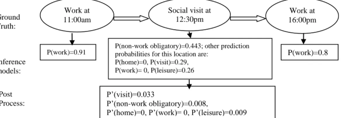
The post-process takes the preliminary inference results as well as the sequential knowledge and the prior activity distribution as inputs, and aims to generate an improved prediction result. The process is comprised of two components: transition probability-based enhancement and prior probability-based enhancement. This method has shown its effectiveness in the study by Zheng et al. (2010), which aims at improving machine learning prediction results on transport modes using GPS data. This process can be illustrated by the daily trajectory of a user depicted in Figure 1. According to the call records in the example, the user has conducted the sequence of activities of work → social visit → work at the corresponding call time on that day. But the prediction from the inference models would be work → non-work obligatory → work; thus a prediction error occurred. On this occasion, if a location (the 2rd location in this example) has a prediction probability (e.g. 0.443) which is less than a threshold T1 (i.e. 0.72 in our experiment), it is assumed that it has a very high probability of being a false inference. The post-process is then applied to this location to improve its prediction in the following manner. (i) If there is a second activity location in the daily sequence which is adjacent to this first one, which has a probability exceeding a certain threshold T2 (e.g. 0.9), it is considered to be a possibly correct prediction and thus used to fix the potentially false inference of the first location (including backward and forward), using the transition probability-based enhancement. (ii) Otherwise, if no other activity locations appear in the neighboring areas which are estimated with a high probability, the prior probability-based enhancement method is performed to improve the prediction based on the call time at this location.
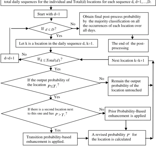
After recalculation, the activity with the maximum enhancement probability is selected as the prediction result of the revised location on that particular day. As a location may be repeatedly visited on multiple days, the multiple days’ enhanced prediction results are combined by majority voting rules as the final post-processing classification for the location. With the appropriate threshold T1 and T2, it is more likely to correct the false prediction while maintaining accurate inference results. This process flow is demonstrated in Figure 2.
Figure 1. Daily call location trajectory of a user
Inference models: P(work)=0.91 Work at 11:00am Social visit at 12:30pm Work at 16:00pm P(work)=0.8 3
P(non-work obligatory)=0.443; other prediction probabilities for this location are:
P(home)=0, P(visit)=0.29, P(work)= 0, P(leisure)=0.26
P’(visit)=0.033
P’(non-work obligatory)=0.008,
P’(home)=0, P’(work)= 0, P’(leisure)=0.009 Ground
Truth:
Post Process:
11
Figure 2. Post-process
3.5.2. Transition probability-based enhancement
The sequential information is represented in a transitional probability matrix between different activities, e.g. 55 in this study. Let
a
i anda
j be the activities performed at previous locationi
and current locationj
respectively,a
i,
a
j
1
,
2
,...
5
. Let Tr(aj|ai) be the transitional probability from activitya
i to activitya
j, which can be calculated from the training data as follows. 5 1 ) | ( ) | ( ) | ( ak a a F a a F a a Tr i k i j i j ) | (a aF j i is the frequency of activity
a
j followed bya
i. The probability of location jbeing annotated as activitya
j conditioned by the activitya
i at previous locationi
can be recalculated as: ) | ( ) | ( ) | ( 0 a a Tr X a P X a P j j j i (1) Yes Yes Yes Transition probability-based enhancement is applied. Yes No No No No If the output probability ofthe location PT
1?
For each individual, fill the annotated locations into daily sequences of movement; assume D total daily sequences for the individual and Total(d) locations for each sequence d, d=1,…,D.
Next location k=k+1
Prior Probability-Based enhancementis applied Beginning of the post-process
Obtain final post-process probability by the majority classification on all the occurrences of each location over all days.
If there is a second location next to this one and has P T
2 ?
A revised probability P' for the location is calculated If dD?
Remain the output probability of the location untouched Start with d=1
Let k is a location in the daily sequence d, k=1.
IfkTotal(d)? d=d+1
The end of the post- processing
12 Here 0( | )
X a
P j stands for the modified probability; P(aj|X)is the output of the inference model.
Based on formula 1, however, the modified probability of a location is biased towards frequently visited activity locations e.g. home and work/school places, as transitions to these places are likely to be higher than to other less visited places. Consequently, most of the locations under such modification will be redirected to these two types of activities. To avoid this, the previous transition probability is divided by the frequency of the current activity
a
j, resulting in the probability of Qr(aj|ai) , 5 1 5 1 ) | ( ) | ( ) | ( ) | ( ak ak a a F a a F a a F a a Qr k j i k i j i j The 0( | ) X a P j can be revised as P'(aj|X), ) | ( ) | ( ) | ( ' a X P a X Qr a a P j j j i (2)In this user’ case in Figure 1, since the transition probability Qrfrom work to non-work obligatory activity is very small, after the modification, P'(nonworkobligatory) (e.g. 0.008) drops behind P' visit( ) (e.g. 0.033), we get the visit activity as the revised result.
3.5.3. Prior Probability-Based Enhancement
By applying the Bayesian rule, as well as by assuming that
X
is independent oft
, the posterior probability P'(a |X,t)j of activity
a
j conditioned onX
and call timet
can be decomposed as follows. ) ( ) | ( ) | ( ) ( ) ( ) ( ) ( ) ( ) | ( ) ( ) ( ) | ( ) ( ) ( ) ( ) | , ( ) , ( ) , , ( ) , | ( ' a P t a P X a P t P X P a P a P t P t a P a P X P X a P t P X P a P a t X P t X P t X a P t X a P j j j j j j j j j j j j (3) The prior probabilities P(a |t)j and P(aj) can be summarized from the training data:
5 1 5 1 ) ( ) ( ) ( , ) | ( ) | ( ) | ( a ak k a F a F a P t a F t a F t a P k j j k j j . Here, F(a |t)
j is the frequency of activity
a
j occurring at timet
and F(aj) the frequency ofa
j at all time. P(aj|X) can be approximated by the probability generated by the inference models.13 However, as acknowledged in the work (Zheng et al., 2010), from the theoretic perspective, there are two weak assumptions concerning the above calculation. One is the substitution of P(a |X)
j by the inference model, the other goes to the assumption of the independence between
X
andt
, Nevertheless, based on the equation 3, the preliminary model prediction probability is complemented by the prior activity distribution) ( ) | ( a P t a P j j at time
t
. 4. Case studyIn this section, a set of experiments, adopting the proposed annotation approach and using the mobile phone data described in Section 2, are presented and the results of these experiments are discussed in detail. The first step in the experiments is the identification of the optimal day segment points, followed by the extraction of the temporal variables for each of the call locations. Next, feature selection techniques and classification models (including the ensemble method) are applied. The differences in prediction performance are analyzed. In the last step, both the transition matrix and the activity distribution are derived from the mobile phone data. Based on these probabilities, a post-process is then developed to enhance the prediction results. The performance of the post-process is further evaluated.
4.1. Day segments
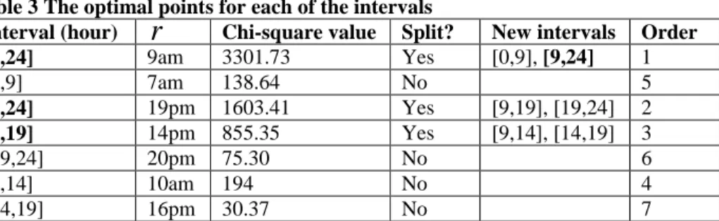
Table 3 lists the optimal points for each of the intervals, based on the previously described method. The first cutting point over an entire day was found at 9am, generating 2 new intervals of 0-9am and 9am-24pm. This search process was iterated for each of the two newly obtained intervals. If the largest Chi-square value over all potential points of an interval was lower than a predefined threshold, i.e. 200 in this experiment, this search stops. The columns in Table 3 respectively represent the current interval under investigation, the optimal cutting point
r
, the corresponding Chi-square value, the fact whether or not the interval is split (if this is the case then two new segments are formed), and finally, the order of the optimal points according to the significance of the Chi-square values.Table 3 The optimal points for each of the intervals
Interval (hour)
r
Chi-square value Split? New intervals Order [0,24] 9am 3301.73 Yes [0,9], [9,24] 1 [0,9] 7am 138.64 No 5 [9,24] 19pm 1603.41 Yes [9,19], [19,24] 2 [9,19] 14pm 855.35 Yes [9,14], [14,19] 3 [19,24] 20pm 75.30 No 6 [9,14] 10am 194 No 4 [14,19] 16pm 30.37 No 7Figure 3 shows the evolution of the Chi-square statistics of the previously identified optimal points, in which the positions in the first 3 orders yield much higher values than the remaining ones. From the 4th position on, the statistics starts to decline sharply. Thus the first 3 optimal points are extracted and 4 segments were generated as a result: (i) 0-8:59am (night period), (ii) 9am-13:59am (morning period), (iii) 14am-18:59pm (afternoon period) and (iv) 19pm-23.59pm (evening period).
14
Figure 3. The evolution of Chi-square statistics of the optimal points
After each day is segmented into the 4 different periods, all the variables defined in Section 3.1 are then obtained and used as the candidates for subsequent feature selection and machine learning. Weka, an open-source Java application which consists of a collection of machine learning algorithms for data mining tasks (Witten et al., 2011), is used for the implementation. 4.2. Feature selection and machine learning
4.2.1. Model evaluation criterion
The 10-fold cross-validation method is used to train and evaluate the models, in which the original training dataset is randomly divided into 10 parts, each part being held alternatively as the validation set and the remaining parts combined as the training data. An overall prediction rate can be obtained by averaging the 10 classification rates of the validation data. The evaluation metric is then defined as
dataset training original in the locations total of Number i set ion in validat locations annotated correct of Number = Accuracy 10 1 i
4.2.2. Performance of individual classifiers
Table 4 lists the prediction results of the different individual classifiers, running on each of the variable subsets which are chosen by each of the two feature selection techniques (filter and wrapper methods). For each of the models, the results with the best two parameter settings are presented. In addition, the prediction by using all candidate variables is also conducted as a base-line reference.
The above analyses are built on the features of call locations which are drawn from the perspectives of both underlying activity-travel behavior and call behavior. In comparison, an extra set of experiments is also carried out which only uses the users’ call behavior.
15
Table 4 Prediction accuracy of each of the individual classifiers (%)
Classification
Models Parameters
Both underlying activity-travel behavior and Call
behavior Call behavior Feature Selection All Variables Feature selection All Variables Filter Wrapper Filter Wrapper
SVM-poly c=100,degree=1 63.50 59.26 56.93 59.85 59.49 57.30 c=10, degree=1 62.41 59.12 58.14 59.85 58.76 59.85 SVM- RBF c=100, Gamma=0.01 65.69 a 56.57 59.85 60.58 58.39 59.85 c=10, Gamma=0.01 56.20 55.90 58.76 52.92 52.91 51.82 MNL C=1 64.23 68.98 a 63.50 62.77 65.69 60.58 C=10 63.50 62.04 62.41 58.39 61.31 62.77 DT N=3 60.22 60.95 59.12 55.47 60.95 56.20 N=4 60.95 a 60.58 59.12 58.76 59.85 56.57 RF N=0 65.33 66.06 a 64.60 62.77 63.50 62.04 N=1 64.96 64.68 63.19 66.06 61.31 57.66
a the highest prediction accuracy for each model.
Table 4 indicates that models running on a subset of variables, chosen by both feature selection techniques, perform better than models operating on all predictors available, with an average improvement of 2.13% for filter methods and 0.85% for wrapper methods. This demonstrates the importance of feature selection techniques when handling a relatively large number of predictors given a small training set. However, there is no general conclusion on which feature selection method is better in this experiment. SVM works better with the Filter method; while the performance of DT and RF does not vary much with these two feature selection techniques. On the other hand, MNL gains a remarkable improvement of 4.8% when it is supplemented with the Wrapper method.
When the different classification models are compared, it was observed that MNL generates the best results with a 68.98% accuracy, followed by an accuracy of 66.06% and 65.69%, for RF and SVM. DT is lagging behind with a prediction accuracy of 60.95%. Both RF and DT use the same classification algorithm, e.g. C4.5 in this experiment, but with different designs. RF is based on the theory of ensemble learning that allows the algorithm to learn both simple and complex interactions between predictors. This algorithm is particularly appealing in the presence of unbalanced classes of the target variable or datasets with more predictors relative to the number of observations (e.g. Statnikov et al., 2008), which is the case in this study.
A third comparison was carried out between the variables drawn from the aspects of both activity-travel and call behavior, and the ones simply characterizing the call behavior. In most cases, the prediction accuracy using the combination of activity-travel and call behavior is higher than that with solely the call behavior. The average accuracy increases by 2.96% and 1.20% for filter and wrapper methods, and 2.09% when all variables are included. This underlines the importance of the additional variables defined based on underlying activity-travel behavior. 4.3. Important predictors
The different feature selection techniques yield divergent optimal subsets of features. Table 5 presents 8 variables which were picked up by the multiple selection processes. The distributions of two representative variables including ‘VisitFreqRWeek’ and ‘TotalVisitDurationRSun’ are
16 illustrated in Figure 4. Figure 4(a) shows that, as expected, home and work/school places have a much higher level of average access during weekdays than the locations for remaining activities, including social visit, non-work obligatory and leisure activities. While regarding the time spending on Sunday as described in Figure 4(b), a different grouping of the activities is observed, including a considerably higher level of home activities, middle level of social visit and work/school activities, and low level of non-work obligatory and leisure activities.
Table 5 Important variables Underlying activity-travel behavior VisitFreqRWeek TotalVisitDurationRSun VarianceVisitEndTime VarianceVisitStartTime AverageVisitEndTime Call behavior AverageCallTime IncomingMessageFreqR MessageFreqR3
Figure 4. Distribution of variables ‘VisitFreqRWeek’ (a) and ‘TotalVisitDurationRSun’ (b)
Note: Activity types are represented as follows. H: home, V: social visit, W: work/school, O: non-work obligatory, and L: leisure.
4.4. Results of fusion models
Each of the classifiers with the best parameter performance in Table 4 is selected for the integration. The 4 individual classifiers are also employed as the fusion models to predict the combined results. Table 6 presents the prediction results, revealing that a fusion model does not necessarily outperform the individual models; the performance depends on the choice of the fusion models. For instance, MNL obtains a 68.98% accuracy as an individual classifier, while it achieves 69.71% when used as the fusion model running on the combination of all the 4 individual model results. This accuracy drops when other classifiers are used as the fusion model for this integration.
17
Table 6 Prediction accuracy of various fusion models (%)
Classification Models Fusion Models SVM- RBF MNL DT RF SVM- RBF MNL DT RF X X 62.4 63.1 62.8 60.6 X X 66.4 68.25 a 64.6 65.3 X X 66.05 68.98 a 66.05 68.98 a X X X 64.60 67.15 64.23 65.69 X X X 64.96 67.15 67.15 66.06 X X X 64.60 66.06 66.05 64.23 X X X 64.60 68.25 a 64.96 62.04 X X 67.15 64.60 69.71 a 68.24 a X X 64.96 61.68 64.96 64.23 X X 67.15 66.42 63.14 64.60 X X X X 67.52 69.71 a 65.69 62.04
a The prediction with accuracy above 68%; X: the corresponding model is chosen.
4.5. Post-process
4.5.1. Transitional matrix
Similar to the temporal variables, the transition matrix is also built for weekdays and weekend separately as well as for different periods of a day. As the typical operation time of various activities differs across a day, the transition between them is also likely to be different. The identification method of the optimal cutting points is the same as previously described, except with two substitutions. The first is related to the time intervals. For each potential dividing point, two intervals but three scenarios are obtained depending on the occurring time of the two concerned activities in the transition. The first scenario occurs when both activities take place in the first interval. The second scenario is the situation where the first activity takes place in the first interval and second activity in the second. Finally the third scenario occurs when both activities take place in the second interval. The second difference lies in the structure of contingency table. The row and column variables of this contingency table are the three scenarios and all the possible outcomes of activity transitions, i.e. 25 in this experiment. The cell values of the contingency table represent the transition frequency of the corresponding activities in the corresponding scenario.
Given the small size of the training set and the relative large number of cells in the contingency table, only the first significant cutting point was selected. In this case this cutting point was identified at 18pm. Under this time division, the largest difference in the distribution of activity transitions was found among the three corresponding scenarios: transition within the interval of 0-17:59pm, transition from the interval of 0-17:59pm to the interval of 18-23:59pm, and transition within the interval of 18-23:59pm. Table 7 shows the transition matrix in the first scenario during weekdays. As expected, for the probability Tr(a |a)
i
j , the highest values are dominated by the transitions to either home or work/school activities. With Qr(aj|ai), however,
the dominance of these two activities is reduced by their high frequency, and transitions to other less represented activities are exposed. This can be manifested by the high likelihood of transitions from home to non-work activity locations and from social visit to second social visit locations.
18
Table 7 Transition matrix in the first scenario during weekdays Previous
Activity
Current Activity
Transition probability Tr Transition probability Qr Home Social Visit Work/ School Non-Work
Leisure Home Social Visit Work/ School Non-Work Leisure Home 0.008 0.017 0.883 a 0.032 0.061 0.002 0.023 0.060 0.066 a 0.059 Social Visit 0.197 0.080 0.701 a 0.000 0.022 0.057 0.113 a 0.047 0.000 0.021 Work/School 0.546 a 0.081 0.328 0.010 0.036 0.159 a 0.114 0.022 0.019 0.035 Non-Work 0.700 a 0.000 0.300 0.000 0.000 0.204 a 0.000 0.020 0.000 0.000 Leisure 0.797 a 0.051 0.153 0.000 0.000 0.232 a 0.072 0.010 0.000 0.000
a The maximum probability Tr and Qr for each row.
4.5.2. Activity distribution at different time
Regarding the activity distribution, a distinction is also made between weekdays and weekend. Figure 5(a) shows the weekday activity distribution at each hour P(aj|t) and Figure 5(b) displays the distribution of this variable relative to the overall distribution of the concerned activity P(aj). A remarkable deviation is observed between these two figures: Figure 5(a) shows that either home or work/school activities dominate the activity distribution throughout the day, whereas Figure 5(b) reveals that the most likely activity shifts across various types as the day unfolds.
Figure 5. Absolute activity distribution at each hour (b) and relative activity distribution at each hour (b)
4.5.3. Selection of threshold T1 and T2
Based on the results in Table 6, two fusion models were selected to test the post-process: a MNL fusion model built on the integration of all the 4 individual models and a RF fusion model running on the combination between this model and MNL.
In order to choose the appropriate threshold T1 and T2 , an analysis is conducted on the correlation between the inference probabilities obtained from the fusion models and the percentage of the correct and false predictions. Figure 6 demonstrates this relationship for the MNL and RF fusion models. Both models exhibit a common feature: when the inference probability is below a certain value, e.g. at the crossing point which is 0.72 in Figure 6(a) and 0.8 at Figure 6(b), the number of false prediction is higher than that of the correct ones. Thus, 0.72 and 0.8 are respectively chosen as T1. The value T2 is set as 0.9. Above this value, the corrected prediction rate is 69.7% and 66.4% respectively for both models.
19
Figure 6. Correlation between the percentage of the correct/false prediction and the inference probabilities from MNL fusion model (a) and RF fusion model (b)
4.5.4. Post-processing results
The results by the post-process are presented in Table 8, along with the prediction results before this enhancement. An overall improvement of 4.4% and 7.6% for the MNL fusion model and RF fusion model are achieved. When the results across various activities are examined, it was noted that the post-process particularly works on less representative activity types, e.g. non-work obligatory, leisure and social visit activities, as indicated in the column ‘Differences’. This could be due to the fact that the machine learning algorithms usually favor majority classes if the classification accuracy is used as the model evaluation criterion, while the post-process puts equal weights on all classes of the target variable.
To examine the performance of each of the two enhancement methods, this post-process is repeated with a RF fusion model, by using each of these enhancement methods independently to revise a weak prediction. For the transition probability-based enhancement, a 73.7% accuracy was obtained, while with the prior probability-based enhancement, an prediction rate of 75.2% was gained. Due to the small training set, many labeled locations appear as a single known event on a day, thus the sequential information is not available on these days. With a large-scale dataset, the transition matrix would become more capable of representing typical user activity behavior. It thus is believed that the transition probability-based enhancement method and the post-process as a whole would bring a greater improvement to current experimental results.
Table 8 Prediction result comparison between before post-process and after that (%) Fusion
Model
Activity types
Overall accuracy Home Visit Work/
School Non-Work Leisure MNL Before post-process 91.3 47.4 80.9 37.5 45.7 69.7 After post-process 91.3 55.3 82.0 59.3 48.6 74.1 Differences 0 7.9 1.1 21.8 2.9 4.4 RF Before post-process 91.3 52.6 74.2 53.1 37.1 69.0 After post-process 91.3 60.5 79.8 78.1 51.4 76.6 Differences 0 7.9 5.6 25.0 14.3 7.6
20
5. Analysis on the final prediction results
The detailed prediction results over all activity types by the RF fusion model after post-processing are presented in Table 9, showing a large variation in this model’s performance across the activities. This difference mainly results from the different degree of spatial and temporal regularities exhibited by the activities. For instance, rhythms at home, work/school and non-work obligatory activity places are more stable and as a result these locations are better predictable, with the accuracy of 91.3%, 79.8% and 78.1% respectively. By contrast, locations for recreation purposes are only 51.4% recognizable. The remaining social visit activities show a middle level of predictability of 60.5%. Overall, a prediction accuracy of 76.6% has been achieved.
Notwithstanding the promising results, a certain degree of misclassification exists for each of the activity types. This prompts for a further examination into the activity locations and identification of potential reasons for the prediction errors.
Table 9 Prediction results across different activity types(%)
5.1. Home
Home locations are mainly characterized with high visit frequencies both during weekdays and weekend days. They exhibit the highest level of spatial and temporal regularities in people’s daily life. However, still 7 homes are missed out from the correct identification, of which 5 have very low weekday visit frequencies of 10%, i.e. less than 1 in 10 trips during weekdays ending at home.
Two factors could explain the unusually less visited homes. First, the corresponding individuals may be engaged more in outdoor activities and thus spend more time outside home. Or even if they stay home, they may make fewer calls than expected from average call behavior, leading to the home visit frequency less represented by call records. Second, some of these locations can be a second home for individuals who already have a home at a different location. Two out of these 5 individuals are observed to have two documented homes in the training set. While their second home are visited occasionally, their main home are used more regularly and predicted correctly. 5.2. Work/school activities
Like home, work/school locations are also profiled by highly routine visits, but these two types of locations differ mainly in terms of the time of the visits. While home accommodates a major part of time spending at night as well as at weekend, especially on Sunday (see Figure 4(b)), most of work/school places are left empty during these times, but occupied during weekdays, especially in the morning and afternoon periods.
Out of all the work/school locations, 10.1% are predicted as social visit or non-work obligatory activity locations if they are visited less frequently during weekdays. Further investigation
Original activity Predicted activity Home Social Visit Work/ School Non-Work Leisure Home 91.3 3.8 1.2 2.5 1.2 Social Visit 15.8 60.5 7.9 10.5 5.2 Work/School 10.1 4.5 79.8 5.6 0 Non-Work 3.1 6.2 9.3 78.1 3.1 Leisure 2.8 14.3 14.3 17.1 51.4
21 discloses that all the corresponding individuals work/study at multiple places, and the occasionally visited locations are their additional work/school places.
The other 10.1% of all the work/school locations are mistaken as home, as they show high visit frequency at weekend. A representative of these individuals is ‘310001638’, who has two labeled work locations: the first one was visited at the rate of 32% and 0.2% during weekdays and on Sunday, respectively, and it was correctly identified. By contrast, the second one was visited at a high rate of 42% on Sunday, and it was thus wrongly predicted as home.
The above analysis suggests that the temporal work regime plays important role in differentiating a person’s work locations from home. While the majority of people work during weekdays and stay at home at weekend, certain minorities do not follow this trend. Instead, they shuttle on different working shifts, especially to weekend or night, generating distinct activity-travel patterns from the main stream of the population. This presents a challenge in distinguishing work locations from home.
5.3. Social visit activities
Social visit locations can be featured by a middle level of visit frequency during weekdays; if they are accessed lower than this level, they tend to be estimated as places for non-work obligatory or leisure purposes, if higher, they may be seen as home or work/school places. Causes of the limited predictability for this activity can be partially attributed to the underlying complex structure of an individual’s social network, in which various level of relationship exist, ranging from closed ones they visit regularly to the ones they just meet once in a while (e.g. Hidalgo & Rodriguez-Sickert, 2008). The different strength of social ties that an individual has with his/her friends, relatives or colleagues, could influence the frequency and the duration of their face-to-face contacts, potentially giving rise to variation in spatial and temporal features of the social visit locations.
5.4. Non-work obligatory activities
Among all the 5 activity types, non-work obligatory activities exhibit the lowest average level of visit frequency and duration. The misclassification for these activities can be partially explained by a combination of heterogeneity within this activity type. Although the various non-work obligatory activities share an overall lower level of visit frequency and duration, they are likely carried out at spatially independent locations and temporally varied preferences. For example, time for shopping displays a relatively larger variance and later shift than the time at places for services or picking up people.
5.5. Leisure activities
Leisure activities are often carried out in various places and at a flexible time schedule (e.g. Spissu et al., 2009); they have the lowest level of spatial and temporal regularities and thus are the most challengeable to predict.
An examination into the falsely predicted leisure locations points out two representative cases. The first one was visited at the rate of 36.3% during weekdays, particularly in the afternoon and evening periods. This location is the second most visited place for the concerned individual ‘310001605’, who has accessed this place 170 times across 337 survey days in total. Approximately every 2 days, he was observed at this location. This location is originally labeled as a restaurant, the temporal features of his/her call activities however signals a high likelihood that this person may work there instead of eating as a customer.