Constraints on the shallow elastic and anelastic structure of Mars from InSight seismic data

(1)

an author's https://oatao.univ-toulouse.fr/25961

https://doi.org/10.1038/s41561-020-0536-y

Lognonné, Philippe and Banerdt, W. B. and Pike, W. T... [et al.] Constraints on the shallow elastic and anelastic structure of Mars from InSight seismic data. (2020) Nature Geoscience, 13 (3). 213-220. ISSN 1752-0894

(2)

T

he Interior Exploration using Seismic Investigations, Geodesy and Heat Transport (InSight) mission landed on Mars on 26

November 2018 in Elysium Planitia1,2_{, 38 years after the end}

of Viking 2 lander operations. At the time, Viking’s seismometer3

did not succeed in making any convincing Marsquake detections, due to its on-deck installation and high wind sensitivity. InSight therefore provides the first direct geophysical in situ investigations of Mars’s interior structure by seismology1,4_.

The Seismic Experiment for Interior Structure (SEIS)5

moni-tors the ground acceleration with six axes: three Very Broad Band (VBB) oblique axes, sensitive to frequencies from tidal up to 10 Hz, and one vertical and two horizontal Short Period (SP) axes, cover-ing frequencies from ~0.1 Hz to 50 Hz. SEIS is complemented by

the APSS experiment6_{(InSight Auxiliary Payload Sensor Suite),}

which includes pressure and TWINS (Temperature and Winds for InSight) sensors and a magnetometer. These sensors monitor the

atmospheric sources of seismic noise and signals7_.

After seven sols (Martian days) of SP on-deck operation, with

seismic noise comparable to that of Viking3_{, InSight’s robotic arm}8

placed SEIS on the ground 22 sols after landing, at a location selected through analysis of InSight’s imaging data9_{. After levelling and noise}

assessment, the Wind and Thermal Shield was deployed on sol 66 (2 February 2019). A few days later, all six axes started continuous seismic recording, at 20 samples per second (sps) for VBBs and 100 sps for SPs. After onboard decimation, continuous records at rates from 2 to 20 sps and event records5_{at 100 sps are transmitted.}

Several layers of thermal protection and very low self-noise enable the SEIS VBB sensors to record the daily variation of the

17

_{, V. Lekic}

18

_,

A. Stott

4

_{, E. Stutzmann}

1

_{, S. Tharimena}

3

_{, R. Widmer-Schnidrig}

20

_{, F. Andersson}

5

_{, V. Ansan}

13

_,

C. Beghein

14

_{, M. Böse}

5

_{, E. Bozdag}

21

_{, J. Clinton}

5

_{, I. Daubar}

3

_{, P. Delage}

22

_{, N. Fuji}

1

_{, M. Golombek}

3

_,

M. Grott

_{, R. Weber}

32

_,

D. Banfield

38

_{, M. Wieczorek}

39

_{, C. Yana}

28

_{and P. Zweifel}

5

Mars’s seismic activity and noise have been monitored since January 2019 by the seismometer of the InSight (Interior Exploration using Seismic Investigations, Geodesy and Heat Transport) lander. At night, Mars is extremely quiet; seismic noise is about 500 times lower than Earth’s microseismic noise at periods between 4 s and 30 s. The recorded seismic noise increases during the day due to ground deformations induced by convective atmospheric vortices and ground-transferred wind-generated lander noise. Here we constrain properties of the crust beneath InSight, using signals from atmospheric vortices and from the hammering of InSight’s Heat Flow and Physical Properties (HP3_{) instrument, as well as the three largest Marsquakes detected}

as of September 2019. From receiver function analysis, we infer that the uppermost 8–11 km of the crust is highly altered and/ or fractured. We measure the crustal diffusivity and intrinsic attenuation using multiscattering analysis and find that seismic attenuation is about three times larger than on the Moon, which suggests that the crust contains small amounts of volatiles.

(3)

Sol 194–195 (LMST): VBB Z

12:00:00 18:00:00 00:00:00 06:00:00

Sol 194–195 (LMST): VBB N/S 12:00:00

14 Jun, 00:00 14 Jun, 06:00 14 Jun, 12:00 14 Jun, 18:00 15 Jun, 00:00

(2019)

(2019) 18:00:00 00:00:00 06:00:00 Sol 194–195 (LMST): VBB E/W 12:00:00 18:00:00 00:00:00 06:00:00 –5.0 –5.5 –6.5 Accel. (log(m s −2 Hz −1/2 )) Accel. (log(m s −2 Hz −1/2 )) –7.0 –7.5 –8.0 –8.5 –9.0 –9.5 –10.0 –6.0 –5.0 –5.5 –6.5 –7.0 –7.5 –8.0 –8.5 –9.0 –9.5 –10.0 –6.0 Accel. (log(m s −2 Hz −1/2 )) –5.0 –5.5 Frequency (Hz) 101 100 10–1 Frequency (Hz) 101 100 10–1 Frequency (Hz) 101 100 10–1 –6.5 –7.0 –7.5 –8.0 –8.5 –9.0 –9.5 –10.0 –6.0

Fig. 1 | Spectrograms of the vertical, north and east components of acceleration from 0.02 to 50 Hz versus lmst for typical sol 194–195. The spectrogram

includes data from both the VBB and SP seismometers in the bands where their respective noise is lowest: below 5 Hz, the acceleration shown is measured by the VBBs; above 5 Hz, it is measured by the SPs. Four events associated with bursts of energy in the 2.4-Hz resonances have been identified by the MarsQuake Service47_{(MQS) catalogue}27_{. Data were not returned for two 12-min periods on one SP axis.}

(4)

seismic noise at Mars’s surface, down to the lowest noise recorded so far by a seismometer on the surface of a terrestrial body, at periods between 5 and 20 s.

Figure 1 shows the spectrogram of a typical sol of seismic

data on Mars (sol 194–195), in the 0.02–50 Hz band. Starting at 17:00–18:00 lmst (local mean solar time), extremely low noise lev-els are observed until midnight. During the lowest-wind period, accelerations below 1.5 × 10–10_{m s}−2_Hz−1/2_{at 0.4 Hz are detected,}

corresponding to ~3 Å root mean squared ground displacement in a one-octave bandwidth. This is ~1/500 of the Earth Low Noise

Model10_{, allowing detection of events with a moment magnitude}

Mw ~ 1.8 lower than on Earth. The levels of noise are comparable to

those recorded by Apollo11_{on the Moon at 1 Hz (Fig.}₂_{), but much}

lower at longer periods. After midnight, the noise increases slightly until sunrise, and then rises rapidly with atmospheric boundary layer activity, from 7:00 to 16:00 lmst, still remaining below the Low Noise Model between 2 and 20 s. These three noise regimes, associ-ated with wind ranging from night-time laminar flow to daily tur-bulent flow, will probably provide new constraints on the Martian

Planetary Boundary layer12_{when better understood.}

Correlation analyses of SEIS with pressure and wind data (Supplementary Discussion 1) confirm the Martian environment as the key contributor to seismic noise, in line with prelanding

pre-dictions13–18_{. Observations (Supplementary Figs. 1–3 and 1–4 of}

Supplementary Discussion 1) suggest that long periods are domi-nated by ground deformation due to pressure perturbation and wind stresses, while shorter periods are dominated by lander-gen-erated noise excited by wind.

Subsurface constraints from atmospheric vortices and HP

3 The elastic properties of Mars’s near surface (upper 10–20 m) pro-vide information on geological processes that have shaped the landing site but are also required to fully understand the seismic noise. We derive a first elastic model using three independent seis-mic techniques at vertical scales varying from a few centimetres to ~10 m and at horizontal scales up to several tens of metres.

At a 5-cm scale, SEIS’s feet with their 2-cm spikes are in contact with the duricrust, a thin, weakly cemented layer about 1 cm below

unconsolidated soil2_{. From the modelling of resonant frequencies}

of the SEIS levelling system19_{, a local Young’s modulus of 47 MPa}

is inferred (Supplementary Discussion 2–1). This value is in agree-ment with geological inferences of a cohesive layer about 35% stiffer

than the material immediately below2_.

At a 1-m scale, the bulk seismic velocity of the regolith was constrained using travel-time measurements of hammer strokes

from HP3_hammering20_{, acting as a seismic source at 0.33 m depth.}

See Methods21,22_{and Supplementary Discussion 2–2 for details.}

Through precise knowledge of the HP3_{and SEIS clocks and}

averag-ing data from multiple hammer strokes, the travel time was

deter-mined to be 9.40 ± 2.68 ms over a distance of 1.11 m, yielding an

apparent P-wave velocity estimate of Vapp

P = 118 ± 34 m s−1.

At horizontal scales of 10–100 m (Supplementary Figs. 2–5), the near-surface material was probed using ground deformation caused by convective vortices (Supplementary Discussion 2–3), or ‘dust devils’ if made visible by their dust content, passing in the vicinity

of InSight and producing distinct pressure drops detected by APSS7_,

as well as vertical motion and ground tilt detected by SEIS (Fig. 3).

The ground velocity and pressure measurements23,24_{provide values}

for the ground compliance, computed as the ratio of the signal’s ground velocity to its correlated atmospheric pressure. Compliance is a function of wavelength, and thus can provide depth-dependent elastic properties of the subsurface15,16,23,24_.

Vapp

P and the ground compliance provide complementary

con-straints on properties of the upper regolith layer and the brecciated

bedrock beneath. Figure 4 presents the probability density

func-tion (PDF) of possible seismic structures of the topmost 10 m using

these constraints and assuming a near-surface compaction model25_.

The most probable models are generally consistent with the regional geological structure3_{, with V}

P ranging from 90 m s−1 at ~5 cm below

the surface to 145 m s−1_{at ~80 cm depth. This suggests that the}

degraded crater (Homestead Hollow) where SEIS is deployed is

filled largely with unconsolidated cohesionless sandy material2

with seismic velocities lower than those of previously considered

Mars analogues26_{. A compliance-only inversion (Supplementary}

Figs. 2–6) provides higher probabilities for stiffer regolith, but sam-ples a larger surface area.

Crustal seismic attenuation and diffraction

This first seismic structural analysis of Mars is based on the three best-recorded quakes until September 2019, occurring on sols 128, 173 and 235. Their amplitudes exceed 10–8_{m s}–2_Hz–1/2_{either below}

1 Hz (S0173a and S0235b) or above 1 Hz (S0128a). The complete

collection of seismic sources includes 171 other events4,27_with

smaller amplitudes.

The peak-to-peak vertical ground acceleration of S0128a is

about 8.5 × 10−7_{m s}–2_{in the 2–10-Hz bandwidth (Supplementary}

Figs. 1–9). Those of S0173a and S0235b are 3.5 × 10–8_{m s}–2

and 3.5 × 10–8_{m s}–2_{respectively in the 0.2–1-Hz bandwidth}

10–2

Earth (BFO)

Earth Low Noise Model Moon (Apollo) InSight on the deck (SP) 10–3 10–4 10–5 10–6 (m s –2 Hz –1/2 ) 10–7 10–8 10–9 10–10 10–11 0.01 0.1 1 Frequency (Hz) Probability 10 0.05 0.04 0.03 0.02 0.01 0

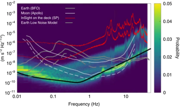
Fig. 2 | Statistical comparison of Martian, terrestrial and lunar seismic noise. The colour contours show the PDF of Martian vertical seismic noise measured by InSight VBB and SP during sol 194–195. They provide the fraction of time with respect to the total observation time. VBBZ and SP1 are shown for frequencies of <5 Hz and >5 Hz respectively. The red lines provide the seismic noise measured on the spacecraft’s deck by the SPs. The two lines represent the 16% and 84% percentile lines, which correspond to a 1σ Gaussian distribution. Grey lines are an example of

terrestrial seismic noise measured at Black Forest Observatory (BFO) in Germany. STS1 data were used for long-period (<2 Hz) noise statistics and STS2 data were used for shorter periods (>2 Hz). The two lines represent the 16% and 84% percentile lines. Dashed grey is the lowest noise for Earth from the Low Noise Model10_{. The white lines are an example of} lunar seismic noise measured during the Apollo seismic observation. The Apollo long-period seismometer was used for frequencies of <1 Hz and the short-period seismometer was used for frequencies of >1 Hz. In addition to the 16% and 84% percentile lines, the 2.5% percentile curve, which corresponds to the lower limit of the 2σ noise, is depicted in the figure to

show the lowest noise level on the Moon, which is most likely due to the instrument self-noise5,11_{. Finally, the black line is the theoretical instrument} noise curve for the VBB estimated from noise expected from each subsystem5_{. During the night, noise levels are smaller than the minimum} observed on the Moon, but in both cases these noise floors are close to those of the sensors in the 0.1–5-Hz bandwidth. The Moon is quieter than Mars in the daytime due to activity in the Martian atmosphere. Note also the extreme differences between Earth, Mars and the Moon due to the lack of the oceanic microseism.

(5)

(Supplementary Figs. 1–10 and 1–11). None have surface waves, suggesting a depth too large to excite them above the noise and/

or surface-wave scattering4_{. Their high signal-to-noise ratio,}

par-ticularly with respect to wind (Supplementary Discussion 1 and corresponding spectra, seismograms and wind/pressure records in Supplementary Figs. 1-8–1-11) enable us to (i) characterize attenuation and diffraction in the Martian crust and (ii) search for upper-crustal layering using the receiver function (RF) method to identify conversion of seismic waves during their propagation in the crust.

All three large events are dominated by long incoherent wave-trains. Polarization analysis reveals a high degree of polarization for only a small fraction of the time. Scattering is a possible can-didate to explain some of the signal characteristics. Scattering and attenuation properties are estimated from the S0128a, S0173a and S0235b records.

The S0128a signal is above the noise floor for frequencies of >2.5 Hz. The morphology of its seismogram is very similar to those

of Moonquakes28_{as illustrated in Fig.}_5b–c_{. The waveform is}

char-acterized by a stabilization of the ratio between the kinetic energies measured on the vertical and horizontal components, which is very reminiscent of high-frequency coda waves excited by small crustal

quakes on Earth29_{. Further examination, described in Supplementary}

Discussion 3, reveals two energy bursts, the first one being mostly visible above 6 Hz. Due to the lack of polarization, one cannot confi-dently identify the first burst as P and the second one as S. However, a simplified elastic radiative transfer calculation reproduces reason-ably well the two energy packets seen in the data for a hypocentral distance Δ = 530 km, VS= 3 km s−1 and VP/VS = √3. Furthermore,

the model shows that the signal between the tentative P and S arrivals is largely dominated by S waves, which offers an attractive explanation for the stabilization of the vertical-to-horizontal energy

partitioning ratio during the event. The absorption time of shear

waves (~80–85 s) yields an absorption quality factor Qi ~ 3,770–

4,006 at 7.5 Hz. In the event frequency band, the decay time appears fairly constant, so we may speculate that Qi ~ 503–534 at 1 Hz. The

diffusivity inferred from the data (D ~ 90 km2_s−1_{) depends}

strongly on the hypocentral distance, which is poorly determined.

For instance, with a distance of 375 km (found for tS− tP= 75 s,

VS = 2.5 km s−1 and VP/VS = 2, where tS and tP are the arrival times

of S and P), the diffusivity is reduced by a factor of 2. Whereas the inferred diffusivity is strongly dependent on the assumed quake location, the absorption time is not. Note, however, that only an apparent absorption has been derived, since the possible leakage of

diffuse energy from crust to mantle has been neglected30_.

Further constraints on attenuation have been gained through the analysis of S0173a and S0235b events. Both events contain signal above the noise floor in the range 0.2–0.9 Hz and show identifiable, coherent P and S pulses with approximately linear polarization. After each coherent arrival, the signal shows a coda with no charac-teristic polarization. The signal-to-noise ratios are higher than for S0128a and the events are located at roughly 1,720 km and 1,535 km

distances4_{. This suggests seismic waves propagating in a relatively}

transparent but attenuating Martian mantle before entering the regional crustal structure beneath InSight.

The observed long coda duration appears to be due to the interaction of teleseismic waves with a heterogeneous crust. Using a simple acoustic radiative transfer model in a waveguide geometry, we inverted for D and the intrinsic attenuation factor

Qi for S waves in the crust, based on the coherent S wave and its

coda (Supplementary Discussion 3). In spite of its simplicity the model takes leakage into account, which is key to obtaining a

reli-able estimate of absorption. The trade-off31_{between D and Q}

i is

studied in Supplementary Discussion 3. Our analysis suggests 0.2

–0.2

Pressure (Pa) Pressure (Pa)

–0.4 –0.6 0 0.2 –0.2 –0.4 –0.6 0 2 ×10–8 ×10–8 ×10–8 ×10–8 ×10–8 ×10–8 –2 Vertical (m s –2) Vertical (m s –2) Parallel (m s –2) Parallel (m s –2) Transverse (m s –2) Transverse (m s –2) –4 0 1 –1 0 1 –1 0 2 –2 0 5 –5 0 4 0 2 0 20 40 Time (s) Time (s) Data Vortex model Data Vortex model Sorrells's model 60 80 100 0 20 40 60 80 100 0 20 40 60 80 100 0 20 40 60 80 100 0 20 40 60 80 100 0 20 40 60 80 100 0 20 40 60 80 100 0 20 40 60 80 100

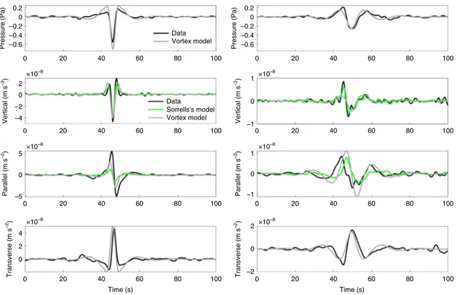
Fig. 3 | Pressure and seismic signature of two convective vortices compared with models. Data and models are filtered between 3 s and 20 s. The three seismic components and pressure data are well modelled using the vortex model14_{. The following parameters are assumed, respectively, for the short-} (long-) period events: dust devil radius of 3.5 m (6 m), core pressure drop of 11.5 Pa (14 Pa), closest approach distance of 7 m (14 m), vortex advection speeds of 4.5 m s−1_(2.5 m s−1_{), Young’s modulus of 200 MPa (300 MPa) and Poisson’s ratio of 0.22. The events are also well modelled using Sorrells’s} theory15,23_{with the same values for the Young’s modulus. Only the vertical compliance is used for the inversion.}

(6)

D ≥ 200 km2_s−1_{and Q}

i ≥ 800 at 0.5 Hz. The latter bound is roughly

one-third that reported for the dry megaregolith of the Moon in

the same frequency band32_.

Thanks to these three events, preliminary comparisons with the scattering and attenuation properties of the shallow part of the Earth and Moon can be made. The diffusivity of Mars ranges from 0 1 2 3 4 5 6 7 8 9 10 Depth (m) V_P regolith (m s–1₎ PDF (%) 0 1 2 3 4 5 6 7 8 9 10 Depth (m) 500 1,000 1,500 500 1,000 1,500 V_P bedrock (m s–1₎ 0 0.1 0.2 PDF (%) 0 0.5 1.0 Regolith Bedrock b 0 10 20 30 40 50 60 70 Frequency (%) 0 200 400 600 800 1,000 1,200 1,400 1,600 VP (m s–1) c 0 10 20 30 Frequency (%) 0 2 4 6 8 10 12 14 16 18 20 Regolith-to-bedrock transition (m) a d

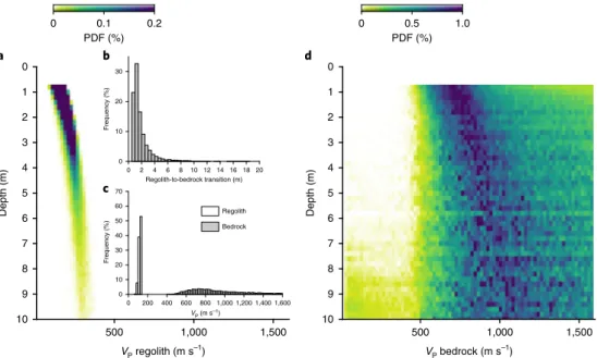
Fig. 4 | Inversion results of the regolith thickness and VP of the underlying bedrock. We use ground compliance estimated from 360 convective vortices,

and the average VP measured in the regolith. See Supplementary Discussion 2–4 for methodology. A compaction-based profile21,25 in the top 0.8 m is assumed. Under these conditions, a relatively thin (<2 m) regolith layer appears most likely. An inversion of the ground compliance alone, which is representative of spatially integrated properties, yields higher regolith VP values and a thicker regolith layer (Supplementary Fig. 2-5a1–a3). a, The PDF of VP just above the bedrock as a function of depth of the bedrock. Yellow and purple colours are low and high probability, respectively. The PDFs are computed using 12,000 models. b, Marginal probabilities of the regolith-to-bedrock transition depth. c, Marginal probabilities of VP in the regolith at 0.1 m depth and in the bedrock. d, Normalized PDF showing VP in the bedrock as a function of the depth of the regolith-to-bedrock transition. The normalized PDF values are computed by counting the number of models in each 20 m s−1_V

P interval every 0.1 m depth. For a given depth, the PDF is then divided by the maximum PDF value over all the VP intervals.

103 a b c 102 D (km 2 s –1) 101 Earth volcanoes Earth volc. Earth sediments Earth crystalline massifs Earth crys. S0173a & S0235b S0128a S0173a S0173a S0128a Mars Mars Moon Moon S0128a Earth subduction zones 100 100 ₁₀1 ₁₀2 ₁₀3 ₁₀4 0 300 600 900 1,200 1,500 1,800 2,100 2,400 1.5 ×10 8 ×107 0.5 Acceleration (m s –2) Acceleration (m s –2) –0.5 –1.5 –200 0 120 240 Time (s) SANAK (137 km) TAYAK (81.5 km) TAYAK (214 km) EH45Tcold (8.7 km) 360 480 0 200 400 600 800 1,000 1,200 1,400 –1.0 0 1.0 1.5 0.5 –0.5 –1.0 –1.5 –2.0 0 1.0 0 30 60 90 120 150 180 210 240 0 10 20 30 Time (s) 40 50 60 Qi

Fig. 5 | Comparison of seismic scattering, attenuation and seismograms on Earth, Moon and Mars. a, Diffusivity and absorption. Except for Mars and the Moon, the scattering quality factor is given in the 1–2-Hz frequency band. To convert scattering Qsc to diffusivity D, we assume a shear-wave velocity

VS of 3 km s−1 and a central frequency f = 1.5 Hz, which yields Qsc = πD x 1 s km−2, with D in km2 s−1. Where indicated, error bars provide the minimum and maximum acceptable values of the parameters. The red square with error bars corresponds to values for S0128a, while the other red squares illustrate values exploring the trade-off for S0173a and S0235b. See Supplementary Discussion 3 for more details. b, Several illustrative seismograms showing the impact of the geological environment on the anatomy of the seismogram for the Moon, and for Earth (crystalline Massif, France, or volcanic Mount St. Helens, USA). c, Mars seismograms and rays. The indicative rays of S0173a and S0128a events, made for MQS47_catalogue27_{distances, are given for the} minimum and maximum ray depth found from reference models45_{. The seismograms are the Z deglitched component, band-passed with a fourth-order} Butterworth filter between 0.03–2 Hz and 2–7.5 Hz respectively.

(7)

40 km2_s−1_{(from S0128a) to 600 km}2_s−1_{(from S0173a and S0235b).}

The gap in diffusivity between regional and teleseismic events may in large part be related to the difference in frequencies, as diffusivity generally decreases with increasing frequency. Estimates of absorp-tion are obtained from the two teleseismic events, which both

sug-gest Qi ~ 800, possibly higher. The coda quality factor of S0128a

(518 ± 16) can be reconciled by remembering that energy leakage

has been neglected in the Qi estimation of this event.

Figure 5 shows typical estimates of D and Qi on Earth, Moon

and Mars. Earth values are at 1.5 Hz and scattering quality factors reported in the literature have been converted to diffusivity

assum-ing an average crustal shear crustal velocity of 3 km s−1_{. For Earth,}

we show the range of propagation properties due to variability of the geological environment, which is directly reflected in the wave-forms. The low-attenuation, weakly scattering crust of old crys-talline massifs shows clear ballistic phases including mantle head waves up to large distances and long-lasting codas where multiple reverberations play an important role. In sharp contrast, in volcanic areas the medium is strongly scattering and attenuating, coherent phases are absent and the propagation is predominantly diffusive. The Moon displays strong scattering like terrestrial volcanic areas

with very little or virtually no dissipation, due to the low volatile content of the crust. Dissipation on Mars appears intermediate between Earth and the Moon, comparable to those of crystalline

massifs: relatively low compared with tectonic areas on Earth31_{, but}

much stronger than on the Moon. Scattering also has intermedi-ate values between the Moon and terrestrial crystalline massifs. The relatively moderate scattering may in fact reflect additional com-plexities of the medium, in particular the stratification of subsurface materials, which remains to be explored.

Upper-crustal layering from RF modelling

Crustal structure beneath the landing site can be investigated at depths greater than a few tens of metres using receiver-side con-verted S waves within the teleseismic P-wave coda. These conver-sions are generated when an incident planar P wave encounters a

discontinuity in the subsurface (Fig. 6a). The relative arrival times

of these converted phases are dependent on the depth of the dis-continuity and seismic wave velocities above it, whereas their amplitudes are related to the impedance contrast at the disconti-nuity. Positive amplitudes indicate a velocity increase with depth at the discontinuity. S0173a S0235b S0173a S0235b 5 10 –5 0 15

Time relative to direct P (s) Time relative to direct P (s)

5 10

–5 0 15

a

b c

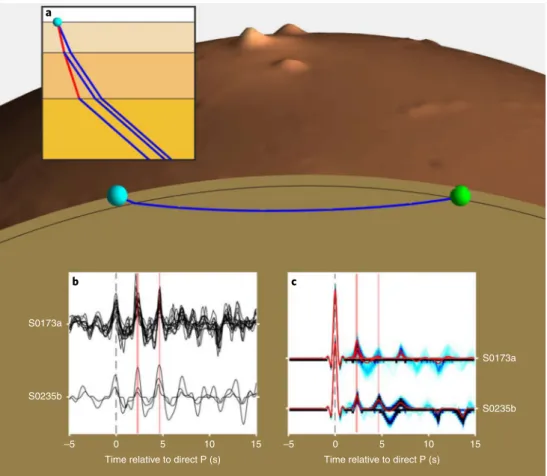
Fig. 6 | RF analysis for the Martian upper crust. A schematic background diagram showing the P-wave ray path from S0173 at 28° of epicentral distance4,27_{(green ball) to SEIS (light-blue ball). The ray path was obtained by raytracing with TTBox}48_{within an a priori Martian velocity model}39_. Topography is derived from MOLA data49_{and exaggerated vertically by a factor of 8. Mountains in the background are the Elysium Montes north of} InSight. a, Zoom-in on the crust below SEIS, illustrating crustal structure and the origin of the receiver-side converted phases analysed here. The incident plane P wave is indicated by blue rays, while the S waves resulting from P-to-S conversion at each of the two crustal discontinuities are shown in red. Raytracing is done in a velocity model consistent with the results of the RF inversion (Supplementary Discussion 4–4) and Supplementary Table 4–1, so that the two illustrated conversions correspond to the two peaks observed at 2.2–2.4 s and 4.6–4.7 s in the RFs. In addition, the ray for the direct P wave is shown. b, Various estimates of the P-to-S RFs for S0173a and S0235b, resulting from different deglitching and deconvolution methods as described in Supplementary Discussions 4 and 5. The main consistent positive arrivals as discussed in the text are marked in orange. c, RF estimates based on transdimensional hierarchical Bayesian deconvolution. The blue shading indicates the probability of a certain amplitude at a certain time, with darker shades corresponding to a higher probability. Probabilities for all four deglitching methods are combined for S0173a. Red lines indicate individual average RFs, and orange bars mark main arrivals as in b.

(8)

The converted phases can be extracted from seismograms by deconvolving the incoming P wavetrain on the vertical component from the radial component, which minimizes complexity due to source effects and propagation through Mars’s interior. Individual arrivals associated with subreceiver conversions can then be readily identified in the resulting P-to-S RF.

Over the past 40 years, RFs have become a standard method to

study crustal and upper-mantle structure of the Earth33,34_{and have}

also been applied to lunar seismic data35,36_{. See Supplementary}

Discussion 4 and Supplementary Figs. 4-2–4-4 for the specific methodology used.

We focus on the early part of P-to-S RFs (0–5 s) of S0173a and S0235b, which is related to crustal structure37_{. Both events have distinct}

seismic arrivals and their epicentres are ~450 km apart, at ~26°−28°

epicentral distance4_{. A broadband ‘glitch’ contaminates the VBB}

seismograms of S0173a about 15 s after the P onset (Supplementary Figs. 1–9), requiring glitch removal (Supplementary Discussion 5).

Figure 6b,c shows RFs obtained for several deglitching

algo-rithms and RF methods. See Supplementary Discussion 4 for details. The variability between individual results provides an esti-mate of the single-event RF uncertainty. An alternative estiesti-mate can be obtained by applying transdimensional hierarchical Bayesian

deconvolution38_{, which yields an ensemble of RFs compatible with}

the data (Fig. 6c). An initial positive arrival is consistently observed for all methods at 2.2–2.4 s, followed by a second positive arrival 4.6–4.7 s after the P wave. The later part of the RFs shows higher variability among different methods.

The same two phases are also observed in the RFs for the glitch-free S0235b event. These two quakes are located in

dif-ferent directions from InSight (91o_{back azimuth for S0173a}

ver-sus 74o_{for S0235b), which suggests that the phases are caused by}

crustal layering beneath the receiver rather than distributed scat-terers along their propagation paths. Clear multiple converted and reflected phases could not yet be unambiguously identified within these data. The peak at 2.2–2.4 s indicates a discontinuous veloc-ity increase between 8 and 11 km depth and an S-wave velocveloc-ity of

1.7–2.1 km s−1_{within the topmost layer (see Supplementary}

Discussion 4 and Supplementary Figs. 4–9). The nearly constant relative timing between the peaks at 2.2–2.4 and 4.6–4.7 s and a phase around 7 s observed in some of the different realizations of the RF could indicate that these phases are reverberations gener-ated at the same velocity contrast with comparable travel time for each additional reflection. However, the absence of any unambigu-ous accompanying negative arrivals and the comparatively large apparent P-wave incidence angles of more than 25° as derived from various polarization measurements (see Supplementary Figs. 4–8) argue against reverberations in a near-surface low-velocity layer (Supplementary Figs. 4–6 and 4–7) and are more compatible with structure at depth causing the later arrivals.

No signals before 2.2 s, including oscillating waveforms as expected for a shallow strong impedance contrast, are found. The regolith layer is therefore not resolved by the RFs and must be thin-ner than a few tens of metres (see Supplementary Discussion 4 and Supplementary Figs. 4–5), in agreement with our compliance anal-ysis. The transverse components of the RFs are at the noise level of the vertical components, thus we have no evidence for crustal anisotropy (Supplementary Figs. 4–5).

First seismic constraints on the Martian crust

Even though large quakes with multiple surface wave arrivals39–41

or located impacts42_{have not yet been detected, SEIS already}

con-strains the Martian crust and utilizes a new source of seismic infor-mation through the interaction of the Martian atmosphere with the ground.

SEIS data confirm, with both compliance and RFs, a thin (few metres) regolith layer over a more competent layer in the vicinity

of the lander. Much deeper, a crustal layer with S-wave velocity

between 1.7 and 2.1 km s−1_{extending down to 8 and 11 km depth is}

suggested by the first SEIS RF analysis. Gamma Ray Spectrometer

chemical mapping43_{and geology}44_{suggest that the uppermost}

crustal layers are composed of basaltic rocks. Velocities reduced by up to 50% with respect to Earth’s analogues (Supplementary

Table 4–1) imply therefore highly altered and/or damaged layers45_.

Finally, the attenuations inferred from S0128a, S0173a and S0235b are significantly higher than in the lunar crust,

suggest-ing a crust with small amounts of volatiles46_{. As the diffusivity}

and thickness of the crust remain weakly constrained, we cannot entirely reject the possibility that these attenuations reflect energy leakage. However, inversions of S0173a and S0235b data indicate that absorption may well be the dominant process and is

compa-rable to that of Earth’s crystalline massifs. The Qi from S0173a and

S0235b signals agrees with the lithospheric Qi proposed prelaunch45.

Further work will be needed to confirm this interpretation and to delineate more precisely the stratification of attenuation in the Mars crust and lithosphere.

Additional locatable events, especially at larger epicentral dis-tances, and complementary methods (for example, noise auto-correlations), will reduce uncertainties and will provide tighter constraints on the elastic and anelastic structure, including the depth of the crust/mantle discontinuity. Events with Mw > 4.5 will

ultimately provide the deep interior’s constraints5,39_.

References

1. Banerdt, B. et al. Initial results from the InSight mission on Mars. Nat. Geosci.

https://doi.org/10.1038/s41561-020-0544-y (2020).

2. Golombek, M. et al. Geology of the InSight landing site on Mars.

Nat. Commun. https://doi.org/10.1038/s41467-020-14679-1 (2020). 3. Anderson, D. L. et al. Seismology on Mars. J. Geophys. Res. 82,

4524–4546 (1977).

4. Giardini, D. et al. The seismicity of Mars. Nat. Geosci. https://doi.org/10.1038/ s41561-020-0539-8 (2020).

5. Lognonné, P. et al. SEIS: InSight’s Seismic Experiment for Internal Structure of Mars. Space Sci. Rev. 215, 12 (2019).

6. Banfield, D. et al. InSight Auxiliary Payload Sensor Suite (APSS). Space Sci.

Rev. 215, 4 (2019).

7. Banfield, D. et al. The atmosphere of Mars as observed by InSight.

Nat. Geosci. https://doi.org/10.1038/s41561-020-0534-0 (2020).

8. Trebi-Ollennu, A. et al. InSight Mars lander robotics instrument deployment system. Space Sci. Rev. 214, 93 (2018).

9. Maki, J. N. et al. The color cameras on the InSight lander. Space Sci. Rev. 214, 105 (2018).

10. Peterson J. Observations and Modelling of Background Seismic Noise Open-File Report 93-322 (US Geological Survey, 1993).

11. Lognonné, P. & Johnson, C. L. in Treatise on Geophysics 2nd edn, Vol. 10 (ed. Schubert, G.) 65–120 (Elsevier, 2015).

12. Spiga, A. et al. Atmospheric science with InSight. Space Sci. Rev. 214, 109 (2018).

13. Lognonné, P. & Mosser, B. Planetary seismology. Surv. Geophys. 14, 239–302 (1993).

14. Murdoch, N. et al. Evaluating the wind-induced mechanical noise on the InSight seismometers. Space Sci. Rev. 211, 429–455 (2017).

15. Kenda, B. et al. Modeling of ground deformation and shallow surface waves generated by Martian dust devils and perspectives for near-surface structure inversion. Space Sci. Rev. 211, 501–524 (2017).

16. Murdoch, N. et al. Estimations of the seismic pressure noise on Mars determined from Large Eddy Simulations and demonstration of pressure

(9)

decorrelation techniques for the InSight mission. Space Sci. Rev. 211, 457–483 (2017).

17. Murdoch, N. et al. Flexible mode modelling of the InSight lander and consequences for the SEIS instrument. Space Sci. Rev. 214, 117 (2019). 18. Mimoun, D. et al. The noise model of the SEIS seismometer of the InSight

mission to Mars. Space Sci. Rev. 211, 383–428 (2017).

19. Fayon, L. et al. A numerical model of the SEIS leveling system transfer matrix and resonances: application to SEIS rotational seismology and dynamic ground Interaction. Space Sci. Rev. 214, 119 (2018).

20. Spohn, T. et al. The heat flow and physical properties package (HP3_{) for the}

InSight mission. Space Sci. Rev. 214, 96 (2018).

21. Kedar, S. et al. Analysis of regolith properties using seismic signals generated by InSight’s HP3 penetrator. Space Sci. Rev. 211, 315 (2017).

22. Brinkman, N. et al. The first active seismic experiment on Mars to characterize the shallow subsurface structure at the InSight landing site.

SEG Tech. Prog. Expand. Abstr. 4756–4760 (2019).

23. Sorrells, G. G. A preliminary investigation into the relationship between long-period seismic noise and local fluctuations in the atmospheric pressure field. Geophys. J. Int. 26, 71–82 (1971).

24. Lorenz, R. D. et al. Seismometer detection of dust devil vortices by ground tilt. Bull. Seism. Soc. Am. 105, 3015–3023 (2015).

25. Morgan, P. et al. A pre-landing assessment of regolith properties at the InSight landing site. Space Sci. Rev. 214, 104 (2018).

26. Delage, P. et al. An investigation of the mechanical properties of some Martian regolith simulants with respect to the surface properties at the InSight mission landing site. Space Sci. Rev. 211, 191–213 (2017). 27. InSight Marsquake Service Mars Seismic Catalogue: InSight Mission V1

2/1/2020 (ETHZ, IPGP, JPL, ICL, ISAE-Supaero, MPS, Univ. Bristol, 2020). 28. Dainty, A. M. et al. Seismic scattering and shallow structure of the moon in

oceanus procellarum. Moon 9, 11–29 (1974).

29. Margerin, L., Campillo, M., Van Tiggelen, B. & Hennino, R. Energy partition of seismic coda waves in layered media: theory and application to Pinyon Flats observatory. Geophys. J. Int. 177, 571–585 (2009).

30. Margerin, L., Campillo, M., Shapiro, N. & van Tiggelen, B. A. Residence time of diffuse waves in the crust as a physical interpretation of coda Q: application to seismograms recorded in Mexico. Geophys. J. Int. 138, 343–352 (1999).

31. Romanowicz, B. A. & Mitchell, B. J. in Treatise on Geophysics 2nd edn, Vol. 1 (ed. Schubert, G.) 789–827 (Elsevier, 2015).

32. Gillet, K., Margerin, L., Calvet, M. & Monnereau, M. Scattering attenuation profile of the moon: implications for shallow moonquakes and the structure of the megaregolith. Phys. Earth Planet. Int. 262, 28–40 (2017).

33. Langston, C. A. Structure under Mount Rainier, Washington, inferred from teleseismic body waves. J. Geophys. Res. 84, 4749–4762 (1979).

34. Abt, D. L. et al. North American lithospheric discontinuity structure imaged by Ps and Sp receiver functions. J. Geophys. Res. 115, B09301 (2010). 35. Vinnik, L., Chenet, H., Gagnepain-Beyneix, J. & Lognonné, P. First seismic

receiver functions on the Moon. Geophys. Res. Lett. 28, 3031–3034 (2001). 36. Lognonné, P., Gagnepain-Beyneix, J. & Chenet, H. A new seismic model of

the Moon: implication in terms of structure, formation and evolution.

Earth Planet. Sci. Lett. 112, 27–44 (2003).

37. Knapmeyer-Endrun, B., Ceylan, S. & van Driel, M. Crustal S-wave velocity from apparent incidence angles: a case study in preparation of InSight. Space

Sci. Rev. 214, 83 (2018).

38. Kolb, J. & Lekic, V. Receiver function deconvolution using transdimensional hierarchical Bayesian inference. Geophys. J. Int. 197, 1719–1735 (2014). 39. Panning, M. P. et al. Planned products of the Mars Structure Service for the

InSight mission, Mars. Space Sci. Rev. 211, 611–650 (2017).

40. Panning, M. P. et al. Verifying single-station seismic approaches using Earth-based data: preparation for data return from the InSight mission to Mars. Icarus 248, 230–242 (2015).

41. Khan, A. M. et al. Single-station and single-event marsquake location and inversion for structure using synthetic Martian waveforms. Phys. Earth

Planet. Inter. 258, 28–42 (2016).

42. Daubar, I. et al. Impact-seismic investigations of the InSight mission.

Space Sci. Rev. 214, 132 (2018).

43. Baratoux, D., Toplis, M. J., Monnereau, M. & Gasnault, O. Thermal history of Mars inferred from orbital geochemistry of volcanic provinces. Nature 472, 338–341 (2011).

44. Golombek, M. et al. Selection of the InSight landing site. Space Sci. Rev. 211, 5–95 (2017).

45. Smrekar, S. E. et al. Pre-mission InSights on the interior of Mars. Space Sci.

Rev. 215, 3 (2019).

46. Tittmann, B. R., Clark, V. A., Richardson, J. M. & Spencer, T. W. Possible mechanism for seismic attenuation in rocks containing small amounts of volatiles. J. Geophys. Res. 85, 5199–5208 (1980).

47. Clinton, J. et al. The Marsquake Service: securing daily analysis of SEIS data and building the Martian seismicity catalogue for InSight. Space Sci. Rev. 214, 133 (2018).

48. Knapmeyer, M. TTBox: a MatLab toolbox for the computation of 1D teleseismic travel times. Seismol. Res. Lett. 75, 726–733 (2004). 49. Smith, D. E. et al. Mars Orbiter laser altimeter: experiment summary

after the first year of global mapping of Mars. J. Geophys. Res. 106, 23689–23722 (2001).

1_{Université de Paris, Institut de Physique du Globe de Paris, CNRS, Paris, France.}2_{Institut Universitaire de France, Paris, France.}3_{Jet Propulsion Laboratory,} California Institute of Technology, Pasadena, CA, USA. 4_{Department of Electrical and Electronic Engineering, Imperial College London, London, UK.} 5_{Institute of Geophysics, ETH Zurich, Zurich, Switzerland.}6_{Max Planck Institute for Solar System Research, Göttingen, Germany.}7_{Institut Supérieur de} l’Aéronautique et de l’Espace—SUPAERO, Toulouse, France. 8_{Bensberg Observatory, University of Cologne, Bergisch Gladbach, Germany.}9_{Institut de} Recherche en Astrophysique et Planétologie, Université Toulouse III Paul Sabatier, CNRS, CNES, Toulouse, France. 10_{Department of Earth and Planetary} Sciences, University of California Santa Cruz, Santa Cruz, CA, USA. 11_{Université de Lyon, Université Claude Bernard Lyon 1, ENS, CNRS, Laboratoire de} Géologie de Lyon—Terre, Planètes, Environnement, Villeurbanne, France. 12_{Sorbonne Université, Muséum National d’Histoire Naturelle, UMR CNRS 7590,} Institut de Minéralogie, de Physique des Matériaux et de Cosmochimie, IMPMC, Paris, France. 13_{Laboratoire de Planétologie et Géodynamique, UMR6112,} Université de Nantes, Université dAngers, CNRS, Nantes, France. 14_{Department of Earth, Planetary, and Space Sciences, University of California,} Los Angeles, CA, USA. 15_{Space Exploration Institute, Neuchâtel, Switzerland.}16_{Institute of Theoretical Physics, University of Zürich, Zürich, Switzerland.} 17_{DLR Institute of Planetary Research, Berlin, Germany.}18_{Department of Geology, University of Maryland, College Park, College Park, MD, USA.}19_Laboratoire de Météorologie Dynamique/Institut Pierre Simon Laplace (LMD/IPSL), Sorbonne Université, Centre National de la Recherche Scientifique (CNRS), École Polytechnique, École Normale Supérieure (ENS), Paris, France. 20_{Black Forest Observatory, Stuttgart University, Wolfach, Germany.}21_{Department of} Geophysics, Colorado School of Mines, Golden, USA. 22_{Ecole des Ponts ParisTech, Laboratoire Navier/CERMES, CNRS, Marne la Vallée, France.}23_{School of} Earth Sciences, University of Bristol, Bristol, UK. 24_{Department of Geosciences, Princeton University, Princeton, NJ, USA.}25_{Johns Hopkins Applied Physics} Laboratory, Laurel, MD, USA. 26_{Université de Lyon, École Normale Supérieure de Lyon, UCBL, CNRS, Laboratoire de Géologie de Lyon—Terre, Planètes,} Environnement, Lyon, France. 27_{Department of Earth Sciences, University of Oxford, Oxford, UK.}28_{Centre National d’Etudes Spatiales, Toulouse, France.} 29_{Institute of Earth Sciences Jaume Almera (ICTJA), Barcelona, Spain.}30_{International Space Science Institute, Bern, Switzerland.}31_{Division of Soil Mechanics} and Foundation Engineering, Technical University of Kaiserslautern, Kaiserslautern, Germany. 32_{NASA MSFC, NSSTC, Huntsville, AL, USA.}33_{Cornell Center} for Astrophysics and Planetary Science, Cornell University, Ithaca, NY, USA. 34_{Department of Physics, University of Oxford, Oxford, UK.}35_{Department of} Earth, Ocean and Atmospheric Sciences, University of British Columbia, Vancouver, BC, Canada. 36_{Planetary Science Institute, Tucson, AZ, USA.}37_{Centro de} Astrobiologia—Instituto Nacional de Tecnica Aeroespacial, Torrejón de Ardoz, Spain. 38_{Atmospheric, Oceanic and Planetary Physics, University of Oxford,} Oxford, UK. 39_{Université Côte d’Azur, Observatoire de la Côte d’Azur, Laboratoire Lagrange, CNRS, Nice, France. ✉e-mail:}_{lognonne@ipgp.fr}

(10)

Methods

Details of methods related to the SEIS raw data analysis are given in the Supplementary Information. This section describes in more detail the inversion method used in Supplementary Discussions 2 and 4 for shallow layer structure inversions.

Subsurface analysis and Supplementary Discussion 2. A Markov chain Monte

Carlo algorithm is used to sample solutions (that is, physical configurations) of the inverse problem that both fit the observations within errors and satisfy known (or assumed) physical a priori constraints. We employ a Bayesian probabilistic procedure developed50_{and tested for prelaunch works}39,40,42_.

Bayesian approaches51_{allow us to go beyond the classical computation of the}

unique best-fitting model by providing a quantitative probabilistic measure of the model resolution, uncertainties and non-unicity. One important advantage of this method is complete independence from the choice of the starting model. To estimate the posterior distribution of the parameters, we employ the Metropolis–Hastings algorithm52,53_{, which samples the model space with a}

sampling density proportional to the unknown posterior PDF. Using a large number of iterations, the samples provide a good approximation of the posterior distribution for the model parameters.

The algorithm used in the paper is divided into four steps.

(1) The model parameters (Young’s modulus and Poisson’s ratio) are randomly sampled in the parameter space. The model is divided into two parts: the regolith and the bedrock. The Young’s modulus and Poisson’s ratio at the surface are randomly sampled during the inversion. Equations 1 and 20 from ref. 25_are

then used to compute the whole Young’s modulus and Poisson’s ratio profile as a function of depth within the regolith layer. The depth of the regolith/bedrock interface is randomly sampled between the surface and 20 m. The bedrock is supposed to be made of one layer.

(2) Forward problem computation. The compliance as a function of frequency is calculated in the case of a horizontally layered half space23_{. The solution to the}

elastostatic equation is obtained with a Thomson–Haskell propagator method54_.

(3) Computation of the misfit, which determines the difference between the observed data and the computed synthetic data. The input compliance as a function of frequency data is provided in the form of a two-dimensional matrix, which gives a weight to each (frequency, compliance) couple. In practice, each time a new model is randomly sampled, a weight is given for each frequency according to the compliance value in the two-dimensional matrix. The sum of the weights for all the frequencies gives the misfit value.

(4) The current model is accepted or rejected, using the Metropolis–Hastings algorithm52,53_{. This algorithm relies on a randomized decision rule, which accepts}

or rejects the proposed model according to its fit to the data and the prior. (5) A new model is proposed by randomly perturbing the previously accepted model. Here, the sampling of the parameter space is performed using a Gaussian function centred on the last accepted value of the parameters.

RF analysis and Supplementary Discussion 4. Five different groups calculated

RFs to compare the results of different techniques, specifically of different deconvolution methods. One of the applied methods is probabilistic and produces an ensemble of RFs. For this method, upgoing P and SV waveforms were obtained from the Z and R waveforms by applying a free-surface transfer matrix55_{. As}

this matrix depends on the ray parameter as well as near-surface P- and S-wave velocities, these velocities were estimated by minimizing the energy of the SV component during the first 2 s of the P-wave arrival34_{. The deconvolution itself}

was performed by applying the transdimensional hierarchical Bayesian deconvolution method38_{. The method uses a reversible jump Markov chain}

Monte Carlo algorithm to sample one million random realizations of RFs, represented by Gaussian pulses of unknown width, lag time and amplitude. The number of these pulses in the RFs is also an unknown that is determined during the sampling process.

The other four groups worked with deterministic methods. To produce the RFs shown in Fig. 6, two groups applied iterative time-domain deconvolution56_{. The}

code for this method is available at http://eqseis.geosc.psu.edu/cammon/HTML/ RftnDocs/thecodes01.html. Details of parameters used are given in Supplementary Discussion 4. One group applied spectral whitening and cross-correlation57_{. The}

parameters used in the processing and comparison of results with other methods are detailed in Supplementary Discussion 4. The final group calculated RFs by using a time-domain Wiener filter that transforms the complex P wavetrain on the Z component into a band-limited spike58,59_{. This Wiener filter was applied to}

all three components of the seismogram to produce the RFs. The processing was implemented in Seismic Handler (http://www.seismic-handler.org/) by using the

spiking and fold commands. Results are compared for different parameter settings

in Supplementary Discussion 4.

Inversion of RFs and apparent S-wave velocities (Supplementary Figs. 4–9) was performed using the Neighbourhood Algorithm as implemented in dinver60

(www.geopsy.org). The forward computation of the RF waveforms in the inversion as well as those shown in Supplementary Figs. 4–6 uses the FORTRAN code by Shibutani et al.61_{contained in the original Neighbourhood Algorithm}

implementation by Sambridge62₍_{http://www.iearth.org.au/codes/NA/}_).

Data availability

All InSight SEIS data63_{used in this paper are available from the IPGP Data Center,}

IRIS-DMC and NASA PDS; all InSight APSS data are available from NASA PDS (https://pds-geosciences.wustl.edu/missions/insight/index.htm). The data used for Fig. 2 have been obtained from IRIS/DMC for Black Forest Observatory64_{and from}

IPGP Data Center for lunar data (Code XA, http://datacenter.ipgp.fr/data.php). The data displayed in Fig. 5 correspond to the following events. A is a broadband (1–10-Hz) shallow Moonquake waveform recorded on 13 March 1973, at Apollo Station 15; the inferred hypocentre is latitude −84°, longitude −134° (ref. 65_{). B are}

S0128 and S0173 events described in the main text. C is a broadband (1–10-Hz) regional crustal earthquake waveform recorded on 28 April 2016, at the broadband station ATE (https://doi.org/10.15778/RESIF.FR); the hypocentre is latitude 46.04°, longitude −1.04°, depth 15 km (BCSF bulletin, http://renass.unistra.fr).

D is a broadband (1–10-Hz) waveform recorded on 22 February 2000, at Mount St. Helens station ESD66_{(now EDM); the hypocentre is latitude 46.1472°, longitude}

−122.1457°, depth = 10.4 km (event 10495398, PNSN bulletin, https://pnsn.org). P and S arrival times for S0128a, S0173a and S0235b are from the MQS47

catalogue27_{. The S–P travel-time difference used in the scattering analysis is 75 s,}

compatible with the reported27_{value of 84 ± 28 s. Subsets for the models proposed}

for the subsurface and a summary for the upper crust are available (Supplementary Tables 1 and 2 for subsurface, Supplementary Table 3 for upper crust). See Supplementary Discussions 2 and 4 respectively for more details.

Code availability

See Methods for publicly available codes and for associated algorithms. The multiple-scattering simulation codes used in Supplementary Discussion 3 are available on request from L.M. (ludovic.margerin@irap.omp.eu).

References

50. Drilleau, M. et al. A Bayesian approach to infer radial models of temperature and anisotropy in the transition zone from surface wave dispersion curves.

Geophys. J. Int. 195, 1165–1183 (2013).

51. Mosegaard, K. & Tarantola, A. Monte Carlo sampling of solutions to inverse problems. J. Geophys. Res. 1001, 12431–12448 (1995).

52. Metropolis, N., Rosenbluth, A. W., Rosenbluth, M. N., Teller, A. H. & Teller, E. Equation of state calculations by fast computing machines.

J. Chem. Phys. 21, 1087–1091 (1953).

53. Hastings, W. K. Monte Carlo sampling methods using Markov chains and their applications. Biometrika 57, 97–109 (1970).

54. Sorrells, G. G., McDonald, J. A., Der, Z. A. & Herrin, E. Earth motion caused by local atmospheric pressure changes. Geophys. J. Int. 26, 83–98 (1971). 55. Kennett, B. L. N. The removal of free surface interactions from

three-component seismograms. Geophys. J. Int. 104, 53–163 (1991).

56. Ligorria, J. P. & Ammon, C. J. Iterative deconvolution and receiver-function estimation. Bull. Seism. Soc. Am. 89, 1395–1400 (1999).

57. Tauzin, B., Phạm, T. S. & Tkalčić, H. Receiver functions from seismic interferometry: a practical guide. Geophys. J. Int. 217, 1–24 (2019). 58. Kind, R., Kosarev, G. L. & Petersen, N. V. Receiver functions at the stations

of the German Regional Seismic Network (GRSN). Geophys. J. Int. 121, 191–202 (1995).

59. Hannemann, K., Krüger, F., Dahm, T. & Lange, D. Structure of the oceanic lithosphere and upper mantle north of the Gloria Fault in the eastern mid-Atlantic by receiver function analysis. J. Geophys. Res. 122, 7927–7950 (2017).

60. Wathelet, M. An improved Neighborhood Algorithm: parameter conditions and dynamic scaling. Geophys. Res. Lett. 35, L09301 (2008).

61. Shibutani, T., Sambridge, M. & Kennett, B. Genetic algorithm inversion for receiver functions with application to crust and uppermost mantle structure beneath eastern Australia. Geophys. Res. Lett. 23, 1829–1832 (1996). 62. Sambridge, M. Geophysical inversion with a neighbourhood algorithm—I.

Searching a parameter space. Geophys. J. Int. 138, 479–494 (1999). 63. SEIS Raw Data: InSight Mission (InSight Mars SEIS Data Service, IPGP, JPL,

CNES, ETHZ, ICL, MPS, ISAE-Supaero, LPG, MSFC, 2019); https://doi. org/10.18715/SEIS.INSIGHT.XB_2016

64. Black Forest Observatory Data (GFZ Data Services, Black Forest Observatory, 1971); https://doi.org/10.5880/BFO

65. Nakamura, Y. et al. Shallow moonquakes: Depth, distribution and implications as to the present state of the lunar interior. In Proc. Lunar Sci.

Conf. 10th Vol. 3, 2299–2309 (Pergamon Press, 1979).

66. Pacific Northwest Seismic Network (International Federation of Digital Seismograph Networks, Univ. Washington, 1963). https://doi. org/10.7914/SN/UW

Acknowledgements

We acknowledge NASA, CNES, their partner agencies and institutions (UKSA, SSO, DLR, JPL, IPGP-CNRS, ETHZ, IC, MPS-MPG) and the flight operations team at JPL, SISMOC, MSDS, IRIS-DMC and PDS for providing SEED SEIS data. The French team acknowledge the French Space Agency CNES, which has supported and funded all

(11)

SEIS-related contracts and CNES employees, as well as CNRS and the French team universities for personal and infrastructure support. SEIS VBB testing and development have also been supported by SESAME (Ile de France, Université Paris Diderot, IPGP, CNES) in the frameworks Centre de simulation Martien I-07–603 and Pole Terre Planètes 11015893. Additional support was provided by ANR (ANR-14-CE36-0012-02, ANR-19-CE31-0008-08 for SEIS science support and ANR-11-EQPX-0040 for RESIF data access) and for the IPGP team by the UnivEarthS Labex program (ANR-10-LABX-0023) and IDEX Sorbonne Paris Cité (ANR-11-IDEX-0005-0). Regolith stratigraphy inversion used HPC resources of CINES under allocation A0050407341 attributed by GENCI (Grand Equipement National de Calcul Intensif). Research described in this paper was partially carried out by the InSight Project, Jet Propulsion Laboratory, California Institute of Technology, under a contract with NASA. Additional work was supported by NASA’s InSight Participating Scientist Program and LPI (LPI is operated by USRA under a cooperative agreement with the Science Mission Directorate of the NASA). The Swiss coauthors were jointly funded by (1) the Swiss National Science Foundation and French Agence Nationale de la Recherche (SNF-ANR project 15713, Seismology on Mars), (2) the Swiss State Secretariat for Education, Research and Innovation (SEFRI project MarsQuake Service—Preparatory Phase) and (3) ETH Research grant ETH-06 17-02. Additional support came from the Swiss National Supercomputing Centre (CSCS) under project s992. The Swiss contribution in implementation of the SEIS electronics was made possible through funding from the federal Swiss Space Office (SSO), the contractual and technical support of the ESA-PRODEX office. SEIS-SP development and delivery were funded by UKSA. The SEIS levelling system development and operation support at MPS was funded by the DLR German Space Agency. B.T. and L. Pan acknowledge funding from European Union’s Horizon 2020 research and innovation programme under Marie Sklodowska-Curie grant agreements 793824 and 751164. This paper is InSight Contribution 101, LPI contribution 2249 and IPGP Contribution 4099.

Author contributions

P. Lognonné leads the SEIS experiment and the VBB sensors. He designed the higher-level requirements of the experiment together with D. Mimoun. He led the manuscript team effort, contributed to several Supplementary Discussions and integrated all contributions. W.B.B. leads the InSight mission and the US contribution to SEIS. W.T.P., D.G. and U.C. lead the SP, Ebox and LVL respectively. W.T.P. contributed to several Supplementary Discussions. D.B., J.M. and C.T.R. lead the APSS, TWINS and IFG instruments. E. Barrett contributes to the SEIS operation at JPL, together with C.Y. at CNES. M. Bierwirth for the LVL, S. Calcutt for the SP, D. Mance and P.Z. for the Ebox, K.H. for the tether-shielding and S. de R., T.N., O.R. and S. Tillier for the VBB contributed to the SEIS subsystems and the SEIS Mars deployment and commissioning. L.K., G.P., P. Laudet and A.S.-B. contributed to the SEIS overall management and SEIS Mars deployment and commissioning. J.C., M. Böse, C.C., S. Ceylan, M. van D., A.H., A.K., T.K., G.M., J.-R.S. and S. Stähler contribute to the MQS frontline activity, and D.G., W.B.B., P. Lognonné, D.B., R.F.G., D.G., S.K., M.P., W.T.P., S. Smrekar, A. Spiga and R.W. to the MQS review. E. Beucler, F.E., C.P. and S. Stähler contribute to the MQS and ERP operations. N.C. and C.J. contributed to the SEIS analysis and Mars deployment. C.B., E. Bozdag, I.D., M. Golombek, J.I., A.-C.P., R.L. and J.T. reviewed the manuscript. All authors read and commented on the manuscript. W.T.P. and P. Lognonné led the analysis of Supplementary Discussion 1. C.C., R.F.G., A. Stott, J.McC., C.P., S.B. and L. Pou analysed the data. D. Mimoun provided the environmental noise model. S. Ceylan provided the seismic event catalogue data. E.S. and M.S. provided the polarization analysis. L. Pou provided the VBB-POS output analysis. A. Spiga and D.B. provided the environmental data. P. Lognonné and S. Kedar led the analysis of Supplementary Discussion 2. L.F. developed the LVL inversion methodology with the support of

P. Lognonné. P. Delage and P. Lognonné discussed the results and P. Delage provided additional laboratory experiment support. L.F. and M. van D. performed the resonances analysis. T.S. leads the HP3_{experiment and contributed to the execution of the HP}3_-SEIS

experiment and the interpretation of the results. D.S. and F.A. implemented in collaboration with C.S. and J.R. the aliased-data reconstruction algorithm developed by D.S., F.A. and J.R. N.B., J. ten P. and C.S. implemented the clock time processing in collaboration with D.S. N.B., C.S., D.S. and M. van D. processed and interpreted the travel-time data in collaboration with J.R. C.S. and M. van D. contributed to the writing of the main text section related to the subsurface, and N.B., D.S., C.S. and M. van D. in collaboration with J.R. and F.A. wrote Supplementary Discussion 2. A.H. contributed to the HP3_{-SEIS analysis. S. Krasner, J.K., C.K., L.R., J.V. and N.V. developed the timing}

tools between the lander, HP3_{and SEIS. B.K. and N.M. developed the modelling}

and inversion tools for dust devils, processed the corresponding data and wrote Supplementary Discussion 2-3. C.P. and S.R. developed the automatic HiRise dust devil track software. M.D. developed the subsurface inversion tool with contributions from B.K. and P. Lognonné and wrote Supplementary Discussion 2-4. All authors discussed the overall results. N.T. and C.V. contributed to the discussion on regolith and duricrust properties. Supplementary Discussion 3 was written and led by L.M., T.K. and N.S. The scattering and attenuation scenarios for the sol 128 and sol 173 events were developed by T.K., P. Lognonné and L.M. R.F.G. provided deglitched waveforms. E.S., M.S. and E. Beucler analysed the polarization and incidence angle of the sol 173 event. Diffusion calculations were performed by W.T.P., N.S., L.M., P. Lognonné and M.P. Radiative transfer models were developed by L.M. M.C. and S.M. compiled the measurements and waveforms pertaining to Supplementary Fig. 3-12. The results were interpreted by P. Lognonné, T.K. and L.M. Reviews were provided by C.B., T.N.-M., A.-C.P. and R.W. B.K.-E., B.T. and M.P. coordinated the RF study in Supplementary Discussion 4. B.K.-E. (Method D), V.L. (Method A), B.T. (Method B), S. Tharimena (Method C) and A.K. and F.B. (Method E) calculated RFs using various methods, discussed the results, contributed to the interpretation, and drafted the manuscript. R.J. performed the inversion of S0173a data. B.K.-E. and B.T. calculated synthetic RFs. M.P. contributed to the interpretation and participated in discussions and writing. P. Davis, P. Lognonné, B.P., R.F.G. and J.-R.S. contributed deglitched waveforms for S0173a. S. Stähler provided the probability distribution of ray parameters for S0173a. M.K. produced the schematic diagrams in Fig. 6 and participated in discussions. The elastic property compilation was provided by C.P., L. Pan, D.A., A.J., C.M., M. Golombek, A.K., N.F. and C.Q.-N. C.B. and J.I. reviewed this supplementary material. J.-R.S. coordinated Supplementary Discussion 5 with P. Davis and R.W.-S. F.N. and P. Lognonné led the glitch-focused working group. P. Davis, P. Lognonné, L. Pou, B.P. and R.F.G. developed the glitch-removal algorithm based on the instrument transfer function. S.B., P. Lognonné and E.S. developed the removal algorithm based on the deep scattering tool. J.-R.S. developed the glitch-removal algorithm based on the discrete wavelet transform. All authors analysed the glitches, discussed the removal strategies and approved of the manuscript.

Competing interests

The authors declare no competing interests.

Additional information

Supplementary information is available for this paper at https://doi.org/10.1038/

s41561-020-0536-y.

Correspondence and requests for materials should be addressed to P.L. Peer review information Primary Handling Editor: Stefan Lachowycz.

Reprints and permissions information is available at www.nature.com/reprints.