O
pen
A
rchive
T
OULOUSE
A
rchive
O
uverte (
OATAO
)
OATAO is an open access repository that collects the work of Toulouse researchers and
makes it freely available over the web where possible.
This is an author-deposited version published in :
http://oatao.univ-toulouse.fr/
Eprints ID : 18139
To link to this article :
DOI: 10.4271/2015-01-2555.
URL :
http://dx.doi.org/10.4271/2015-01-2555.
To cite this version :
Suhir, Ephraim and Bensoussan, Alain and Nicolics,
Johann Predicted device-degradation failure-rate. (2015) In: SAE 2015
(SAE AeroTech Congress & Exhibition), 22 September 2015 - 24
September 2015 (Seattle, United States).
Any correspondence concerning this service should be sent to the repository
administrator:
[email protected]
Abstract
There is a concern that the continuing trend on miniaturization (Moore's law) in IC design and fabrication might have a negative impact on the device reliability. To understand and to possibly quantify the physics underlying this concern and phenomenon, it is natural to proceed from the experimental bathtub curve (BTC) - !"#$%&$#$'()*+%,,+-!'.)-/)'0")1"2$3"4)50$,)36!2")!"7"3',)'0")3-8&$9"1) effect of two major irreversible governing processes: statistics-related mass-production process that results in a decreasing failure rate with time, and reliability-physics-related degradation (aging) process that leads to an increasing failure rate. It is the latter process that is of major concern of a device designer and manufacturer.
The statistical process can be evaluated theoretically, using a rather simple predictive model. Owing to that and assuming that the two processes of interest are statistically independent one can assess the failure rates associated with the aging process from the BTC data by simply subtracting the predicted ordinates of the statistical failure rates (SFR) from the BTC ordinates. The objective of this analysis is to show how this could be done.
The suggested methodology proceeds from the concepts that the actual (“instantaneous”) SFR is a random variable with a known (assumed, established) probability distribution, that the experimental BTC can be represented by its infant mortality and the wear-out portions only (the steady-state portion in this case is simply the boundary between the infant mortality and wear-out portions) and that the two BTC portions considered can be approximated analytically. The cases, when the “instantaneous” SFR is distributed normally and in accordance with the Rayleigh law are used as suitable illustrations of the general concept.
The developed methodology can be employed when there is a need to better understand the relative roles of the statistics-related and physics-of-failure-related processes in reliability evaluations of electronic products. The methodology can be used also beyond the :"#1)-/);<)"9=$9""!$9=>)?0"9)'0"!")$,)%)9""1)'-)691"!,'%91)%91>) hence, to separate the roles of the two irreversible processes in question.
One of the major challenges of the future work is to determine the probability distributions of the actual (“instantaneous”) SFRs for particular products and applications.
Introduction
There is an indication [1] that the continuing trend on miniaturization (Moor's law) might have a negative impact on the device reliability. This trend is of particular concern when it comes to deep submicron (DSM) technologies characterized by etching thicknesses below 90nm and when device is operated at the wear out portion of the BTC, when the degradation (aging) process plays the major role. To better understand and possibly quantify the reliability physics underlying DSM technologies, it is natural to proceed from the BTC - an experimental reliability “passport” of a population of mass +!-163"1)1"2$3",4)50")@5<)3-9,$1"!,)%91)!"7"3',>)0-?"2"!>)'0") combined effect of two governing irreversible processes: the statistics-related mass-production process and the reliability-physics-!"#%'"1)1"=!%1%'$-9)A%=$9=B)+!-3",,4)50"):!,')+!-3",,)!",6#',)$9)%) decreasing effective failure rate with time, while the second process leads to an increased failure rate. It is the latter process that is of major concern of the device manufacturer, and therefore there is an obvious need for being able to “extract” the degradation related /%$#6!")!%'")/!-8)'0")'-'%#)A-&,"!2"1B)/%$#6!")!%'")!"7"3'"1)&()'0") BTC.
Predicted Device-Degradation Failure-Rate
Ephraim Suhir
Portland State University
Alain Bensoussan
Institut de Recherche SAINT EXUPERY
Johann Nicolics
The statistical process can be assessed theoretically, using a simple predictive model [2]. Then, assuming that the two processes of interest are statistically independent, one can predict the failure rates associated with the degradation process by simply subtracting the SFR ordinates from the BTC data. The developed methodology shows how this could be done. It proceeds from an assumption that the actual (“instantaneous”) SFR is a random variable with a known (assumed or established) probability distribution. Normal and Rayleigh distributions of the random SFR are considered in this analysis as suitable illustrations of the general concept. The analytical representation of the BTC and the developed methodology can be employed in the design and analysis of the next generations of electron devices. It can be used also beyond the "#"3'!-9)1"2$3"):"#1>)?0"9)'0"!")$,)%)9""1)'-)%,,",,>)$9)2%!$-6,) engineering and applied science problems, the roles of the two governing irreversible processes in question.
Analysis
Analytical Bathtub Curve (BTC)
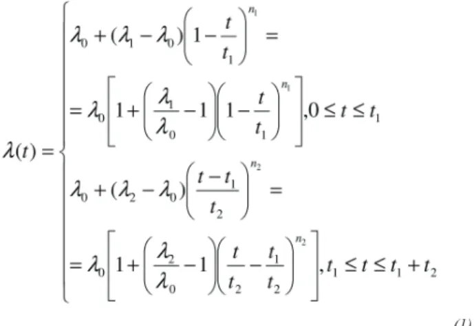
The experimental BTC (Fig.1) for the time dependent failure rate !(t) can be approximated as follows:
(1)
Here !0 is the minimum (“steady-state”) value of the BTC, !1 is the initial value of the failure rate (at the beginning of the infant mortality portion), t1 is the duration of this portion, !2)$,)'0"):9%#)2%#6")-/)'0") failure rate (at the end of the wear-out portion), t2 is the duration of this portion, and the exponents n1 and n2 are expressed through the fullnesses "1 and "2 of the infant -mortality and the wear-out BTC portions as 4)50",")/6##9",,",)%!")1":9"1)%,)'0")
ratios of the areas above the BTC to the areas (!1 - !0)t1 and (!2 - !0)t2 of the corresponding rectangulars. The exponents n1 and n2 change /!-8)C)'-)$9:9$'(>)?0"9)'0")/6##9",,",)"1 and "2 change from 0.5 (triangle) to 1 (rectangular). The lowest !(t) values can be achieved in the case of the largest "1 and "2 (or n1 and n2) values.
50"):!,')/-!86#%)$9)(1) describes the infant mortality portion of the BTC. The second formula is related to its wear-out portion. Both portions change slowly in the vicinity of their boundary. These slow changing regions of the BTC could be perceived and interpreted as the steady-state segment of the BTC. It is noteworthy that the analytical BTC in Fig.1 could be used for different applications, and should not be necessarily viewed as an 100% experimental information.
An experimental BTC [3] obtained during failure oriented accelerated '",'$9=)ADEF5B)-/)7$+G30$+),-#1"!)H-$9')$9'"!3-99"3'$-9,)$9)@"##)I%&,) Si-on-Si technology is shown in Fig.2, where the number of cycles is used instead of time. The data for the failure rates in the second line of Table 1 are obtained with the input information of "1 = 0.8 (n1 = 4),
"2 = 0.75 (n2 = 3), t1 = N1 = 75, t2 = N2 = 300, !0 = 0.5x10JK, ! 1 =
7.5x10JK, !
2 = 17.5x10JK. The probabilities PNF of non-failure are
shown in the third line of Table 1 assuming that the exponential law
PNF = e#!$ is applicable for the entire duration of testing. The
calculated data indicate that the time-dependence of the failure rate has a strong effect on the probability of non-failure.
Figure 1. Bathtub curve
Table 1. Failure rate and the probability of non-failure vs. number of cycles (see Fig.2)
Effective SFR of Mass-Produced Devices
A customer that receives products from n vendors can evaluate the probability of non-failure for the received products, assuming that the exponential law of reliability is applicable, as
(2)
Figure 2. Experimental BTC obtained for solder joint interconnections in L$G-9GL$)/#$+G30$+)86#'$G30$+)8-16#")@"##GI%&,)1",$=9
Here pk is the fraction of the products received from the k - th vendor,
!k is the (random) failure rate of these products, and t is time. Assuming that the actual (“instantaneous”) random failure rate can &">)$9)"//"3'>)%9()968&"!)&"'?""9)M"!-)%91)$9:9$'(>)'0"),68)$9)'0") formula (2) can be substituted, for a large n number, by the integral:
(3)
Here F(!) is the probability distribution function and f(!) is the probability density distribution function of the random failure rate !. The rationale behind the formulas (2) and (3) is as follows. The probability of non-failure of a large population of devices is determined by the failure rate of each particular device. The failure rate
(4)
changes in a random fashion from one device to another and is 1":9"1)%,)'0")!%'$-)-/)'0")36!!"9')!%'") of the number Nf (t) of devices that failed by the time t to the number Ns(t) of devices that remained sound by that time. Substituting, in accordance with the ergodic theorem, the number of the sound items with the probability
P(t) of their non-failure and the number of the failed items - with the
probability Q(t) = 1 - P(t) of failure one could write the formula (4) as
(5)
Considering (3), this formula can be written in the form:
(6)
<-8+6'%'$-9,)&%,"1)-9)'0$,)/-!86#%)3-9:!8)'0%')'0")"//"3'$2")LDN) decreases with time. In an extreme case, when the failure rate !(t) is distributed uniformly, the formula (6) yields: . This result leads to a very sharp decrease in the effective SFR with time and is viewed as a non-realistic.
Normally Distributed “Instantaneous” SFR
To assess the decrease in this rate with time for a more realistic distribution, let us assume that the SFR is normally distributed:(7)
Here is the mean value of the random failure rate ! and D is its variance. The effective SFR !ST (t) can be found as a function of time from the formula (6) and the distribution (7):
(8)
Here
(9)
(10)
and so are the auxiliary function
(11)
%91)'0")+!-&%&$#$'()$9'"=!%#)AI%+#%3")/693'$-9B
(12)
The function Erfc(xB)O)CJPAx) is sometimes referred to as
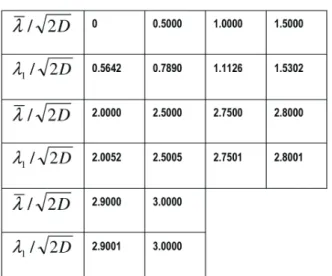
Weierstrass' zeta-function. The asymptotic expansion of the function can be used for large %N values, exceeding, say, 2.5. This expansion has been used when calculating the Table 2 data. The formula (10) indicates that the “physical” (effective) time depends not only on the actual time t, but also on the mean and variance of the accepted (established) distribution of the statistical failure rate. The function &N(%N) is tabulated in Table 2. This function changes from $9:9$'()'-)M"!->)?0"9)'0")1$8"9,$-9#",,)'$8")%N)30%9=",)/!-8)GQ)'-) Q4)D-!)1$8"9,$-9#",,)'$8",)&"#-?)JR4S)'0")/693'$-9) is ,$=9$:3%9'>),-)'0%')'0"),"3-91)'"!8)$9)(9) becomes small compared ?$'0)'0"):!,')'"!8>)%91)'0")/693'$-9)&N(%N) can be put equal to the dimensionless time %N itself, with an opposite sign though. At the initial moment of time (t = 0) the formulas (10), (11) and (8) yield:
(13)
With the initial value !ST'('!1 (the degradation failure rate !DG is obviously zero at the initial moment of time), the third formula in (13) yields:
(14)
When the ratio )30%9=",)/!-8)M"!-)'-)$9:9$'(>)'0")!%'$-)
changes from )'-)$9:9$'(4)50")!"#%'$-9,0$+)
(14) is tabulated in Table 3.
Table 3. The initial SFR vs. its mean value
As evident from the computed data, the initial failure rate can be put equal to its mean value, if the ratio exceeds 2.5. This is usually the case indeed, since the accepted normal distribution, when applied to a random variable that cannot be negative, should be 30%!%3'"!$M"1)&()%),$=9$:3%9')!%'$-)-/)$',)8"%9)2%#6")'-)'0"),'%91%!1) deviation, so that the negative values of the assumed distribution, although exist, are meaningless, i.e., do not contribute appreciably to the predicted information.
The statistics-related and physics-of-failure-related modes and mechanisms of failure take place concurrently. Assuming that the two irreversible processes in question are statistically independent, the total probability of non-failure at the given moment of time can be determined as a product of the statistics-related and reliability-physics-related probabilities of non-failure:
(15)
The calculated probabilities P(t) are shown, for the carried out numerical example, in the tenth line of Table 4. At the wear-out portion of the BTC they are obviously dominated by the low non-failure probabilities of the degradation process. The numerical example is carried out for the following input data: mean value (initial value) factor of the random failure rate:
; standard deviation of the failure rate:
; the initial failure rate: !1 = 8.4853x10JK1/hr;
the lowest failure rate: !0 = 9.6000x10JK1/hr; the highest (allowable)
failure rate: !2 = 19.8x10JK1/hr; duration of the infant mortality
portion: t1 = 48hr (burn-in time); duration of the wear out portion t2
= 39,952hr (obtained as the difference between the total time of
operation of 40,000hrs and the duration of the infant mortality portion); “fullnesses” of the infant mortality portion: "1 = 0.8 (n1 = 4); and the wear out portion:. "2 = 0.75 (n2 = 3). Calculations are performed in Table 4 and the probabilities of non-failure associated with the degradation process are shown in Table 5. The degradation related failure rates are computed, for each particular moment of time, as the difference between the ordinates of the experimentally obtained BTC (line 5 in Table 4) and the calculated (predicted) SFR (line 4 in Table 4). It is assumed that the infant mortality portion is short, so that no degradation takes place during this time, regardless of whether a burn-in effort is applied or not.
Table 5. Calculated probabilities-of-non-failure caused by the degradation process
For short times at the beginning of the infant mortality (burn-in) process, the function )$,),$=9$:3%9'>)%91)'0"),"3-91)'"!8)$9)'0") formula (9))$,),8%##)3-8+%!"1)'-)'0"):!,')'"!8>)%91)'0")#$9"%!)/-!86#%)
!ST = !1 - Dt)3%9)&")6,"1)'-)"2%#6%'")'0")LDN4);91""1>)'0$,),$8+#$:"1) formula predicts the SFR at the end of the infant mortality time as !ST = 84.834x10JShrJC. The exact number !
ST = 84.668x10
JShrJC is only
0.2% lower.
The obtained data indicate that the statistical probability of non-/%$#6!")1"3!"%,",)?$'0)'$8")%')'0")!%'0"!),$=9$:3%9')+-!'$-9)-/)'$8") despite the decrease in the SFR. At some moment of time (beginning with about 10,000 hours in the Table 4 example), the effect of the decreasing SFR starts to prevail, and the statistical probability of non-failure begins to increase with time. This circumstance does not play, however, an important role, because the degradation failure !%'",)&"3-8"),$=9$:3%9')%91),6++!",,)'0"),#$=0')$93!"%,")$9)'0") probability of non-failure associated with the SFR. In the line 8 of Table 4 the decrease in the probabilities of non-failure are shown assuming that the SFR remained at the initial level. The difference is large, especially for long times of operation, so that the change in the SFR with time should always be accounted for.
SFR Distributed According to Rayleigh Law
Assume now that the “instantaneous” failure rate is distributed in accordance with Rayleigh law, so that its probability distribution density function is
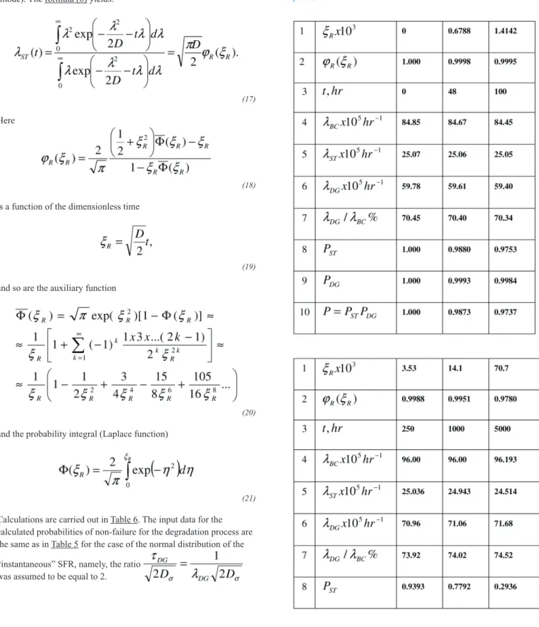
The standard deviation in this distribution is also its maximum value (mode). The formula (6) yields:
(17)
Here
(18)
is a function of the dimensionless time
(19)
and so are the auxiliary function
(20)
%91)'0")+!-&%&$#$'()$9'"=!%#)AI%+#%3")/693'$-9B
(21)
Calculations are carried out in Table 6. The input data for the calculated probabilities of non-failure for the degradation process are the same as in Table 5 for the case of the normal distribution of the “instantaneous” SFR, namely, the ratio
was assumed to be equal to 2.
Table 6. Calculated probabilities-of-non-failure caused by the degradation process
As one could see, the predicted data is rather different in the cases of the normal and Rayleigh distributions, and therefore the future work should include the analyses of the most suitable actual
(“instantaneous”) SFR distributions.
Summary/Conclusions
• Easy-to-use and physically meaningful predictive model that can be used in application to both die and packaging technologies has been developed for the assessment of the level of the time-dependent material degradation (aging) process from the available experimental BTC.
• Normal distribution of the actual (“instantaneous”) SFR results in substantially lower resulting probabilities of non-failure than Rayleigh law.
• Future work should include the assessment of the actual distributions of the “instantaneous” random failure rates of the statistical process for various electronic products and applications.
References
1. Regis, D., Berthon, J., and Gatti, M., “DSM Reliability Concerns - Impact on Safety Assessment,” SAE Technical Paper 2014-01-2197, 2014, doi:10.4271/2014-01-2197.
2. Suhir E., “Statistics- and Reliability-Physics-Related Failure T!-3",,",.>)U-1"!9)T0(,$3,)I"''"!,)@)AUTI@B>)V-#4)RW>)X-4)CY>) 2014
3. Suhir E., “Mechanical Reliability of Flip-Chip Interconnections in Silicon-on-Silicon Multichip Modules”, IEEE Conference on Multichip Modules, IEEE, Santa Cruz, Calif., March 1993.
Contact Information
Ephraim Suhir is at