Thinking outside the brackets : an alternative to the personal income tax brackets

(1)

THINKING OUTSIDE THE BRACKETS: AN ALTERNATIVE TO THE PERSONAL INCOME TAX BRACKETS Jean-François FRENETTE

INRS

Urbanisation, Culture et Société

JANUARY 2008

(2)

(3)

Thinking Outside the Brackets:

An Alternative to the Personal Income Tax

Brackets

Jean-François FRENETTE

Laboratoire d’analyse spatiale et d’économie régionale (LASER)

Institut national de la recherche scientifique Urbanisation, Culture et Société

(4)

Jean-François Frenette

jean-francois.frenette@ucs.inrs.ca

Inédits, collection dirigée par Mario Polèse

mario.polese@ucs.inrs.ca

Institut national de la recherche scientifique Urbanisation, Culture et Société

385, rue Sherbrooke

Montréal (Québec) H2X 1E3 Téléphone : (514) 499-4000 Télécopieur : (514) 499-4065 www.ucs.inrs.ca

(5)

Le degré de progressivité de la structure actuelle du régime d’impôt sur le revenu des particuliers au Canada est le produit d’une série de taux marginaux d’impositions et de tranches de revenu en combinaison avec un « montant personnel de base ». Ce modèle de base a été employé de façon ininterrompue depuis ses origines au début du 20e siècle; seulement les taux marginaux d’impositions et les tranches de revenu ont été modifiés au cours de cette période. Avec l’avènement des nouveaux services électroniques du gouvernement fédéral tel qu’IMPÔTNET, le besoin des « tranches d’impôts » dans le calcul de l’impôt prélevé du revenu imposable pourrait se voir devenir obsolète. L’objectif de cet article est d’explorer deux modèles pour calculer l’impôt sur le revenu à payer au Canada en employant une simple fonction quadratique ou logarithmique afin de définir les taux d’imposition marginaux et moyens comme alternatifs au système actuel de « tranches d’impôts ».

Mots-clés : Impôt sur le revenu des particuliers, Tranches d’impôt, Quadratique,

Logarithmique, Fonctions, Canada

The progressiveness of the current federal personal income tax structure in Canada is based on a series of marginal tax rates and income brackets combined with a “basic personal amount”. This standard model has been used uninterruptedly since its origins in the early 20th century; only the marginal tax rates and income brackets have been altered over time. With the advent of new federal government e-Services such as NETFILE, the need for “tax brackets” in calculating personal income tax payable could be rendered obsolete. The aim of this paper is to explore two models for calculating federal personal income tax payable in Canada using a simple quadratic or logarithmic function to define marginal and average tax rates as alternatives to the current “tax brackets” system.

(8)

(9)

“The nation should have a tax system that looks like someone designed it on purpose.”

~ William E. Simon

INTRODUCTION

Since its inception in the early 20th century, the federal personal income tax has often been railed at for “its complexity and the compliance burden it has placed on taxpayers” (Rosen et al., 2002). Notwithstanding the fact that filing taxes will most likely always be burdensome, we are now entering an era of limitless technological possibilities and this is revolutionizing the way we interact with each other and our governments. Yet, despite the growing availability of technology for organizing and sharing information, some of us still choose to file our annual income taxes using the General Income Tax Guide and Return package, manually calculating the Federal income tax using Schedule 1, enclosing a cheque or money order payable to the Receiver General and sending the T1 return via mail to one of the Tax Centres of the Canada Revenue Agency (CRA) before April 30th (Canada Revenue Agency, 2006). Following the latest trends in e-Services, CRA now offers NETFILE, a service that allows either taxpayers themselves or authorized service providers to send this individual income tax return information via the Internet (CRA, 2007); thus, cutting down the opportunity cost of filing taxes and making a positive contribution towards the environment. Nevertheless, one of the major constraints of online income tax filing is due to the fact that some individuals still choose to file their taxes on paper rather than online; that is, we are bound to calculate our income tax using the old fashioned federal income marginal tax “brackets”. Fortunately, the need for “brackets” could soon be made obsolete through the increasing use of e-Services. In foresight, this paper will explore two models for calculating federal personal income tax payable in Canada using a simple quadratic or logarithmic function to define marginal and average tax rates as alternatives to the current “tax brackets” system.

(10)

(11)

1. BACKGROUND

The federal income tax was first introduced under the Income War Tax Act in 1917 (Tax Court of Canada, 2002). The graduated income tax was comprised of a “normal” tax rate “at a 4 percent rate on income over $1,500 for single individuals and over $3,000 for all others” (Rosen et al., 2002). At that time, “rates ranged from a low of zero to 29 (4 + 25) percent over eight brackets, including the first $1,500 or $3,000 subject to a zero rate” (ibid). This was only the beginning of a century long debate over the optimal tax schedule for Canada. “With World War II came the need for higher rates and rates ranged from 15 percent to 84 percent in 1949 between 15 brackets. These were reduced to 10 brackets by the 1981 tax reforms and reduced further to three by the 1987 reforms. It has since increased to four brackets” (ibid). In 2006, the schedule used in calculating net federal tax set the four marginal tax rates at 15.25% for the first $36,378 of taxable income, 22% for the amount between $36,378 and $72,756, 26% for the amount between $72,756 and $118,285 and 29% for all remaining amount above $118,285 (Canada Revenue Agency, 2006).

These combinations of increasing marginal tax rates as a function of income are in part responsible for the progressive tax burden in Canada which implies that “the ratio of an individual’s tax burden to his or her income increases as the individual’s income increases” (Rosen et al., 2002). The progressiveness of this tax system is further accentuated by a federal non-refundable tax credit available to every taxpayer; namely, the basic personal amount of $8,839 which could be claimed at the lowest marginal tax rate of 15.25% in 2006 (ibid). Other tax credits and refunds which affect the progressiveness of the tax system are also available to Canadian citizens under specific circumstances but the basic structure of the average personal income tax rate at the federal level is essentially characterized by the width of the brackets and their respective marginal tax rates along with the given basic personal amount. Before we can proceed to the examination of the current personal income tax structure, it is important to understand one of the main criteria for evaluating a tax; namely, “equity”.

1.1 Equity

Equity in taxation can refer to the benefit principle and the ability to pay principle. The benefit principle can best be understood by the aphorism “what’s in it for me?” It can be argued that “the tax burden should be distributed in relation to the benefit that an individual receives from public services” (Rosen et al., 2002). In fact, there is growing evidence which suggests that tax compliance is highest for taxpayers who receive more benefits on behalf of their government (Kim, 2002). However, this suggests that the simple perception of equity

(12)

4

can affect taxpayer behaviour even while there may not be any evidence of beneficial equity in the tax system. For example, an individual who receives considerable personal transfer payments could perceive the tax system to be equitable when in reality the government could be doing this simply to offset the high marginal tax rates imposed on low income individuals by its tax system. This issue leads us to the principles of horizontal and vertical equity which can be combined and summarized in this way: “taxpayers with the same level of income are taxed equally and taxpayers with higher incomes are taxed more heavily” (OECD, 2006).The notion of horizontal equity is mostly distorted by the different personal tax credits and deductions which serve to treat equal taxpayers unequally. This can be understood by the fact that individuals with identical pre-tax income can rank differently based on their after-tax income. Vertical equity on the other hand can more easily be linked to the distribution of the tax burden on taxpayers with the affirmation that the total tax burden should be higher for those who have a greater ability-to-pay. A simple way to assess the progressiveness of a tax system is to compare an inequality index such as the Gini coefficient for overall pre- and post-tax income. Since the “Gini is independent of scale, a proportional change in everyone’s income will not alter its value” (Kesselman & Cheung, 2004). As a result, a proportional tax will leave the Gini value unchanged while a progressive or regressive tax will decrease or increase the value for post-tax income respectively. It should also be stated that progressive income taxation is socially desirable and that such systems are in place in most democratic countries (Seidl, 1970). However, while theories of decreasing marginal utility from income might advocate optimal income tax schedules, the bottom line remains; politicians make the final decision.

(13)

2. ISSUES WITH THE FEDERAL PERSONAL INCOME TAX

One obvious issue with the federal income tax is that its design is far from being perfect. As the Canadian Institute of Chartered Accountants (CICA) put it, “while the average effective tax rate increases equitably across all incomes, the marginal tax rate falls inequitably across many income groups. Marginal tax rates should rise smoothly over all income groups” (CICA, 2000). It is true that average (or effective) tax rates - calculated as total tax paid divided by taxable income (Rosen et al., 2002) – increase at an incremental rate after a certain level of income when calculated strictly with the current marginal tax brackets system. However, it is also this design which led to the many reforms to change the number of brackets from eight, to fifteen, to ten, then three and now four over the last century. Thus, in order to achieve a desired average income tax rate function, which is essentially the most important element to consider when looking into tax reforms, politicians and policy analysts have to muddle through the infinite possibilities of tax brackets combinations. Furthermore, this bracket design requires a basic personal amount to be added to the non-refundable tax credits in order to make the income tax more vertically equitable which also adds to the complexity of the income tax calculations.

While the degree of progressiveness and equity issue of a tax is a political debate beyond the scope of this paper, the current structure of the federal income tax – which is not particularly conducive to compliance and simplicity, both for taxpayers and policy-makers – requires a serious re-examination.

(14)

(15)

3. AN ALTERNATIVE TO THE TAX BRACKETS

In order to demonstrate a new model for calculating federal income tax, we will limit the analysis of the current and proposed marginal tax model to include only the income brackets and its marginal tax rates as well as the basic personal amount.

3.1 Current Tax Bracket Model

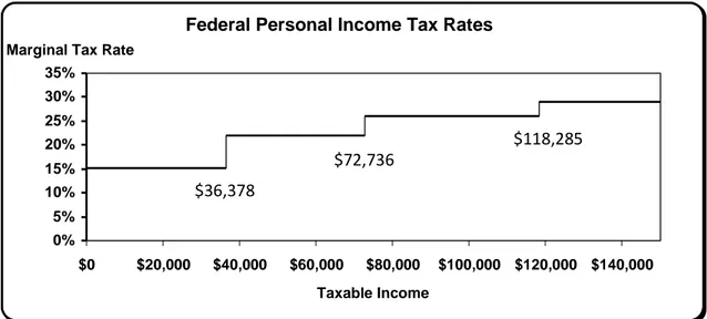
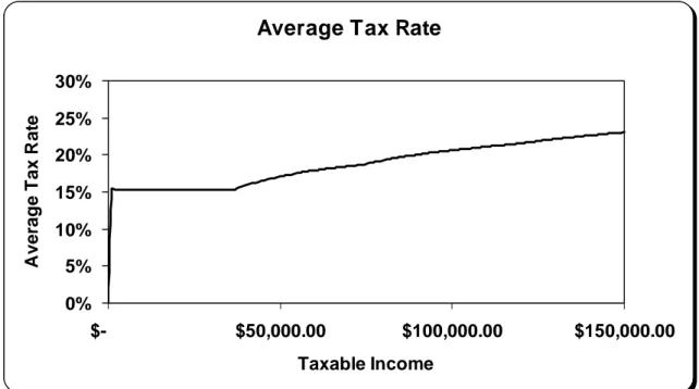
Under the 2006 federal income tax schedule, initial tax payable on taxable income was calculated using a series of different income brackets ($36,378 or less; more than $36,378 but not more than $72,756; more than $72,756 but no more than $118,285; and more than $118,285) taxed at different marginal tax rates (15.25%; 22%; 26%; and 29% respectively) (Figure 1). Using this simplistic schedule, the tax payable at specific levels of income can be calculated by finding the area under the rectangles and adding them up. For instance, for taxable income of $100,000, the tax payable is calculated as ($36, 378 * 0.1525) + ($36,378 * 0.22) + [($100,000 – $72,756) * 0.26)] = $20,634 (Figure 2). The actual calculation of the average or effective tax rate at this point is quite simple: (tax payable / taxable income) * 100 = average tax rate (ATR) in percentage. For this example: ($20,634 / $100,000) * 100 = 20.63, therefore 20.63% is the ATR for taxable income of $100,000 (before tax credits). If we graph the average tax rates for all levels of income, we instantly observe an increasing average tax rate at a slightly decreasing rate but only after a certain level of income (Figure 3). This is explained by the fact that for income falling within the first tax bracket, only the initial proportional (or flat) marginal tax rate applies. For this reason, the CRA introduces a basic personal amount of $8,839 (in 2006) to the equation taxed at the lowest marginal tax rate of 15.25%. Graphing this new function for average tax rates at different levels of income clearly displays a more progressive income tax structure (Figure 4). In this case, a person with a taxable income of $100,000 would calculate an average tax rate of 19.29% or owe $19,286 in tax payable after taking into account the basic personal amount.

3.2 Alternative Function Model

While the current bracket model respects some of the criteria for evaluating taxes such as fairness and vertical equity, it does seem a bit complicated, outdated and a far stretch for achieving a simple end; that is, making sure that people with more taxable income have higher average tax rates (progressive tax system).

(16)

8

Federal Personal Income Tax Rates

0% 5% 10% 15% 20% 25% 30% 35% $0 $20,000 $40,000 $60,000 $80,000 $100,000 $120,000 $140,000 Taxable Income

Marginal Tax Rate

$36,378

$72,736

$118,285

Source: Canada Revenue Agency. T1 – 2006, Federal Tax, Schedule 1.

Figure 1. 2006 Federal Income Tax Schedule.

0% 5% 10% 15% 20% 25% 30% 35% $0 $20,000 $40,000 $60,000 $80,000 $100,000 $120,000 $140,000 Taxable Income M ar g in al T ax R at e $5,548 $8,003 $7,083 = $20,634

(17)

9

Average Tax Rate

0% 5% 10% 15% 20% 25% 30% $- $50,000.00 $100,000.00 $150,000.00 Taxable Income A v er ag e T ax R at e

Figure 3. 2006 Federal Average Tax Rates.

Average Tax Rate (with BPA)

0% 5% 10% 15% 20% 25% 30% $- $50,000.00 $100,000.00 $150,000.00 Taxable Income A ver ag e T ax R at e

Source: Canada Revenue Agency. T1 – 2006, Federal Tax, Schedule 1

(18)

10

Option #1 – The Marginal Tax Function

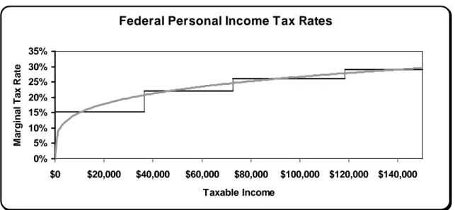
A simpler and more comprehensive model reaching the same objective would involve running an incremental marginal tax function crossing through all income tax brackets (Figure 5). This hypothetical curve was drawn using random trial and error numbers inspired by the structure of the classic Cobb-Douglas production function (Y = AKαL1-α). The resulting function reads as follows:

25 . 0 4

TI

c

MTR

=

[1]

MTR = Marginal Tax Rate TI = Taxable Income

c = 0.35 (where c is a constant)

0% 5% 10% 15% 20% 25% 30% 35% $0 $20,000 $40,000 $60,000 $80,000 $100,000 $120,000 $140,000 Taxable Income M a rg in al T a x R a te

Source: Author’s self-generated data.

Figure 5. Marginal Tax Function for Taxable Income.

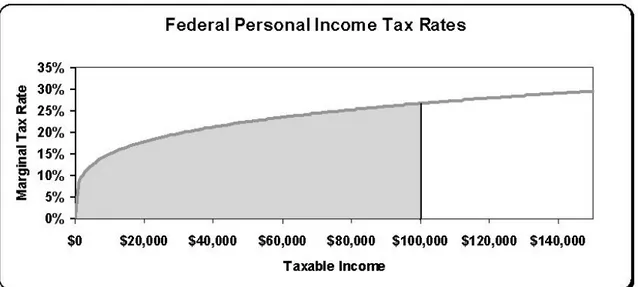
Furthermore, the net personal income tax payable at specific levels of income can also be easily calculated by finding the area under the curve of the proposed function (Figure 6) by calculating its integral:

) 012005 . 0 ( 1.25 TI PIT = × [2]

PIT = Personal Income Tax TI = Taxable Income

(19)

11

Figure 6. Area Under the Marginal Tax Curve Example.

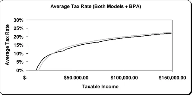
Again, illustrating the effect of the marginal function with the case of $100,000 taxable income; PIT = 0.012005 * $100,000^1.25 = $21,348. We can also calculate average tax rates for all levels of income using the marginal tax function, and this time, we instantly observe an increasing average tax rate at a slightly decreasing rate for all levels of income (Figure 7). It would be wise to point out that while the shape of the curve is drastically different from the bracket produced model, the average tax rate for a person with $100,000 in taxable income is 21.35% (a mere difference of 0.72% with the bracket model). Furthermore, once we adjust the function to include the basic personal amount as a non-refundable tax credit, both average tax rate curves closely resemble each other although the function curve is much smoother (Figure 8). The net personal income tax payable (before individual tax credits) can thus be found by calculating the area under the curve from the integral of the quadratic function and subtracting the basic personal amount claimed at the lowest marginal tax rate:

) ( ) 012005 . 0 ( 1.25 LMTR BPA TI PIT = × − × [3]

PIT = Personal Income Tax TI = Taxable Income

BPA = Basic Personal Amount LMTR = Lowest Marginal Tax Rate

(20)

12

Average Tax Rate (Marginal Tax Function)

0% 5% 10% 15% 20% 25% 30% 35% $- $50,000 $100,000 $150,000 Taxable Income A ver a g e T a x R at e

Figure 7. Average Tax Rate using the Marginal Tax Function.

Average Tax Rate (Both Models + BPA)

0% 5% 10% 15% 20% 25% 30% $- $50,000.00 $100,000.00 $150,000.00 Taxable Income A ver a g e T ax R at e

Figure 8. Average Tax Rates using Brackets and Marginal Tax Function models +

(21)

13

Finally, the average tax rate for a person with a taxable income of $100,000 becomes 20.00% (or $20,000 in net tax payable) under the marginal tax function when adjusting for the basic personal amount1_{. Again, this figure compares to the 19.29% average tax rate} calculated under the bracket model (variation of 0.71%).

Option #2 – The Average Tax Function

Drawing a random marginal tax curve and adjusting the parameters of the function until it closely resembles a target curve is one way for reaching a desired alternative function. However, we can also achieve similar results using a reversed engineering process. As it was mentioned, the new marginal tax function should essentially aim to reflect the current average income tax structure (including the basic personal amount – Figure 4). In order to achieve such a comparative functional model, a “curve fitting” procedure – such as a logarithmic model curve estimation regression – can be run through data of average tax rates using brackets (dependant variable: DV) and total income (independent variable: IV). For this purpose, 1,925 net income (pre-tax) amounts from Canadian tax filers were randomly selected from the Survey of Labour and Income Dynamics (SLID), 2003: Person file (Internet Data Library System, 2003). The range of net income was also artificially constrained between $0 and $150,000 by removing outliers. Using this data, the logarithmic model returns an R2 of 0.987***, suggesting that the average tax rate distribution is appropriately represented by the logarithmic function:

63 .

0 (ln)

072 .

0 ×

−

=

TI

ATR

[4]

ATR = Average Tax Rate TI = Taxable Income ln = Natural Logarithm

Once again, illustrating the effect of the average tax function with the case of $100,000 taxable income; ATR = 0.072 * (LN) $100,000 - 0.63 = 19.89%.2 Consequently, the net personal income tax payable at specific income levels can easily be calculated by multiplying the average tax rate by the total income (ATR * $100,000 = $19,893), thus the function:

[

TI

PIT

=

0 .

072 ×

(ln)

−

0 .

63 ]

×

[5]

1_{The small discrepancy with the amount reported by the bracket model can be attributed to estimation error of the marginal}

tax function ($20,000 - $19,286 = $714).

2

The logarithmic function returns a slightly higher average tax rate than the brackets model until $150,000 but it should be noted that the disparity increases significantly afterwards (reaching an ATR of 100% at ~ $10B/year).

(22)

14

PIT = Personal Income Tax TI = Taxable Income ln = Natural Logarithm

The small discrepancy ($19,893 - $19,286 = $607) with the amounts reported by the bracket model and logarithmic functions can be attributed to the curve estimation error incurred while running the regression. This error can be reduced by altering the equation parameters; however, such alterations would again fall into the political sphere.3

A major advantage of the logarithmic average tax function is that it makes the use of marginal income tax rates and the basic personal amount completely obsolete (as opposed to the brackets and marginal tax function models)4_{. In this case, the taxpayer could simply} input its taxable income into the logarithmic function [5] and the amount owed to the government for the given fiscal year (personal income tax) would be automatically calculated.

3_{It can be expected that a function (marginal tax + BPA or logarithmic average tax function) falling below all distribution}

points of the average tax rates as calculated by the tax brackets would be well received by many taxpayers.

4

The marginal tax function can also be seen as being independent from marginal tax rates but its PIT function essentially relies on the initial MTR function as well as the basic personal amount.

(23)

4. TAX FUNCTION BENEFITS

The previous section proved that it is indeed possible to construct a single tax function which would yield similar results as the current federal income tax brackets model. This in itself is not an achievement. Why should a government adopt such a model when there is no visible effect or clear advantage of doing so?

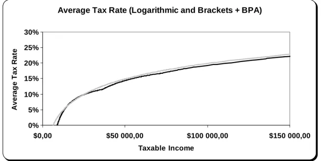
By now, it has been made clear that the federal income tax brackets and the marginal tax rates in Canada have been the subject of many debates over the past century and that the debates will most likely carry over through the next century. However, when targeting a given level of after-tax income distribution with the old fashioned tax structure, the different combination of income brackets and marginal tax rates (not including the basic personal amount) for achieving a target is practically endless. Using a single marginal or average tax function, the variables can be altered to make tax more or less progressive, to make the curve more or less concave, to make it decrease at a faster or slower rate, etc. All is needed is the adjustment of a few parameters in a simple quadratic or logarithmic function to reach an ideal equity tax structure. And while not introduced in this model, a parameter for full indexation could also be integrated within the function to address the issue of “creeping” due to inflation. In addition, a smooth marginal tax function instead of the current bracket model could also serve to increase tax efficiency by reducing the incentive for individuals to report lower personal income in order to fall into less heavily taxed income brackets. This in turn could potentially increase the tax compliance as the incremental marginal tax or average tax rates model could be perceived as being more equitable by the majority of taxpayers. This leads us to discuss the issue of visibility or transparency in light of the proposed personal income tax functions. Under the current federal income tax model, taxpayers are provided with a schedule that outlines marginal tax rates for each income bracket but which gives no indication of the average (or effective) tax rate for different levels of income. As we have seen before (Figure 3), the average tax rate distribution across levels of income does not seem nearly as fair until we add to it the basic personal amount calculation (Figure 4). This problem would be irrelevant with the use of a comprehensive marginal tax function that would clearly show the average tax rates for different levels of income in one graph (Figure 8) and even less so with the logarithmic average tax rate function (Figure 9).

(24)

16

Average Tax Rate (Logarithmic and Brackets + BPA)

0% 5% 10% 15% 20% 25% 30% $0,00 $50 000,00 $100 000,00 $150 000,00 Taxable Income A ver ag e T ax R at e

Source: Author’s self-generated data, Survey of Labour and Income Dynamics (SLID), 2003: Person file. Figure 9. Average Tax Rates using Logarithmic and Brackets + the Basic

Personal Amount models.

Finally, the proposed tax functions are not meant to be solve-all solutions for addressing the tax criteria discussed above. In fact, the only major advantage of using a function model rests in its flexibility of manipulation and goal targeting. Therefore, the purpose of this paper was not to argue for a specific tax reform but rather to provide politicians and policy-makers, as well as the general public, with a new tool for tampering with the tax system.

(25)

5. FURTHER CONSIDERATIONS

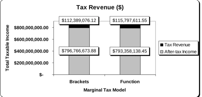
As outlined in the introduction, the proposed marginal tax model would require that everyone file their taxes online; that is, unless we want to teach people to use calculus or logarithmic functions to calculate their income taxes. However, filing taxes online does have advantages other than reducing administrative and personal opportunity costs. For one, the website (i.e. CRA NETFILE) could also serve as a platform for interactive learning of the tax system. Using the proposed marginal or average tax functions, the government could establish an interactive applet which people could use to harmlessly tweak parameters of the functions and watch their effect on the marginal and average tax curve. By combining the marginal and average tax database with a Lorenz curve (Figure 10) and tax revenue graph (Figure 11), the effects of the change in function parameters could also be seen on income inequality (as calculated by the Gini coefficient and illustrated by the Lorenz curve) and government tax revenues under different tax systems. This would help citizens see and understand the estimated impact of using different functions on post-tax income distribution, tax progressiveness and tax revenue for public spending. Furthermore, this interactive tool could also be reversed and used by politicians and policy-makers to derive optimal functions for reaching specific economic targets based on inequality and tax revenue indexes. However, as mentioned above, such a model would likely not survive on paper; and thus, online tax filing would be mandatory.

Finally, it is the author’s belief that personal income tax functions such as the ones presented in this paper have always been the underpinning ideal behind the personal income tax structure, and that major tax reforms have simply aimed to bring us closer to this ideal. This is yet another solution to bring us closer.

(26)

18

Source: Survey of Labour and Income Dynamics (SLID), 2003: Person file.

Figure 10. Example of Pre- and Post-Tax Lorenz Curve (Marginal Tax Function Model).

Tax Revenue ($) $793,358,138.45 $796,766,673.88 $112,389,076.12 $115,797,611.55 $-$200,000,000.00 $400,000,000.00 $600,000,000.00 $800,000,000.00 Brackets Function Marginal Tax Model

Tot a l Ta x a bl e I nc om e Tax Revenue After-tax Income

Source: Survey of Labour and Income Dynamics (SLID), 2003: Person file.

(27)

REFERENCES

Canada Revenue Agency (2006). General Income Tax Guide and Return. Federal Tax – Schedule 1. Available online at: http://www.cra-arc.gc.ca/E/pbg/tf/5000-s1/5000-s1-06e.pdf

Canada Revenue Agency (2007). NETFILE. E-services for individuals. Available online at: http://www.netfile.gc.ca/menu-e.html

Internet Data Library System (2003). Survey of Labour and Income Dynamics (SLID), 2003: Person

File. Available online at: http://janus.ssc.uwo.ca/idls/

Kesselman J. R. & Cheung R. (2004). “Tax incidence, progressivity, and inequality in Canada”,

Canadian Tax Journal, 52(3).

Kim,C. K. (2002). “Does fairness matter in tax reporting behavior?”, Journal of Economic

Psychology, 23(6), 771-785.

Organisation for Economic Co-operation and Development (2006). Policy Brief – Reforming Personal

Income Tax. Available online at: http://www.oecd.org/dataoecd/43/21/36346567.pdf

Rosen, H.S., Dahlby, B., Smith, R.S., & Boothe, P. (2002). Public Finance in Canada. Second

Canadian Edition. McGraw-Hill. Ryerson Limited.

Seidl, C., Topritzhofer, E., & Grafendorfer, W. (1970). “An outline of a theory of progressive individual income-tax functions”, Journal of Economics, 30(3), 407-429.

Tax Court of Canada (2002). History of the Tax of Canada. Available online at: http://www.tcc-cci.gc.ca/history_e.htm

The Canadian Institute of Chartered Accountants (2000). Fair, Timely, Sustainable: A framework for

personal income tax reduction in Canada. Available online at:

http://www.cica.ca/multimedia/Download_Library/Public_Affairs/Government_Affairs/Policy_Final _Nov26.pdf

Thinking outside the brackets : an alternative to the personal income tax brackets

INRS

Urbanisation, Culture et Société

Thinking Outside the Brackets:

An Alternative to the Personal Income Tax

Brackets

TABLE OF CONTENTS

TI

c

MTR

=

63

.

0

(ln)

072

.

0

×

−

=

TI

ATR

[

TI

TI

PIT

=

0

.

072

×

(ln)

−

0

.

63

]

×