HAL Id: tel-02612863
https://tel.archives-ouvertes.fr/tel-02612863
Submitted on 19 May 2020
HAL is a multi-disciplinary open access
archive for the deposit and dissemination of
sci-entific research documents, whether they are
pub-lished or not. The documents may come from
teaching and research institutions in France or
L’archive ouverte pluridisciplinaire HAL, est
destinée au dépôt et à la diffusion de documents
scientifiques de niveau recherche, publiés ou non,
émanant des établissements d’enseignement et de
recherche français ou étrangers, des laboratoires
On the multiphase structure of the turbulent neutral
interstellar medium
Antoine Marchal
To cite this version:
Antoine Marchal. On the multiphase structure of the turbulent neutral interstellar medium.
Astro-physics [astro-ph]. Université Paris-Saclay, 2019. English. �NNT : 2019SACLS249�. �tel-02612863�
Th
`ese
de
doctor
at
NNT
:2019SA
CLS249
On the multiphase structure of the
turbulent neutral interstellar medium
Th`ese de doctorat de l’Universit´e Paris-Saclay pr´epar´ee `a l’Universit´e Paris-Sud et au Commissariat `a l’´energie atomique Ecole doctorale n 127 Astronomie et Astrophysique d’Ile de France (AAIF)
Sp´ecialit´e de doctorat : Astronomie et Astrophysique
Th`ese pr´esent´ee et soutenue `a Gif-sur-Yvette, le 25 septembre 2019, par
ANTOINE
PAUL
HENRI
MARCHAL
Composition du Jury : Mathieu Langer
Professeur, Universit´e Paris-Sud Pr´esident
Robert Benjamin
Professor, University of Wisconsin Rapporteur
John Dickey
Professor, University of Tasmania Rapporteur
Naomi McClure-Griffiths
Professor, Australian National University Examinateur Franc¸ois Orieux
Maitre de conf´erence, Universt´e Paris-Sud Examinateur Benjamin Godard
Astronome-Adjoint, Ecole normale sup´erieure de Paris Examinateur Marc-Antoine Miville Deschˆenes
DR CNRS, Commissariat `a l’´energie atomique (AIM) Directeur de th`ese Patrick Hennebelle
Acknowledgement
First of all, I would like to thank my PhD supervisor, Marc-Antoine Miville-Deschênes, for guiding me during these three years. Our field of research, the interstellar medium, is simply fascinating. Many thanks for guiding me through this extremely rich literature. It would have been very easy for me to get lost otherwise. Finally, thank you for the many discussions we shared during this adventure. I try every day to be inspired by your enthusiasm and your overflowing scientific curiosity.
Je voudrais remercier très chaleuresement François Orieux pour m’avoir enseigné les outils dont j’avais besoin pour accomplir ce travail. Merci également à Charles Soussen pour ces excellents cours auxquels j’ai eu la chance d’assister. Merci à Marie-Jeanne Lesot, Adrien Revault d’Allonnes et Nicolas Gac pour toutes les riches discussions que nous avons eu lors de nos réunions hyperstars.
Many thanks to the members of my jury, Mathieu Langer, Robert Benjamin, John Dickey, Naomi McClure-Griffiths, François Orieux, Benjamin Godard and Patrick Hennebelle for evaluating this manuscript and for providing me with very constructive comments for its improvement. It was an honour for me to share this work with you, who have already advanced science so much.
Merci à l’Institut d’Astrophysique Spatial (IAS), au Commisariat à l’énergie atomique et aux énergies renouvelables (CEA) et aux équipes AMIS, COSM!X et LMPA de m’avoir acceuilli si chaleuresement. Un grand merci à Alain Abergel. Tu as été d’un grand soutien pour cette aventure.
Merci à tous les gens que j’ai rencontré et avec qui j’ai partagé ces trois belles années à l’IAS et au CEA. Merci Thomas, Victor, Thiébaut, Nadèje, Daniela, Raphaël, Adélie, Céline, Louis, Edouard, Lisa, Elena, Maximilien, Chiara, Baptiste, Solène, Anna, Rose, Ivan, Goeffrey, Geoffroy, Andrea, Adèle, Michelle ...
Merci à ma merveilleuse et grande famille, mon frère Louis, mes soeurs Jeanne et Léa, mes grands mères Elisabeth et Andrée, et mes parents Alexandre et Isabelle. Merci également à Julien, Pierre, Mélodie, Anne et Michel.
Merci à mes amis proches, Julien-Pierre qui m’a guidé vers la recherche, Bertrand, Arthur, Camille, Youri, Alexis, Tom, Steven, Melissa, Maximilien, Misha, Thiébaut, Thomas, Marie et Nilaï pour votre soutien.
Merci Wenjia. Merci d’être là et mille mercis pour ton grand soutien lors de l’écriture de ce manuscript.
À mon grand-père, Michel Marchal.
Contents
1 Introduction 1
2 Interstellar turbulence 5
2.1 Fluid mechanics . . . 6
2.1.1 The Navier-Stokes equation . . . 6
2.1.2 Kinetic energy equation . . . 8
2.1.3 Vorticity dynamics . . . 9
2.1.4 The closure problem of turbulence . . . 10
2.2 Reynolds’s experiment . . . 12
2.3 The phenomenology of Richardson and Kolmogorov . . . 13
2.4 Statistical properties of turbulence . . . 16
2.4.1 Spectral tensor . . . 16
2.4.2 Second order velocity structure function . . . 17
2.5 Turbulence in the ISM . . . 19
2.5.1 Beyond the incompressible turbulence . . . 19
2.5.2 Energy injections . . . 19
2.5.3 Observations of interstellar turbulence . . . 20
3 The neutral interstellar medium 23 3.1 Introduction . . . 24
3.1.1 Prediction and detection . . . 24
3.1.2 Early work . . . 24
3.2 Thermal instability . . . 25
3.2.1 The energy equation . . . 25
3.2.2 Perfect gas . . . 26
3.2.3 Equilibrium state and perturbation . . . 27
3.2.4 Static scale . . . 29
3.2.5 Dynamical scales. . . 29
3.3 Heating and cooling processes . . . 30
3.3.1 Photoelectric heating from small grains and PAHs . . . 31
3.3.2 Cooling and recombination . . . 32
3.3.3 Thermal equilibrium . . . 34
3.4 Thermal structure of the neutral ISM . . . 34
3.5 Morphological structure of the neutral ISM . . . 35
3.5.1 Mapping the neutral ISM. . . 35
3.5.2 Vertical structure . . . 36
3.5.3 HI shells. . . 38
3.5.4 Intermediate and high velocity clouds . . . 41
3.6 Turbulence in the neutral ISM . . . 44
4 ROHSA : Regularized Optimization for Hyper-Spectral Analysis 47 4.1 Methodology . . . 48
4.1.1 Gaussian decomposition of the 21 cm emission. . . 48
4.1.2 Limitation of the Gaussian model . . . 49
4.1.3 Development of a new approach . . . 49
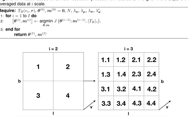
4.1.4 ROHSA . . . 50
4.2 Evaluation on numerical simulation . . . 54
4.2.1 Numerical simulation. . . 54
4.2.2 21cm line synthetic observations . . . 54
4.2.3 Results . . . 57
4.3 Application on high-latitude HI gas . . . 66
4.3.1 North ecliptic pole . . . 67
4.3.2 Results . . . 69
4.4 Discussion . . . 73
4.5 Summary . . . 78
5 North Ecliptic Pole : A new window on the multiphase neutral ISM 79 5.1 North ecliptic pole . . . 80
5.1.1 General description . . . 81
5.1.2 Integrated density fields of local gas . . . 81
5.1.3 Mass fractions of local gas . . . 84
5.2 Spatial distribution of the gas along the line of sight. . . 85
5.2.1 Emission from the Local Interstellar Cloud (LIC). . . 85
5.2.2 Beyond the Local Interstellar Cloud. . . 86
5.3 Disentangling thermal and turbulent velocity dispersions in the WNM . . . 89
5.3.1 Use of CNM structures as tracer particles . . . 89
5.3.2 Use of the centroid velocity field of the WNM . . . 90
5.4 Volume filling factors . . . 93
5.4.1 Filling factor of the multiphase HI . . . 94
5.4.2 Impact from diffuse ionized gas . . . 96
5.5 Thermodynamics and turbulence of the WNM . . . 96
5.5.1 Thermodynamic properties . . . 96
5.5.2 Properties of the turbulent cascade. . . 98
5.5.3 Thermal condensation of the WNM in NEP . . . 102
5.6 Discussion . . . 103
5.7 Summary . . . 104
6 Conclusion and perspectives 105 Appendix A Spatial power spectrum analysis 109 A.1 Spatial power spectrum of the column density field . . . 109
A.2 Impact of volume filling factor on the statistics of projected quantities . . . 112
A.2.2 Velocity field . . . 115
Appendix B Publication in Astronomy & Astrophysics 117
B.1 ROHSA : Regularized Optimization for Hyper-Spectral Analysis - Application to phase separation of 21 cm data . . . 117
Bibliography 139
1
Introduction
General context According to human conception, the Universe is almost empty. In the heart of galaxies, the average density of gas is about one particle per cubic centimetre. Brought back to sizes that the human mind can conceive, it would be necessary to fill the volume occupied by the earth with only a few liters of water to obtain the same value (Christopher McKee interview, 2014). It is because of its immensity, just as inconceivable to the human mind as its density, that the Galaxy draws all its baryonic mass. Like for the Universe as a whole, the hydrogen atom is the most abundant element in galaxies, being in neutral (HI), ionized (HII) or molecular (H2) form. It is from these states that the modern theory of the interstellar medium emerged, grouping together a total of five distinct phases. From the hottest to the coldest phase, the first of these is the hot ionized medium (HIM), an ionized gas with temperatures& 106K and densities. 0.003 cm≠3. This phase, also called the hot corona, is mainly heated by supernovae explosions. The second is the warm ionized medium (WIM). Having temperatures of ≥6000-12000 K, this diffuse gas is primarily ionized by UV photons emitted by O and B stars in the Galaxy. The third and fourth are the warm neutral medium (WNM) and cold neutral medium (CNM). Temperatures and densities of these two phases can vary considerably, from ≥50 to 8000 K and ≥0.5 to 50 cm≠3. The fifth and last is made of molecular clouds whose temperatures are typically ≥10-20 K and densities & 103cm≠3. Interestingly, these phase are roughly in pressure equilibrium and the vertical thickness of each phase increases with temperature. Despite this pressure equilibrium on large scale, the Milky Way is a system that is highly out-of-equilibrium from a dynamical point of view. All the phases appear to be in constant interaction.
Among these interactions, the accretion of neutral gas from the Galactic halo is of primary interest. A major component of the neutral ISM (WNM+CNM) is a population of clouds, named High-Velocity Clouds (HVCs), which are located in the Galactic corona. These structures are falling into the gravitational potential of the Milky Way, providing gas supply to the star formation. In the Galactic plane, the neutral and molecular phases are particularly interesting for understanding the star formation cycle in galaxies. Stars form by gravitational collapse of dense and cold structures located in molecular clouds. However, the process that leads to the formation of these over-densities is still unclear. It is believed that the radiative condensation of the diffuse WNM to produce a thermally unstable lukewarm medium and a dense cold medium is closely related to the initial step leading the atomic-to-molecular (HI-to-H2) transition and the formation of molecular clouds. Huge efforts have been made to understand this transition, but the step that led to the formation of the cold HI still remains unclear. In particular, one key element to understand the star formation cycle seems to be related to the efficiency of formation of this cold HI (Ostriker et al., 2010), whether it is form in the Galactic disk or accreted from the Galactic halo (HVCs).
The current vision of this condensation process from the warm to the cold phase has a long history. Early observations of the 21 cm line showed a significant difference between emission and absorption spectra. On lines of sight to radio-sources, the HI appears in absorption with very narrow features
(a few km s≠1). In emission the 21 cm line contains these narrow features on top of much boarder spectral structures (10-20 km s≠1).Clark (1965)was the first to suggest that this might be the signature of a cloud-intercloud medium in pressure equilibrium. Very rapidlyField (1965)andField et al. (1969) introduced the concept of thermal instability and laid out the theoretical ground of a "two phase" HI model showing that, at the pressure of the ISM, the heating and cooling processes naturally lead to two thermally stable states: a dense cold neutral medium (CNM - T ≥ 50 K, n ≥ 50 cm≠3) immersed in a diffuse warm neutral medium (WNM - T ≥ 8000 K, n ≥ 0.3 cm≠3). This view was later complemented byWolfire et al. (1995)andWolfire et al. (2003)who considered updated heating (dominated by the photo-electric effect on small dust grains) and cooling (dominated by CII - 158 µm, OI - 63 µm, L– and electron recombinations onto positive charged grains) processes of the ISM.
This description of the diffuse neutral gas complemented a parallel hypothesis that emerged in the 1950s (e.g.,Weizsäcker, 1951;Hoerner, 1951;Chandrasekhar and Münch, 1952) and considered the ISM as a multi-scale turbulent medium. In this case, the density and velocity structures are the result of a highly dynamical and out-of-equilibrium medium. In order to reconcile the ‘static/two-phase’ and the ‘turbulent’ hypotheses, several studies have aimed at understanding the production of the CNM in a turbulent and thermally unstable flow using numerical simulations (e.g.,Hennebelle and Pérault, 1999;Koyama and Inutsuka, 2002;Audit and Hennebelle, 2005;Hennebelle et al., 2008;Saury et al., 2014). In general, these numerical studies show that the WNM has the properties of a trans-sonic turbulent flow, while the CNM shows a much more contrasted density structure, in accordance with the cloud-intercloud picture. In addition, such studies indicate the presence of a significant fraction of the mass being in the thermally unstable regime (i.e., with a temperature mid-way between the CNM and WNM stable states). For instance,Saury et al. (2014)showed that 30% of the HI is in the thermally unstable regime. Interestingly, these latter authors also show that this lukewarm neutral medium (LNM) is spatially located around the cold structures, pointing at the transitional nature of this thermal state. From an observational standpoint, studies combining 21 cm absorption and emission data have clearly revealed the presence of HI at intermediate/unstable temperatures, typically between 500 and 5000 K (e.g.,Heiles and Troland, 2003b;Kanekar et al., 2003;Roy et al., 2013a;Roy et al., 2013b;Murray et al., 2015;Murray et al., 2018b). Based on a coherent modeling of emission and absorption spectra, Heiles and Troland (2003),Murray et al. (2015)andMurray et al. (2018)estimated that about 30% of the HI is in the cold CNM phase, 20% in the thermally unstable regime, and 50% in the WNM. Nevertheless the fraction of the HI in each phase remains uncertain and large variations are observed: the fraction of the mass in the CNM ranges from ≥1% to more than 50% (Murray et al., 2018b). Motivation The nature of these variations and how they relate to the dynamical conditions of the gas remains largely unexplored from the observational point of view. One main hurdle in getting access to this information is the fact that our knowledge of the multiphase nature of the HI relies on 21 cm absorption measurements that are limited to lines of sight to radio sources. By construction, this way of observing prevents us from mapping the HI phases. To go further, and really compare with numerical simulations that are currently under-constrained by observation, it is necessary to map the column density structure of each phase and study the spatial variations of their centroid velocity and velocity dispersion. This calls for methods that can extract the information of each HI phase from fully sampled 21 cm emission data only. Huge efforts have been made to map the 21 cm emission of the Galactic HI (recent examples are Taylor et al., 2003; Kalberla et al., 2005; Stil et al., 2006;
McClure-Griffiths et al., 2009;Winkel et al., 2016;Peek et al., 2018) and a large amount of data is now available. The information about the multiphase and multi-scale nature of the HI contained in these large hyper-spectral data cubes has remained elusive due to the difficulty in separating the emission from the different phases on each line of sight. The work presented in this thesis aims to develop a new tool capable of extracting this information from the 21 cm emission data only. The second objective of this work is to use this new algorithm to study the thermal and turbulent properties of the neutral interstellar medium, especially in the WNM where very little information have been obtained to date. Thesis structure Chapter2is dedicated to giving the reader a brief introduction to fluid mechanics and turbulence. The Navier-Stokes equations are used to present and discuss the concept of turbulence. Some historical experiments and concepts related to turbulence are presented in parallel in order to understand the emergence and evolution of this discipline of primary interest for astrophysics. Tools to analyze statistical properties of turbulence are then presented. Finally, the specific case of interstellar turbulence and the mechanisms that generate it at all scales of the interstellar medium are discussed, as well as the application of the statistical tools presented for the study of interstellar turbulence. Chapter3provides a brief historical overview of the detection and early works related to interstellar neutral hydrogen. The main steps in the calculation of thermal instability are presented as well as the heating and cooling processes necessary to understand the growth of perturbations that cause the thermal condensation of the fluid. Then, an observational overview of the thermal and morphological structure of the neutral ISM is presented in order to establish the environments in which this phase transition occurs in the interstellar medium. This variety of object and medium will allow us in particular to highlight the major stakes that the separation of the phases of the interstellar medium represents. The goal of Chapter4is to present a new algorithm developed to perform the separation of diffuse sources in hyper-spectral data. Specifically, the algorithm is designed in order to address the velocity blending problem by taking advantage of the spatial coherence of the individual sources. The main scientific driver of this effort was to extract the multiphase structure of the HI from 21 cm line emission only, providing a means to map each phase separately, but the algorithm developed here should be generic enough to extract diffuse structures in any hyper-spectral cube. This new Gaussian decomposition algorithm named ROHSA (Regularized Optimization for Hyper-Spectral Analysis) is based on a multi-resolution process from coarse to fine grid. ROHSA uses a regularized nonlinear least-square criterion to take into account the spatial coherence of the emission and the multiphase nature of the gas simultaneously. In order to obtain a solution with spatially smooth parameters, the optimization is performed on the whole data cube at once. The performances of ROHSA are tested on a synthetic observation computed from numerical simulations of thermally bi-stable turbulence. We then apply ROHSA to a 21 cm observation of a region of high Galactic latitude from the GHIGLS survey and present our findings.
Chapter5is dedicated to the study of the different inter-connected properties of the diffuse neutral ISM, namely the thermal properties, the statistical properties of the turbulent cascade acting in the fluid, and the properties of the condensation mode of the thermal instability allowing the formation of the dense neutral phase. For this analysis we use the same region of high Galactic latitude from the GHIGLS survey as presented in Chapt.4. In particular, the goal of this chapter is to analyze these properties in
the vicinity of the Sun, at the border of the Local Bubble. The studied field is therefore chosen in order to focus only on the local velocity component (LVC) of the emission.
2
Interstellar turbulence
„
Eddie:You know, it’s funny... you come to someplace new, an’... and everything looks just the same.
Willie:
No kiddin’ Eddie.
— Stranger than Paradise (1984) Jim Jarmusch
Contents
2.1 Fluid mechanics . . . 6
2.1.1 The Navier-Stokes equation . . . 6
2.1.2 Kinetic energy equation . . . 8
2.1.3 Vorticity dynamics. . . 9
2.1.4 The closure problem of turbulence. . . 10
2.2 Reynolds’s experiment. . . 12
2.3 The phenomenology of Richardson and Kolmogorov . . . 13
2.4 Statistical properties of turbulence . . . 16
2.4.1 Spectral tensor . . . 16
2.4.2 Second order velocity structure function. . . 17
2.5 Turbulence in the ISM . . . 19
2.5.1 Beyond the incompressible turbulence . . . 19
2.5.2 Energy injections . . . 19
2.5.3 Observations of interstellar turbulence . . . 20
2.1
Fluid mechanics
This section is dedicated to giving the reader a brief introduction to the concept of turbulence emerging from fluid mechanics, by limiting ourselves to incompressible flows1. The equations presented here are
largely taken from the following book: "turbulence, an introduction for scientist and engineers" of P. A. Davidson (Davidson, 2015). In this short overview, we derive the Navier-Stokes equation and the kinetic energy equation to establish the expression of the internal energy transfer rate which is of primary interest for describing the turbulence cascade acting in the ISM. We finally introduce the concept of turbulence by making a brief description of vorticity dynamics. For complementary discussions of these equations, we refer the reader to the Chapter 2 ofDavidson (2015).
2.1.1
The Navier-Stokes equation
The continuity equation First, let us consider a fluid element of volume ”V with a density fl, moving at a local velocityu. Its mass is
”m= fl”V. (2.1)
Assuming that this mass is conserved, its time-rate-of-change is zero and we have D(”m)
Dt = 0. (2.2)
Combining Eqs.2.1and2.2, we have Dfl Dt + fl 5 1 ”V D(”V ) Dt 6 = 0 (2.3)
where the term in bracket is the time rate of change of the volume of the fluid element, per unit volume. It can be easily shown (see Sect. 2.4 of Anderson (1995)) that it is the physical meaning of the divergence of the velocity Ò · u. Equation2.3becomes
Dfl
Dt + flÒ · u = 0. (2.4)
This is the continuity equation. In the case of an incompressible fluid, Eq.2.4reduces to
Ò · u = 0. (2.5)
The momentum equation The Newton’s second law applied to the same fluid element can be written in the form
(fl”V )Du
Dt = ≠ (Òp) ”V + viscous forces (2.6)
where the first term on the right hand is the net pressure force acting on the fluid element and the second term represents the forces arising from the viscous stresses2. The viscous stresses are 1It is now well known that turbulence in the interstellar medium is far from being considered incompressible. Nevertheless,
this framework allows us to first understand the fundamental principles related to turbulence.
composed of shear stresses and normal stresses that, if we consider a cubic fluid element, are noted ·xy, ·xz, ..., ·xx, ·yy and ·zz. Any imbalance in stress arising between faces of a fluid element implies a net viscous force. As a result, the fluid element experiences a deformation that leads to a change in its trajectory. The viscous force in each direction i of the cube is then proportional to the sum of the variation of stresses (dependent of i) between the top and the bottom of each faces. Following the summation over repeated index i and j (convention), the viscous forces are
fi= ˆ·ji
ˆxj
”V. (2.7)
Combining Eqs.2.6and2.7, we obtain flDu
Dt = ≠ Òp + ˆ·ji
ˆxj. (2.8)
We shall now use Newton’s law of viscosity (shear stress is directly proportional to velocity gradient) to link ·ij to the rate of deformation of the fluid element:
·ij = fl ‹ ;ˆu i ˆxj + ˆuj ˆxi < . (2.9)
Note that the coefficient of proportionality is simply the absolute viscosity µ=fl‹, where ‹ is the kinematic viscosity of the fluid. Physically, we can get an idea of what a viscous stress represents by considering a shear flowu=(ux(y),0,0). Each layer of fluid slides over each other, causing a deformation of fluid elements. In this case, the viscous stress ·yxis proportional to a rate of sliding (or distortion rate) which is simply the velocity gradient ˆux
ˆy and the coefficient of proportionality is the absolute viscosity µ of the fluid. Introducing the strain-rate tensor Sij
Sij =12 5ˆu i ˆxj + ˆuj ˆxi 6 (2.10) we rewrite ·ij in its well-know compact form
·ij = 2fl‹Sij (2.11)
Substituting Eq.2.11in Eq.2.8with fl constant, we obtain the so-called Navier-Stokes equation Du Dt = ≠ Ò 3p fl 4 + ‹ Ò2u (2.12)
Note that Eq.2.12is expressed using the convective derivative D( )/Dt used in Eq.2.3, that takes into account both temporal and spatial variations of each component of the vector fieldu. The convective
derivative can be developed using the chain rule (see Sect. 2.1.2 ofDavidson (2015)) to obtain an explicit formula of the acceleration of the fluid element
Du Dt =
ˆu
ˆt + (u . Ò) u (2.13)
The Navier-Stokes equation presented in Eq.2.12then becomes ˆu ˆt + (u . Ò) u = ≠ Ò 3p fl 4 + ‹ Ò2u (2.14) 2.1 Fluid mechanics 7
We can already note that terms(u . Ò) u and ‹ Ò2u of Eq. 2.14can be, respectively, seen as an advection term and a diffusion term. We will see in the following Sect.2.2that the development from a laminar to a turbulent regime depends on the ratio of these two terms, defined as the Reynolds number Re. It is important to note here that the advection term is quadratically non-linear inu. It is via this non-linearity that instabilities can grow and eventually, if Re is sufficiently high, cause turbulence.
The energy equation The third and last fundamental equation of fluid mechanics results from the first law of thermodynamics: the total energy of the moving fluid element is conserved. However, its derivation is not of primary interest for the present chapter and we shall come back to it in the following Chapt.3to understand the concept of thermal instability in astrophysical plasma. Instead, we focus here on the kinetic energy equation which allows us to introduce the concept of dissipation of mechanical energy per unit of mass.
2.1.2
Kinetic energy equation
Let us now derive the kinetic energy equation by multiplying Eq.2.12byu u .Du Dt = D Dt 3 u2 2 4 = ≠ Ò .5pflu6 + ‹ u .!Ò2u" (2.15) The second term of the right hand side of Eq.2.15can be decomposed as
‹u .!Ò2u" = ui ˆ
ˆxj [·ij/ fl] = ˆ
ˆxj [ui·ij/ fl] ≠ 2‹SijSij. (2.16) Equation2.15then becomes
ˆ!u2/2" ˆt = ≠ Ò . #! u2/2 + p/fl" u$ ≠ ˆ ˆxj [ui ·ij/ fl] ≠ 2‹SijSij. (2.17) Integrating Eq.2.17over an arbitrary volume V gives
d dt ⁄ V ! u2/2" dV = ≠ ⁄ V Ò . #! u2/2" u$ dV ¸ ˚˙ ˝
- (rate at which kinetic energy is transported across the boundary)
(2.18)
≠ ⁄
V Ò . [(p/fl) u] dV
¸ ˚˙ ˝
+ (rate at which the pressure forces do work on the boundary)
(2.19) ≠ ⁄ V ˆ ˆxj [ui ·ij/ fl] dV ¸ ˚˙ ˝
+ (rate at which the viscous forces do work on the boundary)
(2.20) ≠ ⁄ V 2‹SijSijdV ¸ ˚˙ ˝
+ (rate of loss of mechanical energy to heat)
where the meaning of the last term of the right hand side is directly inferred from the conservation of energy. When applied to a small volume ”V , this term is the dissipation of mechanical energy per unit of mass and is noted
‘= 2‹SijSij. (2.22)
This quantity is of primary interest since, as we will see in the following Sect.2.3, it allows one to characterize the turbulence cascade acting in the fluid. It is also possible, after some algebra, to write the total rate of dissipation of mechanical energy as function of the curl of the velocity fieldu
⁄
‘dV = ‹ ⁄
(Ò ◊ u)2dV = ‹⁄ Ê2dV (2.23)
where Ê=Ò ◊ u is the vorticity field. We can anticipate via this result that the vorticity field Ê plays an important role in describing the properties of a turbulent flow since it is directly related to the rate of dissipation of mechanical energy. Note that Ê can be seen as a measure of the local rotation of a fluid element. Therefore, a fluid element can be distorted/strained at a rate Sij and rotated at a rate Ê.
These two quantities are naturally linked by the gradient of the velocity field at any point in the fluid ˆui ˆxj = 1 2 3ˆu i ˆxj + ˆuj ˆxi 4 + 123ˆui ˆxj ≠ ˆuj ˆxi 4 = Sij ≠ 12‘ijkÊ (2.24) where ‘ijkis the Levi-Civita symbol.
2.1.3
Vorticity dynamics
The idea that the vorticity field plays an important role in describing turbulence can be exploited by looking at its dynamics. In particular, we shall compare in this section the behaviour of governing equations of velocity and vorticity fields. This comparison will allow us to develop a first definition of turbulence.
Let us write its governing equation3
ˆÊ
ˆt = Ò ◊ [u ◊ Ê] + ‹Ò
2Ê (2.25)
that can also, using the identity
Ò ◊ (u ◊ Ê) = (Ê . Ò) u ≠ (u . Ò) Ê (2.26)
be rewritten as
DÊ
Dt = (Ê . Ò) u + ‹Ò
2Ê. (2.27)
It is important to note that unlike the governing equation of the velocity fieldu expressed in Eq.2.14, Eq.2.27is only composed of a diffusion term and a term of creation of vorticity fuelled by variations of the velocity field along the vorticity tubes, and that these two mechanisms are local. Therefore, unlike the velocity field, the vorticity can only be locally spread.
3The vorticity equation can be easily obtained by rewriting Eq.2.14using the identity Ò!u2/2"=(u . Ò) u + u ◊ Ê and by
taking its curl.
To understand why the evolution of velocity field is non-local, it is useful to compare Eqs.2.14and2.27
which respectively are the governing equations of the velocity fieldu and the vorticity field Ê. The main
difference between Eqs.2.14and2.27is that the governing equation of the velocity field contains the term ≠Ò (p/fl). To better understand its nature and impact on the fluid, we can take the divergence of Eq.2.12. In this way, we can relate directly the pressure field to the velocity field. It follows
Ò2(p / fl) = ≠ Ò . (u . Òu) (2.28)
that can be reversed using the Biot-Savart law, giving p(x) = fl
4fi⁄ [Ò. (u.Òu)] Õ
|x ≠ xÕ| dxÕ. (2.29)
The pressure field can be calculated at every point of space using the velocity fieldu. An important
property of incompressible fluid is that pressure waves travel at infinite speed. The information contained in p(x) is therefore instantaneously transferred to the entire fluid. It makes the pressure field a non-local one, unlike the vorticity field Ê. In other words, any modification ofu in space is instantaneously felt by
the fluid whose response is controlled, again at any point in space, by the term ≠Ò (p/fl) in Eq.2.14. This instantaneous propagation of the information makes a representation ofu impossible in terms of
sub-regions of the fluid. On the other hand, it is natural to think about the vorticity field as a group of local regions called vortices evolving together in space. In general, these vortices are called "eddies". FollowingDavidson (2015), we shall now be able to define turbulence, as suggested by Stanley Corrsin in 1961, by the following
Incompressible hydrodynamic turbulence is a spatially complex distribution of vorticity which advects itself in a chaotic manner in accordance with Eq.2.27. The vorticity field is random in both space and time, and exhibits a wide and continuous distribution of length and time scales.
2.1.4
The closure problem of turbulence
We have seen previously that the pressure p can be determined instantaneously using the velocity field u using Eq.2.29. It therefore appears that for incompressible flows, the Navier-Stokes equation presented in Eq.2.14is not anymore a function of p andu but can be formally written as
ˆu
ˆt = F (u) (2.30)
where F(u) contains the inertial, pressure and viscous forces. It turns out that Eq.2.30is deterministic and can be solved over time to obtainu(x, t). So why is it well known that "turbulence is the most
unsolved problem of classical physics" (Richard Feynman) ? The answer to that question is called the closure problem. Because of the chaotic behaviour ofu(x, t) in the turbulent regime, most of
the turbulence theories developed so far are based on statistical modelling, involving the Reynolds decomposition
Fig. 2.1.:Plots of parts of Reynolds decomposition. From Introductory Lectures on Turbulence: Physics, Mathe-matics and Modeling (James M. McDonough)
Fig. 2.2.:Sketch of the transition from laminar (top) to turbulent flow (middle) fromReynolds (1883). The bottom panel shows the same turbulent flow when observed with the light of an electric spark to reveal the "eddies" (now viewed as vorticies) of the flow.
whereu is the mean flow and uÕis a random fluctuation also called the "fluctuating part". Figure2.1 shows a sketch of the temporal evolution ofu(x) and uÕ(x, t). The traditional way of solving Eqs.2.14
Fig. 2.3.:Drawing made by Leonardo da Vinci (circa 1510) about the movement of water.
statistically is by using a decomposition of the form of2.31involving in particular the two-point and three-point correlation function4. The formulation of an equation of the three-point correlation function
involves the four-point correlation function, and so on. The set of equations inferred from this method is therefore not a closed system. It turns out that it is a direct consequence of the non-linearity of the term(u . Ò) u, which is also mostly responsible for the development of turbulence. Therefore, no exact solution can be found for the velocity fieldu(x, t) in space and time, even when considering its
statistical properties. We will limit ourselves here to mentioning that a wide variety of approximations have been developed to close this system since the first try by Joseph Valentin Boussinesq at the end of the nineteenth century.
2.2
Reynolds’s experiment
Now that we have an idea of the equations that govern incompressible fluids, we can ask ourselves under what precise conditions turbulence develops to form this collection of "eddies" called vortices ? Or in other words, under what conditions do we switch from a laminar regime to a turbulent regime ? Osborne Reynolds, in 1883, was the first to address the question by studying a simple flow passing through a pipe. The sketch of his experiment is shown in Fig.2.2where the top and middle panels represent the laminar and turbulence cases. He argued that the transition of turbulence represented here depends on the viscosity ‹ of the fluid, the velocity u of the flow and the diameter d of the pipe
which corresponds to the characteristic length l of the flow. The dimensionless combination of these quantities is now called the Reynolds number Re
Re=ul
‹ . (2.32)
Reynolds found that turbulence appears at Re ≥2000 if initial perturbations applied to the flow are not too small. On the other hand, when minimizing these perturbations, the flow can remains in a laminar regime up to Re ≥ 13 000. This wide range over which turbulence may eventually appear highlights the crucial role played by the amplitude of initial disturbances.
A modern interpretation of the Reynolds number can be obtained with a simple dimensional analysis of the ratio of the advection term and the diffusion term of Eq.2.14. Using the characteristic length l of the system, the ratio is approximately
(u . Ò) u ‹Ò2u ≥ u2/l ‹u/l2 = ul ‹ = Re (2.33)
As shown in Fig.2.2(bottom), when observed with the light of an electric spark, the turbulent regime described by Reynolds results in a collection of "eddies" (vorticies). It is interesting to note, however, that the first visual representation of a turbulent flow should be attributed to Leonardo da Vinci (≥1510) whose infinite detail drawing shown in Fig.2.3exhibits a complex collection of "eddies" emerging from a laminar flow of water. It is also astonishing to read the annotation associated to the drawing,
Observe the motion of the surface of the water which resembles that of hair, and has two motions, of which one goes on with the flow of the surface, the other forms the lines of the eddies; thus the water forms eddying whirlpools one part of which are due to the impetus of the principal current and the other to the incidental motion and return flow.
which is reminiscent of Eq.2.31.
2.3
The phenomenology of Richardson and Kolmogorov
One striking thing that appears when you look at da Vinci’s drawing is the variety of size of the eddies. It is now well known, as we will see in the following, that the size of the largest eddies is comparable to the characteristic length l of the flow and the size of the smallest eddies depends on the Reynolds number Re. It was by attempting to describe the properties of this variety of "eddies" that Richardson introduced the concept of energy cascade at high Re. His commentary on the behaviour of clouds in the atmosphere (1922) is probably the most quoted since the emergence of turbulence theories.
One gets a similar impression when making a drawing of a rising cumulus from a fixed point; the details change before the sketch can be completed. We realize that big whirls have little whirls that feed on their velocity, and little whirls have lesser whirls and so on to viscosity. The idea has evolved since 1922, thanks in particular to Geoffrey Ingram Taylor and Andrey Nikolaevich Kolmogorov, whose contributions allow us to express the modern vision of this energy cascade.
When instabilities are generated on a large scale in the flow, this creates eddies (a collection of vortices). These coherent structures in space can then themselves be subject to new instabilities, which cause the transfer of their respective energies (ideally without creation or destruction because the viscous stresses acting on large scales are negligible) to smaller scales. In other words, the eddies break into smaller ones. The same process of energy accumulation subjected to new instabilities generates a new transfer on a lower scale and so on until the viscous forces become dominant (i.e. Re ≥1) and dissipate the energy.
This vision of the energy cascade led Kolmogorov to introduce in 1941 the two following hypothesis: 1. At sufficiently high Reynolds numbers, there is a region of high wave numbers, where the
turbulence is statistically in equilibrium and uniquely determined by the dissipation of mechanical energy per unit of mass ‘ and the viscosity of the fluid ‹. This state of equilibrium is universal and at this state, the turbulence is statistically homogeneous and locally isotropic.
2. At sufficiently high Reynolds numbers, the statistics of the motions of scale l in the range l0π l π ÷ have a universal form that is uniquely determined by the dissipation of mechanical energy per unit of mass ‘, independent of the viscosity of the fluid ‹.
These are now called Kolmogorov’s hypothesis. The range l0π l π ÷ is called the inertial range where l0is the integral length scale and ÷ is the Kolmogorov length scale. In other words, it corresponds to the range of scales where the statistical properties of the flow are self-similar. Having this in mind, it is now possible with a simple dimensional analysis to determine the dissipation scale ÷ of the flow. Let us consider the turn-over time ·l0=l0/u0of the largest eddies which correspond approximately to their
timescale or lifespan. The rate of energy per unit mass transferred to the next lower scale is then ≥ u20/(l0/u0) = u30/l0. (2.34) This was introduced by Taylor in 1935, whose idea was that a large eddy loses a significant fraction of its kinetic energy within one eddy turn-over time. Considering now the velocity of the smallest eddies v, the rate of dissipation associated is given by Eq.2.22and can be approximated using Sij ≥ v/÷ as
‘≥ ‹SijSij ≥ ‹(v2/÷2). (2.35)
The energy cascade as expressed above (no accumulation of energy at any intermediate scale, i.e. statistically steady turbulence) implies that the energy transfer rate is constant over scales and so =‘,
u3/l≥ ‹(v2/÷2). (2.36)
Knowing that the Reynolds number on the dissipation scale is
Re÷= v÷/‹ ≥ 1, (2.37)
We obtain the following relations
÷≥ l0Re≠3/4≥ (‹3/‘)1/4 (2.38)
and
Fig. 2.4.:FromSaury (2012): Sketch of the energy spectrum of a fully developed turbulence where kin≥1/l0and
kd≥ 1/÷ are the limit of the inertial range.
where Re=u0l0/‹ is taken at large scales. It is useful to note that, since ‘ ≥ u30/l0and ‘ is considered constant over the cascade, we have the proportionality relationship
ulà l1/3 (2.40)
where ulis the characteristic velocity at scale l. Using Eq.2.40it follows that the scaling law for the dispersion velocity of ulwith a zero-mean distribution is
‡ul=
+ u2l
,1/2
à l—. (2.41)
where —=1/3. This relation is well-know in astrophysics as the "‡ul-l relation". In particular, this was
observed for the first time in HI and molecular clouds by Richard Larson (Larson, 1979;Larson, 1981). Therefore, it is often referred to as Larson’s law in molecular clouds. It is interesting to note that the exponent — can vary for different type of turbulence such as compressible turbulence (seeBoldyrev (2002)and references within).
With Eq.2.40in hand, it becomes straightforward to infer the scaling law of the kinetic energy E(k), where k ≥1/l is the wavenumber associated to the length l. Since E(k)k ≥ u2
l, we have ‘≥ u3l/l≥ k (E(k)k)
3/2
≥ E(k)3/2k5/2 (2.42)
The kinetic energy spectrum in the spectral range is then
E(k) ≥ ‘2/3k≠5/3. (2.43)
Equation2.43is called the Kolmogorov’s "5/3" law. A sketch of this energy spectrum in the inertial range is presented in Fig.2.4.
2.4
Statistical properties of turbulence
We present in this section a brief overview of the Fourier analysis of homogeneous turbulence based on the Chapter 5 ofLesieur (1987). The formalism presented here allows us to introduce two fundamental tools used for studying the statistical properties of turbulence, the spectral tensor and the second-order structure function. We refer the reader toLesieur (1987)for complementary discussions.
2.4.1
Spectral tensor
In this section, we introduce the spectral tensor Uii(k) of homogeneous turbulence which is an observable quantity in interstellar turbulence. In particular, we shall derive here the relation between Uii(k) and the kinetic energy spectrum E(k) derived in Eq.2.43. Note that ˆUii(k) is usually called power spectrum in interstellar turbulence and we shall refer to it using the notation P(k) in the following chapters. It is a quantity of primary interest since it is measurable using astronomical observation. We assume here a purely solenoidal velocity field u(r), meaning that we are still working under the incompressibility condition. Furthermore, we assume that the field is isotropic and therefore homogeneous (because a translation can be decomposed as the product of two rotations, see after the definition of homogeneity and isotropy). Considering these assumptions, the spectral analysis of this particular case of turbulence can be easily described in the Fourier space by the following development. Let us consider Èui(x1) uj(x2)Í, the velocity correlation tensor at point x1andx2. The assumption of
homogeneity implies that all quantities built with(x1,x2) are invariant by translation of the set (x1,x2).
Therefore, the velocity correlation tensor is
Èui(x1) uj(x2)Í = Èui(x1+ r) uj(x2+ r)Í , (2.44)
and the second order velocity correlation tensor is
Uij(r) = Èui(x1) uj(x1+ r)Í . (2.45)
The spectral tensor of homogeneous turbulence is given by the Fourier transform of the second order velocity correlation tensor
ˆ
Uij(k) =3 12fi 43 ⁄
e≠ i k . rUij(r) d3r. (2.46) Equation2.46can be simplified considering isotropy (all quantities build with(x1,x2) are invariant
by rotation of the set(x1,x2)) and incompressibility. Incompressibility condition implies kiUˆij(k) = kjUˆij(k) = 0. For isotropic turbulence, ˆUij(k) must be an isotropic tensor and after some algebra
described in Lesieur (1987), the spectral tensor, neglecting the helicity5 term, can be written as a
function of E(k) the kinetic energy spectrum which is the density of kinetic energy at wavenumber k ˆ
Uij(k) = 12Uˆ(k) Qij(k) = 4 fi kE(k)2Qij(k) (2.47) where ˆU(k) is the trace of the spectral tensor ˆUij(k) and Qij(k) is a projected tensor introduced thanks to the fact that for incompressible turbulence, the Fourier transform ˆu of the velocity is in the plane perpendicular to the vectork, i.e k . ˆu(k) = 0, and can be written as
Qij(k) = ”ij ≠ kikj
k2 (2.48)
with ”ij= ”j
i = [i = j], using the Iverson bracket, is the Kronecker tensor. We note that for the case ”ii, it implies a summation over indice i and therefore ”i
i= 3. It follows
Qii(k) = 3 ≠
kx2 + k2y + kz2
k2 = 2. (2.49)
Therefore, according to this condition, the spectral tensor is equal to its trace and equation2.47
becomes
ˆ
Uii(k) = ˆU(k) = E(k)
2 fi k2. (2.50)
We can now rewrite the Kolmogorov "5/3" law in term of ˆU(k). Equation2.43becomes ˆ
U(k) ≥ ‘
2/3k≠5/3
2fik2 ≥2fi1 ‘2/3k≠11/3. (2.51)
2.4.2
Second order velocity structure function
In this section, we derive the second order velocity structure function S2(r) which is, as the spectral tensor, measurable using astronomical observation. We shall derive here the link between S2(r) and the kinetic energy spectrum E(k).
The second-order structure function is defined as
S2(r) =e[u(x + r) ≠ u(x)]2f (2.52)
wherer is a vector pointing between two nearby locations of "measurement" of u and È.Í denotes
a spatial ensemble average. For the velocity field u and the vorticity field Ê, the transverse and
longitudinal structure functions can be defined as
S2‹(r) =e[u‹(x + rˆe‹) ≠ u‹(x)]2f (2.53)
5Note that we deliberately omit to introduce here the concept of helicity since it is not of primary interest for the understanding
of this section.
and
S2Î(r) =e#uÎ(x + rˆeÎ) ≠ uÎ(x)$2f (2.54) whereˆeÎandˆe‹are unit vectors in the transverse and perpendicular direction with respect to u‹and uÎ. It is interesting to note that in astronomy, only the projection of the velocity field along the line of sight (i.e. perpendicular to the plane of the sky) is generally available. This is particularly the case when hyper-spectral imaging is used to observe atomic and molecular lines in the interstellar medium. Any structure function calculated from hyper-spectral data is therefore a transverse structure function. Generally, S2(r) can be approximately seen as the energy per unit of mass contained in eddies of size ror less. A simple way of getting a hint of the link between S2(r) and an energy is by considering the Taylor expansion of the velocity field u at small r,
u(x + r) ≠ u(x) ƒ ˆu
ˆxr. (2.55)
The right hand side can be seen as a small-scale fluctuation corresponding to a change in u over a small distance r. The square of Eq.2.55therefore represents the energy of this small fluctuation. The formal relationship between the spectral tensor and the second-order structure function can be derived using the spectral tensor ˆUij(k)|i=j. Equation2.52becomes
S2(r) = 2 ⁄
ˆ
Uii(k)!1 ≠ eik . r"d3k. (2.56) To simplify this equation, let us now express it using spherical coordinates, d3k = k2dk d(cos◊) d„. Combining Eq.2.50and2.56, it follows
S2(r) = 2 ⁄ +1 ≠1 d(cos◊) ⁄ dk E(k)!1 ≠ eik . r". (2.57) Ifk is aligned with (Oz), then we can decompose the exponential eik . ras
eik . r =ÿ l
(2 l + 1) iljl(kr) Pl(cos◊) (2.58)
where Plis the Legendre Polynomial. Furthermore, since ⁄ +1 ≠1 d(cos◊) Pl(cos◊) = I 2, for l = 0 0, for l Ø 1 (2.59)
the second order structure function can be written as S2(r) = 4
⁄ +Œ
0 dk E(k) 3
2.5
Turbulence in the ISM
2.5.1
Beyond the incompressible turbulence
It is important to keep in mind that all the formalism used previously results from the Navier-Stokes equation with very specific conditions, namely incompressibility and isotropy. Things get considerably more complicated when it comes to interstellar turbulence because assumptions used previously break down. In particular, the interstellar medium is compressible, magnetized and self-gravitating. Gravity, in general, will be introduced in Eq.2.14by adding a forceF on the right hand side. The magnetic field,
on the other hand, requires a rewriting of the Navier-stokes equations using magnetohydrodynamics (MHD). The fields associated with these components are distorted by the velocity field, which then provides feedback on it (Elmegreen and Scalo, 2004). We will limit ourselves here to saying that generally, all these considerations have the effect of changing the scaling laws that we have previously deduced in the incompressible case. Moreover, it is even possible to question the fluid approximation used in all cases mentioned so far when the Kolmogorov scale is very close to the mean free path of atoms and molecules constituting the fluid (Lequeux, 2012).
2.5.2
Energy injections
The complexity of turbulence that we have just mentioned remains, however, a field of research that has been studied extensively for decades from both a theoretical and experimental point of view by fluid dynamicists. The most important difficulty when it comes to interstellar turbulence is undoubtedly the wide variety of physical processes by which kinetic energy can be converted into turbulence. To illustrate this, we use here the list of the main sources compiled byElmegreen and Scalo (2004):
1. Protostellar winds, expanding HII regions, O star and Wolf-Rayet winds, supernovae, and combi-nations of these producing superbubbles.
2. Shocks of spiral arms or bars due to Galactic rotation, the Balbus-Hawley (1991) instability, and the gravitational scattering of cloud complexes at different epicyclic phases.
3. Gaseous self-gravity through swing-amplified instabilities and cloud collapse. 4. Kelvin-Helmholtz and other fluid instabilities.
5. Galactic gravity during disk-halo circulation, the Parker instability, and galaxy interactions. 6. Sonic reflections of shock waves hitting clouds.
7. Cosmic ray streaming. 8. Field star motions.
It is striking to note that the energy injections via all these processes are carried out at very variable scales ranging from kiloparsec to tenths of a parsec. It is even more surprising to note that all the scaling laws observed so far in various environments of the interstellar medium are generally6single
power laws. Note that most of these studies used density fields instead of velocity fields. Whatever the
6Note thatElmegreen et al. (2001)observed a broken power law in the Large Magellanic Cloud (LMC) but this behavior is
more considered as a signature of the transition from 2D to 3D turbulence rather then a real energy injection or dissipation.
Fig. 2.5.:FromLarson (1981): The three-dimensional internal velocity dispersion ‡ plotted versus the maximum linear dimension L of molecular clouds and condensations, based on data from Table 1; the symbols are identified in Table 1. The dashed line represents equation (1), and ‡sis the thermal velocity dispersion.
nature of the field studied, the signature of these processes in the power spectrum statistics remains non-trivial and not well understood. We will discuss this further in the following Sect.2.5.3.
2.5.3
Observations of interstellar turbulence
Early works The first optical observations suggesting that the interstellar medium is turbulent date back to the middle of the 20th century. Ten years after Kolmogorov described the scaling laws of incompressible turbulence, astronomical observations of emission-line velocities in the Orion Nebula revealed their self-similar nature (Hoerner, 1951), suggesting that interstellar fluid follows the same statistics. Note that the second order velocity structure function introduced in Eq.2.52was used to perform the statistical analysis by measuring the scaling law7S
2‹ Ã r—. In line with this idea,Hoerner (1951)introduced the idea of a hierarchical cloud structure in the interstellar medium. Several years after, still using the second order velocity structure function,Wilson et al. (1959)inferred from a sample of ≥ 10 000 lines-of-sight a higher exponent — ≥ 0.66, suggesting that it results from a compressible turbulence. Then,Miville-Deschenes et al. (1995)found — ≥ 0.8 in an HII region, suggesting again a compressible turbulence with a possible energy input from a stellar wind. In parallel with these observations, the theory of interstellar turbulence began. Based on Hoerner (1951) suggestions, Weizsäcker (1951)suggested that this hierarchy of structures is formed in interacting shock waves by large-scale supersonic turbulent flows and then dissipated at small-scales by atomic viscosity (Elmegreen and Scalo, 2004). As noted byElmegreen and Scalo (2004), the vision proposed by Weizsäcker (1951)is similar to what is believed today. In this model, the density fl‹ and the cloud size l‹are connected by the following relation
fl‹ fl‹+1 = 3 l ‹ l‹+1 4≠3k‹ (2.61)
where k‹ is the degree of compression at the step ‹, fl‹ is the average density at the step ‹ being an integer increasing with the cloud size l‹. This model was the first attempt to describe a turbulent astrophysical fluid by its density fluctuations instead of velocity fluctuations. Since this work, several models have aimed at understanding the scaling laws of the density field in a turbulent fluid. Notably, Von Weizsacker’s model was the basis of the Flech model whose goal was to incorporate density fluctuations into predictions for power spectra of incompressible turbulence (Vogel, 2011).
Larson’s law The study of interstellar turbulence underwent a considerable change when the first observations in the millimetre range appeared. In particular, the CO line revealed considerably large widths that were incompatible with the temperature of the gas (Tk≥ 10 K) measured using12CO,13CO and OH (Lequeux, 2012). It turned out that this incompatibility was due to a turbulent broadening of the line which is quadratically added to its thermal broadening. It was in 1979 and 1981 (Larson, 1979; Larson, 1981) that Richard Larson published the first relationship between the line widths of atomic and molecular lines and the respective maximum linear dimension of the clouds, thus revealing the scaling laws of the turbulent cascade presented in Eq.2.41in different environments of the interstellar medium. Notably, he measured a scaling exponent — ≥ 0.38 close to an incompressible turbulence. Figure2.5fromLarson (1981)shows this relationship for a set of molecular clouds in the Milky-Way. In contrast,Solomon et al. (1987)found — ≥ 0.5, suggesting a compressible turbulence. More recently, Miville-Deschênes et al. (2017)found — ≥ 0.63 for 8107 molecular clouds in the Milky-Way disk, closer to the result ofSolomon et al. (1987). It is important to note here that this relationship is likely to be influenced also by the gravity of clouds, which can modify the value of the exponent. This is still a matter of debate.
Power spectrum of the integrated density The notion of a power spectrum of the density introduced here must be absolutely dissociated from the power spectrum introduced previously in Eq.2.50which was directly related to the energy cascade acting in the fluid. The fundamental reason for this is that the scaling law described above are derived for incompressible fluids. Nevertheless, as discussed in Sect.2.5.1, interstellar fluids are often compressible and since density fields are observable quantities in astronomy, their statistical properties have generated some interest in characterizing interstellar turbulence. Using numerical simulation of isothermal, compressible and subsonic turbulence,Kim and Ryu (2005)showed that the power spectral index of the density field follows that of the velocity field, i.e. Ã k≠11/3. This work also showed that when simulating a supersonic regime, it causes the creation of small scale density fluctuations (due to shocks), which has the effect of flattening the power spectrum of the density field. It is interesting to note that the same behaviour was observed in numerical simulations of subsonic bi-stable turbulence of atomic gas (Saury et al., 2014;Gazol and Kim, 2010) which are highly non-isothermal cases. High density contrasts in these simulations result from the condensation of diffuse warm gas into cold dense clouds caused by the thermal instability. Even if it occupies a very small fraction of the volume, these dense structures are likely to have exactly the same impact, flattening the power spectrum of the density field.
Power spectrum of the centroid velocity The statistical properties of the 3D velocity field can be inferred from its 2D projection, also called the centroid velocity. However, the statistical properties of these fields can differ drastically since the centroid velocity results from a weighting by the density field (Ossenkopf et al., 2006). Several studies have shown that the statistics of the centroid velocity field reflects those of the velocity field only when the fluctuations of the density field are small, i.e. ‡(fl)/fl .
1 (Miville-Deschênes et al., 2003b;Esquivel and Lazarian, 2005;Ossenkopf et al., 2006). It must be noted, for the same reason as discussed above for the density power spectrum, that this condition is very rarely satisfied for interstellar turbulence. For that reason, the statistical properties of the velocity field of interstellar turbulence is still not well characterized.
3
The neutral interstellar medium
„
"What makes the desert beautiful", said the little prince,"is that somewhere it hides a well..."
— Le Petit Prince (April 1943) Antoine de Saint-Exupéry
Contents
3.1 Introduction. . . 24
3.1.1 Prediction and detection . . . 24
3.1.2 Early work . . . 24
3.2 Thermal instability . . . 25
3.2.1 The energy equation . . . 25
3.2.2 Perfect gas . . . 26
3.2.3 Equilibrium state and perturbation. . . 27
3.2.4 Static scale . . . 29
3.2.5 Dynamical scales . . . 29
3.3 Heating and cooling processes . . . 30
3.3.1 Photoelectric heating from small grains and PAHs . . . 31
3.3.2 Cooling and recombination. . . 32
3.3.3 Thermal equilibrium. . . 34
3.4 Thermal structure of the neutral ISM . . . 34
3.5 Morphological structure of the neutral ISM. . . 35
3.5.1 Mapping the neutral ISM . . . 35
3.5.2 Vertical structure . . . 36
3.5.3 HI shells . . . 38
3.5.4 Intermediate and high velocity clouds . . . 41
3.6 Turbulence in the neutral ISM . . . 44
3.1
Introduction
3.1.1
Prediction and detection
Neutral hydrogen is the most abundant element in galaxies. Its observation is carried out through its hyper-fine transition emitting at the frequency 1420.406 MHz. It results from the spin-flip of the atom from the triplet state to the singlet state. Predicted by Hendrik C. van de Hulst in 1944, the transition was first detected by Harold Ewen and Edward Purcell on March 25, 1951 at the Lyman Laboratory of Harvard University. The horn antenna they used is now in the NRAO Green Bank campus. After this detection, Ewen learned that Prof. Van de Hulst was spending a sabbatical year at Harvard (NRAO archive). He wrote:
At the suggestion of Purcell, I went to the Harvard Observatory, in mid April, to meet and talk to Van de Hulst for the first time, and to tell him about the discovery. Ed told me that Van de Hulst was teaching a course at Harvard during the spring term. It was the same course that he taught at Leiden, during the prior fall term. When I met with Van de Hulst at the Observatory he called Oort, and I talked with Oort for nearly an hour describing the switch frequency technique. This was the first time that we learned the Dutch had been searching for the line for several years. Had we known, we would not have tried.
The Dutch group adopted Ewen’s frequency switching technique and succeeded in detecting the line on May 11, 1951 (NRAO archive). The study of the neutral interstellar medium could then begin.
3.1.2
Early work
The observations of the 21 cm line that followed revealed a significant difference between emission and absorption spectra. On lines-of-sight crossing radio-sources the HI appears in absorption with very narrow features (a few km.s≠1). In emission the 21 cm line contains these narrow features on top of much boarder spectral structures (10-20 km.s≠1). Clark (1965)was the first to suggest that this might be the signature of a cloud-intercloud medium in pressure equilibrium. However, it appeared that the existence of these clouds could not be explained by self-gravitation. The same year, George B. Field wrote the following:
Most astronomical objects owe their existence to self-gravitation. However, there is a class of objects, including solar prominences, interstellar clouds, and condensations in planetary nebulae, whose existence cannot be explained in this way, as their calculated gravitational energies are far smaller than those due to internal pressure. In each case it appears reasonable to assume that internal pressure is being balanced by pressure in an external diffuse medium. It then appears likely that the objects in question are formed from the diffuse medium by some kind of condensation process not involving gravitation.
It was in search of this process that he introduced his work on thermal instability (Field, 1965). It turned out that this condensation process in question could be the condensation mode of this instability. We
will introduce it more formally in following Sect.3.2. Very rapidly,Field et al. (1969)published a study combining thermal instability, heating and cooling processes of the interstellar medium and laid out the theoretical ground of a "two-phase" model showing that, at the pressure of the ISM, the heating and cooling processes naturally lead to two thermally stable states. Field et al. (1969)used cosmic-rays as main source of heating but it was shown later that the dominant heating process comes from UV starlight with a heating due to photoelectric emission from the dust grains in the gas (Watson, 1972). This vision of a "two-phase" medium in equilibrium was later complemented byWolfire et al. (1995); Wolfire et al. (2003)considering this updated heating and cooling (dominated by CII - 158 µm, OI - 63 µm, L– and electron recombinations onto positive charged grains) processes of the ISM. Since this work, the neutral ISM has been seen as a dense cold neutral medium (CNM - T ≥ 50 K, n ≥ 50 cm≠3) immersed in a diffuse warm neutral medium (WNM - T ≥ 8000 K, n ≥ 0.3 cm≠3).
3.2
Thermal instability
This section is dedicated to giving the reader the keys to understand the basic concepts of thermal instability. We refer the reader toField (1965)for a more detailed analysis about the stability of the dispersion relation.
3.2.1
The energy equation
As stated in Sect.2.1.1, we derive in this section the energy equation of fluid mechanics based on Fluid Dynamics: Theory and computation" by Dan S. Henningson and Martin Berggren andAnderson (1995). Note that, contrary to Chapt.2, we do not use an incompressible gas.
The conservation of energy implies that the rate of change of total energy inside a fluid element = rate of working done on the element due to surface forces + net flux of heat into the element1
flD Dt 3 e+u 2 2 4 = ≠ˆxˆ i (pui) + ˆ ˆxi (·ijuj) ≠ ˆqi ˆxi ≠ flL (3.1)
where e is the internal energy of the fluid element, qi the heat flux vector due to thermal conduction and L is the net loss function. The loss function flL can be written as
flL = n2 (T ) ≠ n (3.2)
where (T ) and are respectively called the cooling function and heating function and n © fl/(µÕm H) with µÕ=1.4 is the molecular weight for fully atomic hydrogen in astrophysical plasma and has to be carefully dissociated from the molecular viscosity µ introduced in Chapt.2. Note that these two functions are very general and must be replaced at some point by the physical processes acting in the studied plasma. In our case, these are heating and cooling processes acting in the neutral ISM that we will introduce in following Sect.3.3.
1Note that this term can be decomposed into two parts due to: (1) heat transfer across the surface due to thermal conduction,
and (2) volumetric heating or cooling due to the physical processes acting in the fluid.
Equation3.1is a combination of the thermal energy and the mechanical energy of the fluid element. Subtracting Eq.2.15from Eq.3.1, we obtain the thermal energy equation
flDe Dt = ≠ p ˆui ˆxi + ·ij ˆui ˆxj ≠ ˆqi ˆxi ≠ flL . (3.3)
The two first terms of the right hand side of Eq.3.3are thermal terms (force◊deformation) respectively corresponding to the heat generated by compression and viscous dissipation. The third and forth terms are associated to the heat loss due to temperature gradients, i.e thermal conduction and the volumetric heating or cooling due to the physical processes acting in the fluid. The heat flux vector due to thermal conduction is related to the temperature gradients by the relation
qi= ≠ŸˆT
ˆxi (3.4)
where Ÿ=Ÿ(T ) is the thermal conductivity. Equation3.3becomes flDe Dt = ≠ p ˆui ˆxi + ·ij ˆui ˆxj + ˆ ˆxi 3 ŸˆT ˆxi 4 ≠ flL . (3.5)
Note that Eq.2.16allows to identify that
·ijˆui ˆxj
= fl‘. (3.6)
As anticipated in Eq.2.21, the true physical meaning of ‘ can be seen here: the heat generated by viscous dissipation in a fluid element is nothing else than its loss of mechanical energy. Combining Eqs.3.6and3.5, the thermal energy equation can be written as
flDe Dt = ≠ p ˆui ˆxi + fl‘ + ˆ ˆxi 3 ŸˆT ˆxi 4 ≠ flL , (3.7) or flDe Dt = ≠ pÒ · u + fl‘ + Ò · (ŸÒT) ≠ flL . (3.8)
3.2.2
Perfect gas
In the following, we use a perfect gas to simplify Eq.3.8. For a calorifically perfect gas (constant specific heats),
e= CvT (3.9)
where Cvis the specific heat at constant volume and the pressure is p= kB
µÕmHflT. (3.10)
Finally, Cvcan be written
Cv=
kB