HAL Id: tel-01665015
https://tel.archives-ouvertes.fr/tel-01665015v2
Submitted on 29 Mar 2018HAL is a multi-disciplinary open access
archive for the deposit and dissemination of sci-entific research documents, whether they are pub-lished or not. The documents may come from teaching and research institutions in France or abroad, or from public or private research centers.
L’archive ouverte pluridisciplinaire HAL, est destinée au dépôt et à la diffusion de documents scientifiques de niveau recherche, publiés ou non, émanant des établissements d’enseignement et de recherche français ou étrangers, des laboratoires publics ou privés.
Benjamin Barrois
To cite this version:
Benjamin Barrois. Methods to evaluate accuracy-energy trade-off in operator-level approximate com-puting. Computer Arithmetic. Université Rennes 1, 2017. English. �NNT : 2017REN1S097�. �tel-01665015v2�
THÈSE / UNIVERSITÉ DE RENNES 1
sous le sceau de l’Université Européenne de Bretagne
pour le grade de
DOCTEUR DE L’UNIVERSITÉ DE RENNES 1
Mention : Traitement du Signal et Télécommunications
École doctorale MathSTIC
présentée par
Benjamin B
ARROIS
préparée à l’unité de recherche IRISA – Equipe CAIRN – UMR 6074
Institut de Recherche en Informatique et Système Aléatoires
Université de Rennes 1 - ENSSAT Lannion
Methods to
Evaluate
Accuracy-Energy
Trade-Off in
Operator-Level
Approximate
Computing
Thèse soutenue à Rennes le 11 Décembre 2017
devant le jury composé de :
To BE DEFINED
/ Président
Marc DURANTON
Expert International au CEA LIST, Saclay/Rapporteur
Alberto BOSIO
Maître de Conférences HDR à l’Université de Montpellier, LIRMM/Rapporteur
Daniel MENARD
Professeur à l’INSA Rennes/Examinateur
Arnaud TISSERAND
Directeur de Recherche CNRS, Lab-STICC/Examinateur
Anca MOLNOS
Chercheur au CEA LETI, Grenoble/Examinatrice
Olivier SENTIEYS
Mes premiers remerciements vont à mon directeur de thèse OlivierSentieys, qui a cru en moi dès le master et m’a permis d’effectuer cette thèse. C’est appuyé par son expérience que j’ai pu produire les différents travaux présentés dans ce document et m’intégrer dans les riches communautés propres aux domaines de ces travaux.
Un grand merci à tous ceux qui ont collaboré aux différentes publications de cette thèse. Un grand merci tout d’abord à RengarajanRagavan pour avoir accueilli mes contributions à ses travaux, ainsi qu’à tous ceux ayant contribué aux miens : OlivierSentieys tout d’abord, KarthickParashar, Daniel Menard, et Cédric Killian.
Merci aux rapporteurs MarcDuranton et Alberto Bosio pour la relecture de ce docu-ment. Merci également à tous les membres du jury, DanielMenard et Anca Molnos, avec lesquels j’ai eu le privilège de riches échanges scientifiques et humains au travers de l’ANR Artefact, ArnaudTisserand, avec qui je regrette de ne pas avoir pu plus travailler pour toutes les connaissances d’arithmétique matérielles qu’il aurait pu m’apporter, et encore une fois Oli-vierSentieys.
Un grand merci aux financements de l’Université de Rennes 1, grâce auxquels j’ai pu vivre décemment pendant ces 1187 jours de travail intense.
Un immense merci à l’équipe CAIRN pour son accueil et ce cadre fantastique de travail, toujours dans la bonne humeur, que ce soit à Lannion ou à Rennes. Des remerciements tous particuliers (dans le désordre) à Nicolas S., Pierre, Mickaël, Hamza, Baptiste, Christophe, Ga-briel, Karim, Audrey, Nicolas R. et Joel, pour les bons moments à la fois dans les murs de CAIRN et à l’extérieur. Un grand merci à Angélique et Nadia pour leur grande tolérance dans les deadlines, très appréciables quand on esttrès légèrement tête-en-l’air.
Un tendre merci à mes parents de m’avoir toujours soutenu et d’avoir toujours été présents malgré la distance. Une mention spéciale pour ma mère, qui m’a donné le courage de me battre contre moi-même tout au long de cette thèse en vaincant cancer sur cancer.
Le plus grand des remerciements va à celle qui partage ma vie et m’a soutenu depuis le premier jour de cette entreprise, dans les bons et mauvais moments, et sans l’amour de qui rien de tout cela n’aurait été possible. Tendre merci Juliana, et merci d’avance pour ta présence dans les nombreuses nouvelles aventures qui suivront et qui ne seraient rien sans toi.
Abstract
During the past decades, significant improvements have been made in computational perfor-mance and energy efficiency, following Moore’s law. However, the physical limits in sili-con transistor size are forecast to be reached soon, and finding ways to improve the energy-performance ratio has become a major stake in research and industry. One of the ways to increase energy efficiency is the modification of number representations and data size used for computations. Today, double precision floating-point computation is a standard. However, it is now admitted that an important amount of applications could be computed using less ac-curate representations with no or very small impact on the application output quality. This paradigm, recently termed as Approximate Computing, has emerged as a promising approach and has become a major field of research to improve both speed and energy consumption in embedded and high-performance computing systems. Approximate computing relies on the ability of many systems and applications to tolerate some loss of quality or optimality in the computed result. By relaxing the need for fully precise or completely deterministic operations, approximate computing techniques allow substantially improved energy efficiency.
In this thesis, the error-performance trade-off relaxing the accuracy in basic arithmetic op-erators is addressed. After a study and a constructive criticism of the existing ways to perform approximate arithmetic operations, methods and tools to evaluate the cost in terms of error and the impact in terms of performance using different arithmetic paradigms are presented. First, after a quick description of classical floating-point and fixed-point arithmetic, a literature study of approximate operators is presented. Different techniques to create approximate adders and multipliers are highlighted by this study, as well as the problem of very variable nature and amplitude of the errors they induce in computations. Second, a system-level scalable technique to estimate fixed-point error leveraging Power Spectral Density (PSD) is presented. This tech-nique considers the spectral nature of the quantization noise filtered across the system, leading to much higher accuracy in error estimation than PSD-agnostic methods, and lower complex-ity than classical propagation of error mean and variance across the whole system. Then, the problem of analytical estimation of the error of approximate operators is addressed. The variety in their behavior and logic structure makes the existing techniques either with high complex-ity, leading to high memory or computational cost, or with low estimation accuracy. With the Bitwise-Error Rate (BWER) propagation, we find a good compromise between estimation complexity and accuracy. Then, a pseudo-simulation technique based on approximate oper-ators for Voltage Over-Scaling (VOS) is presented. This technique allows for VOS errors to be estimated using high-level simulation instead of extremely long and memory-costly SPICE transistor-level simulations.
Another contribution is a comparative study between fixed-point and approximate oper-ators. To achieve this, an error and performance open-source estimation framework, called ApxPerf, was developed. Embedding VHDL and C representations of several approximate operators,ApxPerf automatically estimates speed, area and power at gate-level of these op-erators, as well as their accuracy with several error metrics. The framework can also easily evaluate the error involved by approximate operators on complex applications, and thus pro-vide application-related metrics. In this study, we showed that, even if approximate opera-tors can have more interesting stand-alone performance than fixed-point operaopera-tors, fixed-point
arithmetic provides much higher performance and important energy savings when applied to real-life applications, thanks to much smaller error and data width. The last contribution is a comparative study between fixed-point and floating-point paradigms. For this, a new version of ApxPerf was developed, which adds an extra-layer of High Level Synthesis (HLS) achieved by Mentor Graphics Catapult C or Xilinx Vivado HLS.ApxPerf v2 uses a unique C++ source for both hardware performance and accuracy estimations of approximate operators. The frame-work comes with template-based synthesizable C++ libraries for integer approximate operators (apx_fixed) and for custom floating-point operators (ct_float).
The second version of the framework can also evaluate complex applications, which are now synthesizable using HLS. After a comparative evaluation of our custom floating-point library with other existing libraries, fixed-point and floating-point paradigms are first compared in terms of stand-alone performance and accuracy. Then, they are compared in the context of K-Means clustering and FFT applications, where the interest of small-width floating-point is highlighted.
The thesis concludes in the strong interest of reducing the bit-width of arithmetic oper-ations, but also in the important issues brought by approximation. First, the many integer approximate operators published with promising important energy savings at low error cost, seem not to keep their promises when considered at application level. Indeed, we showed that fixed-point arithmetic with smaller bit-width should be preferred to inexact operators. Finally, we emphasize the interest of small-width floating-point for approximate computing. Small floating-point is demonstrated to be very interesting in low-energy systems, compensating its overhead with its high dynamic range, its high flexibility and its ease of use for developers and system designers.
Au cours de ces dernières décennies, des améliorations significatives ont été faites en termes de performances de calcul et de réduction d’énergie, suivant la loi de Moore. Cependant, les limites physiques liées à la réduction de la taille des transistors à base de silicium sont en passe d’être atteintes et le solutionnement de ce problème est aujourd’hui l’un des enjeux ma-jeurs de la recherche et de l’industrie. L’un des moyens d’améliorer l’efficacité énergétique est l’utilisation de différentes représentations des nombres, et l’utilisation de tailles réduites pour ces représentations. Le standard de représentation des nombres réels est aujourd’hui la virgule flottante double-précision. Cependant, il est maintenant admis qu’un important nombre d’ap-plications pourrait être exécuté en utilisant des représentations de précision inférieure, avec un impact minime sur la qualité de leurs sorties. Ce paradigme, récemment qualifié decalcul approximatif ou approximate computing en anglais, apparaît comme une approche
promet-teuse et est devenu l’un des secteurs de recherche majeurs visant à l’amélioration de la vitesse de calcul et de la consommation énergétique pour les systèmes de calcul embarqués et de haute performance. Le calcul approximatif s’appuie sur la tolérance de beaucoup de systèmes et ap-plications à la perte de qualité ou d’optimalité dans le résultat produit. En relâchant les besoins d’extrême précision de résultat ou de leur déterminisme, les techniques de calcul approximatif permettent une efficacité énergétique considérablement accrue.
Dans cette thèse, le compromis performance-erreur obtenu en relâchant la précision des cal-culs dans les opérateurs arithmétiques de base est traité. Après l’étude et une critique construc-tive des moyens existants d’effectuer de manière approximée les opérations arithmétiques de base, des méthodes et outils pour l’évaluation du coût en termes d’erreur et l’impact en termes de performance moyennant l’utilisation de différents paradigmes arithmétiques sont présentés. Tout d’abord, après une rapide description des arithmétiques classiques que sont la virgule flot-tante et la virgule fixe, une étude de la littérature des opérateurs approximatifs est présentée. Les principales techniques de création d’additionneurs et multiplieurs approximatifs sont sou-lignées par cette étude, ainsi que le problème de la nature et de l’amplitude très variable des erreurs induites lors des calculs les utilisant. Dans un second temps, une technique modulaire d’estimation de l’erreur virgule fixe s’appuyant sur la densité spectrale de puissance est pré-sentée. Cette technique considère la nature spectrale du bruit de quantification filtré à travers le système, menant à une précision accrue de l’estimation d’erreur comparé aux méthodes mo-dulaires ne prenant pas en compte cette nature spectrale, et d’une complexité plus basse que la propagation classique des moyenne et variance d’erreur à travers le système complet. Ensuite, le problème de l’estimation analytique de l’erreur produite par les opérateurs approximatifs est soulevé. La grande variété comportementale et structurelle des opérateurs approximatifs rend les techniques existante beaucoup plus complexes, ce qui résulte en un fort coût en termes de mémoire ou de puissance de calcul, ou au contraire en une mauvaise qualité d’estimation. Avec la technique proposée de propagation du taux d’erreur binaire positionnel, un bon compromis est trouvé entre la complexité de l’estimation et sa précision. Ensuite, une technique utilisant la pseudo simulation à base d’opérateurs arithmétiques approximatifs pour la reproduction des effets de la VOS est présentée. Cette technique permet d’utiliser des simulations haut niveau pour estimer les erreurs liées à la VOS en lieu et place de simulations SPICE niveau transistor, extrêmement longues et coûteuses en mémoire.
Une étude comparative entre virgule fixe et operateurs approximatifs constitue une contri-bution supplémentaire. Pour cette étude, un outil libre d’estimation d’erreur et de performance a été développé,ApxPerf. Embarquant des représentations en C et en VHDL d’un certain nombre d’opérateurs approximatifs, ApxPerf estime de manière automatisée la vitesse, la surface et la puissance, simulée au niveau portes logiques, ainsi que leur précision en se basant sur plusieurs métriques complémentaires.ApxPerf permet également d’évaluer de manière simple l’erreur induite par l’utilisation d’opérateurs approximatifs sur des applications com-plexes, en fournissant des résultats basés sur des métriques pertinentes dans le contexte de l’application. Cette étude montre que, bien que les opérateurs arithmétiques soient capables de meilleures performances comparés aux opérateurs virgule fixe lorsqu’ils sont comparés de ma-nière atomique, l’arithmétique virgule fixe produit de bien meilleurs résultats en terme d’erreur et d’importants gains énergétiques dans un contexte applicatif, grâce notamment à une erreur équivalente obtenue avec des tailles de données bien inférieures.
L’ultime contribution de cette thèse est l’étude comparative entre les paradigmes virgule fixe et virgule flottante. Pour cela, une nouvelle version d’ApxPerf a été développée, ajoutant une couche supplémentaire de synthèse haut niveau (HLS), assurée par Catapult C de Mentor Graphics ou Vivado HLS de Xilinx. La seconde version d’ApxPerf ne prend plus en entrée qu’une unique source C++ servant à la fois pour l’estimation des performances matérielles et en termes d’erreur des opérateurs approximatifs. Cette nouvelle version embarque une biblio-thèque synthétisable d’opérateurs approximatifs basée sur des templates C++, apx_fixed, ainsi qu’une bibliothèque synthétisable d’opérateurs virgule flottante simplifiés,ct_float. Des applications complexes sont également incluses, synthétisables par HLS. Après une éva-luation comparative dect_float et d’autres bibliothèques existantes, les arithmétiques vir-gule fixe et virvir-gule flottante sont tout d’abord comparées en terme de performance matérielle brute, puis en terme de performance et d’erreur dans le contexte de la classification K-Means et de la transformée de Fourier rapide (FFT), où les intérêts et inconvénients des nombre flottants de petite taille sont soulignés.
La thèse conclut sur le fort intérêt lié à la réduction de la taille des opérations arithmétiques, mais aussi des problèmes apportés par cette approximation. En premier lieu, les nombreux opérateurs entiers publiés promettant d’importants gains en énergie avec un faible coût d’erreur ne semblent pas tenir leurs promesses lorsqu’ils sont considérés dans un contexte applicatif. En effet, il a été montré dans cette thèse que l’utilisation de l’arithmétique virgule fixe avec des tailles de données réduites donnait de meilleurs résultats. L’arithmétique flottante a quant à elle démontré pouvoir être intéressante même dans les systèmes à faible énergie, compensant son surcoût par sa forte dynamique, sa grande flexibilité et sa facilité d’utilisation pour les développeurs et les concepteurs de systèmes.
Contents
Contents 5
Introduction 9
1 Trading Accuracy for Performance in Computing Systems 13
1.1 Various Methods to Trade Accuracy for Performance . . . 13
1.1.1 Voltage Overscaling . . . 13
1.1.2 Algorithmic Approximations . . . 14
1.1.3 Approximate Basic Arithmetic . . . 15
1.2 Relaxing Accuracy Using Floating-Point Arithmetic . . . 15
1.2.1 Floating-Point Representation for Real Numbers . . . 15
1.2.2 Floating-Point Addition/Subtraction and Multiplication . . . 17
1.2.3 Potential for Relaxing Accuracy in Floating-Point Arithmetic . . . 20
1.3 Relaxing Accuracy Using Fixed-Point Arithmetic . . . 21
1.3.1 Fixed-Point Representation for Real Numbers . . . 21
1.3.2 Quantization and Rounding . . . 22
1.3.3 Addition and Subtraction in Fixed-Point Representation . . . 27
1.3.4 Multiplication in Fixed-Point Representation . . . 31
1.4 Relaxing Accuracy Using Approximate Operators . . . 36
1.4.1 Approximate Integer Addition . . . 36
1.4.1.1 Sample Adder, Almost Correct Adder and Variable Latency Speculative Adder . . . 38
1.4.1.2 Error-Tolerant Adders . . . 43
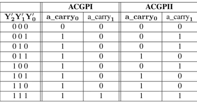
1.4.1.3 Accuracy-Configurable Approximate Adder . . . 50
1.4.1.4 Gracefully-Degrading Adder . . . 55
1.4.1.5 Addition Using Approximate Full-Adder Logic . . . 61
1.4.1.6 Approximate Adders by Probabilistic Pruning of Existing Designs . . . 65
1.4.2 Approximate Integer Multiplication . . . 67
1.4.2.1 Approximate Array Multipliers . . . 68
1.4.2.2 Error-Tolerant Multiplier . . . 74
1.4.2.3 Approximate Multipliers using Modified Booth Encoding . . 77
1.4.2.4 Dynamic Range Unbiased Multiplier . . . 87
1.4.3 Final Discussion on Approximate Operators in Literature . . . 90
2 Leveraging Power Spectral Density in Fixed-Point System Refine-ment 93 2.1 Motivation for Using Fixed-Point Arithmetic in Low-Power Computing . . . . 93
2.2 Related work on accuracy analysis . . . 94
2.3 PSD-based accuracy evaluation . . . 98
2.3.1 PSD of a quantization noise . . . 98
2.3.2 PSD propagation across a fixed-point Linear and Time-Invariant (LTI) system . . . 99
2.4 Experimental Results of Proposed Power Spectral Density (PSD) Propagation Method . . . 100
2.4.1 Experimental Setup . . . 101
2.4.1.1 Finite Impulse Response (FIR) and Infinite Impulse Response (IIR) Filters . . . 101
2.4.1.2 Frequency Domain Filtering . . . 101
2.4.1.3 Daubechies 9/7 Discrete Wavelet Transform . . . 101
2.4.2 Validation of the Approach for LTI Systems . . . 103
2.4.3 Influence of the Number of PSD Samples . . . 103
2.4.4 Comparison with PSD-Agnostic Methods . . . 104
2.4.5 Frequency Repartition of Output Error . . . 105
2.5 Conclusions about PSD Estimation Method . . . 106
3 Fast Approximate Arithmetic Operator Error Modeling 107 3.1 The Problem of Analytical Methods for Approximate Arithmetic . . . 107
3.2 Bitwise-Error Rate Propagation Method . . . 109
3.2.1 Main Principle of Bitwise-Error Rate (BWER) Propagation Method . . 109
3.2.2 Storage Optimization and Training of the BWER Propagation Data Structure . . . 110
3.2.3 BWER Propagation Algorithm . . . 112
3.3 Results of the BWER Method on Approximate Adders and Multipliers . . . 113
3.3.1 BWER Training Convergence Speed . . . 114
3.3.2 Evaluation of the Accuracy of BWER Propagation Method . . . 114
3.3.3 Estimation and Simulation Time . . . 119
3.3.4 Conclusion and Perspectives . . . 120
3.4 Modeling the Effects of Voltage Over-Scaling (Voltage OverScaling (VOS)) in Arithmetic Operators . . . 122
3.4.1 Characterization of Arithmetic Operators . . . 123
3.4.2 Modelling of VOS Arithmetic Operators . . . 124
3.4.3 Conclusion . . . 130
4 Approximate Operators Versus Careful Data Sizing 133 4.1 ApxPerf: Hardware Performance and Accuracy Characterization Framework for Approximate Computing . . . 133
4.1.1 ApxPerf– First Version . . . 134
4.1.2 ApxPerf– Second Version . . . 136
4.2 Raw Comparison of Fixed-Point and Approximate Operators . . . 140
4.3 Comparison of Fixed-Point and Approximate Operators on Signal Processing Applications . . . 144
4.3.1 Fast Fourier Transform . . . 144
4.3.2 JPEG Encoding . . . 144
4.3.3 Motion Compensation Filter for HEVC Decoder . . . 146
4.3.4 K-means Clustering . . . 148
4.4 Considerations About Arithmetic Operator-Level Approximate Computing . . 149
5 Fixed-Point Versus Custom Floating-Point Representation in Low-Energy Computing 151 5.1 ct_float: a Custom Synthesizable Floating-Point Library . . . 151
5.1.1 Thect_float Library . . . 152
5.1.2 Performance ofct_float Compared to Other Custom Floating-Point Libraries . . . 155
5.2 Stand-Alone Comparison of Fixed-Point and Custom Floating-Point . . . 161
5.3 Application-Based Comparison of Fixed-Point and Custom Floating-Point . . . 163
5.3.1 Comparison on K-Means Clustering Application . . . 164
5.3.1.1 K-Means Clustering Principle, Algorithm and Experimental Setup . . . 164
5.3.1.2 Experimental Results on K-Means Clustering . . . 167
5.3.2 Comparative Results on Fast Fourier Transform Application . . . 168
5.4 FxP vs FlP – Conclusion and Discussion . . . 171
Acronyms 181
Publications 183
Bibliography 190
List of Figures 191
Introduction
Handling The End Of Moore’s Law
In the History of computers, huge improvements in calculation accuracy have been made in two ways. First, the accuracy of computations was gradually improved with the increase of the bit width allocated to number representation. This was made possible thanks to technology evolution and miniaturization, allowing a dramatical growth of the number of basic logic el-ements embedded in circuits. Second, accurate number representations such as floating-point were proposed. Floating-point representation was first used in 1914 in an electro-mechanical version of Charles Babbage’s computing machine made by Leonardo Torres y Quevedo, the Analytical Engine, followed by Konrad Zuse’s first programmable mechanical computer em-bedding 24-bit floating-point representation. Today, silicon-based general-purpose processors mostly embed 64-bit floating-point computation units, which is nowadays standard in terms of high-accuracy computing.
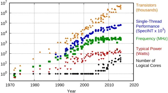
At the same time, important improvements of computational performance have been per-formed. The miniaturization, besides allowing larger bit-width, also allowed considerable ben-efits in terms of power and speed, and thus energy. CDC 6600 supercomputer created in 1964, with its 64K 60-bit words of memory, had a power consumption of approximatively 150 kW for a computing capacity of approximatively 500 KFLOPS, which makes 3.3 floating-point operations per Watt. In comparison, best 2017’s world’ supercomputer Sunway TaihuLight in China with its 1.31 Pbytes of memory, announces 6.05 GFLOPS/W [5]. Therefore, in forty years, the supercomputers energy efficiency has improved by roughly2E9, following the needs of industry. These impressive progresses were achieved according to Moore’s law, who fore-cast in 1965 [6] an exponential growth of computation circuit complexity, depicted in Figure 1 in terms of transistor count, performance, frequency, power and number of processing cores. From the day it was stated, this law and its numerous variations have outstandingly described the evolution of computing, but also the needs of the global market, such as computing is now inherent to nearly all possible domains, from weather forecasting to secured money transac-tions, including targeted advertising and self-driving cars.
However, many specialists agree on Moore’s Law to end in a very near future [7]. First of all, the gradual decrease of the size of silicon transistors is coming to an end. With a Van Der Waals radium of 210 pm, today’s 10 nm transistors are less than 50 atoms large, leading new issues at quantum physics scale, as well as increased current leakage. Then, the 20th century has known a steady increase of clock frequency in synchronous circuit, which represent the overwhelming majority of circuits, helping the important gain in performance. However, the
100 101 102 103 104 105 106 107 1970 1980 1990 2000 2010 2020 Number of Logical Cores Frequency (MHz) Single-Thread Performance (SpecINT x 103) Transistors (thousands) Typical Power (Watts) Year
Figure 1 – 45 years of microprocessor trend data, collected by M. Horowitz, F. Labonte, O. Shacham, K. Olukotun, L. Hammond, and C. Batten and completed by K. Rupp
beginning of the third millennium has seen a stagnation of this frequency, enforcing perfor-mance to be found in parallelism instead, single-core disappearing in favor of multi/many-core processors.
Technology being pushed to its limits and a new cutting-edge physical-layer technology not appearing to arrive soon, new ways have to be found for computing to follow the needs. Moreover, with a strong interest of industry into critical embedded systems, energy-efficiency is sought more than ever. Specialists are anticipating a future technological revolution brought by the Internet Of Things (IOT), with a fast growth of the number of interconnected au-tonomous embedded systems [8, 9, 10]. As said above, a first performance improvement can be found in computing parallelism, thanks to multi-core/multi-thread superscalar or VLIW proces-sors [11], or GPU computing. However, not all applications can be well parallelized because of data dependencies, leading to moderate speed-up in spite of an important area and energy over-head. A second modern way to improve performance is the use of hardware accelerators. These accelerators come in mainstream processors, with hardware video encoders/decoders such as for x264 or x265 codecs, but also in Field-Programmable Gate Arrays (FPGAs). FPGAs con-sist in a grid of programmable logic gates, allowing reconfigurable hardware implementation. In addition of general-purpose Look-Up Tables (LUTs), most FPGAs embed Digital Signal Processing blockss (DSPs) to accelerate signal processing computations. Hybrids embedding processors connected to an FPGA, embodied by Xilinx Zynq family, are today a big stake for high-performance embedded systems. Nevertheless, hardware and software co-design still represents an important cost in terms of development and testing.
Approximate Computing or Playing with Accuracy for Energy
Effi-ciency
This thesis focuses on an alternative way to improve performance/energy ratio, which is re-laxing computation accuracy to improve performance, as well in terms of energy/area for low-power systems, but also in terms of speed for High Performance Computing (HPC). Indeed, for many reasons, many applications can tolerate some imprecision for various reasons. For instance, having a high accuracy in signal processing applications can be useless if the input signals are noisy, since the least significant bits in the computation will be only applied on the noisy part of the signal. Also, some applications such as classification do not always have golden output and can tolerate a set of satisfying results. Therefore, it is useless to perform many loop iterations to get an output which can be considered as good enough.
Various methods applied at several levels are possible to relax the accuracy to get per-formance or energy benefits. At physical layer, voltage and frequency can be scaled beyond the circuit tolerance threshold with potential important energy of speed benefits, but with ef-fects on the quality of the output that may be destructive and hard to be managed [12, 13]. At algorithmic level, several simplifications can be performed such as loop perforation or mathe-matical functions approximations. For instance, trigonometric functions can be approximated using COordinate Rotation DIgital Computing (CORDIC) [14] with limited number of itera-tions, and complex functions can be approximated by interval using simple polynomials stored in small tables. The choice and management of arithmetic paradigms also allows important energy savings while relaxing accuracy.
In this thesis, three main paradigms are explored: • customizing floating-point operators,
• reducing bit-width and complexity using fixed-point arithmetic, which can be associated to quantization theory,
• and approximate integer operators, which perform arithmetic operations using inaccurate functions.
Floating-point arithmetic is often associated to high-precision computing with important time and energy overhead compared to fixed-point. Indeed, floating-point is today the most used representation of real numbers because of its high dynamic and high precision at any amplitude scale. However, because of more complex operations than for integer arithmetic and the complexity of the many particular cases handled in IEEE 754 standard [15], fixed-point is nearly always selected when low energy per operation is aimed at. In this thesis, we consider simplified small-bitwidth floating-point arithmetic implementations leading to better energy efficiency.
Fixed-point arithmetic is the most classical paradigm when it comes to low-energy comput-ing. In this thesis, it is used as a reference for comparisons with the other paradigms. A model for fixed-point error estimation leveraging Power Spectral Density (PSD) is also proposed.
Finally, approximate arithmetic operators using modified addition and multiplication func-tions are considered. Many implementafunc-tions of these operators were published this past decade, but they have never been the object of a complete comparative study.
After presenting literature about floating-point and fixed-point, a study of state-of-the-art approximate operators is proposed. Then, models for error propagation for fixed-point and ap-proximate operators are described and evaluated. Finally, comparative studies between approx-imate operators and fixed-point on one side, and fixed-point and floating-point on the other side, leveraging classical signal processing applications. More details on the organization of this document are given in the next section.
Thesis Organization
Chapter 1 Approximate computing in general is presented, followed by a deeper study on the different existing computing arithmetic. After a presentation of classical floating-point and fixed-point arithmetic paradigms, state-of-the-art integer approximate adders and multipliers are presented to give an overview of the many existing techniques to lower energy introducing inaccuracy in computations.
Chapter 2 A novel technique to estimate the impact of quantization across large fixed-point systems is presented, leveraging the noise Power Spectral Density (PSD). The benefits of the method compared to others is then demonstrated on signal processing applications.
Chapter 3 A novel technique to estimate the error of integer approximate operators error propagated across a system is presented in thus chapter. This technique, based on Bitwise Error-Rate (BWER), first uses training by simulation to build a model, which is then used for fast propagation. This analytical technique is fast and requires less space in memory than other similar existing techniques. Then, a model for the reproduction of Voltage Over-Scaling (VOS) error in exact integer arithmetic operators using pseudo-simulation on approximate operators is presented.
Chapter 4 A comparative study of fixed-point and approximate arithmetic is presented in Chapter 4. Both paradigms are first compared in their stand-alone version, and then on several signal processing applications using relevant metrics. The study is performed using the first version of our open-source operator characterization framework ApxPerf, and our approximate operator libraryapx_fixed.
Chapter 5 Using a second version of our frameworkApxPerf embedding a High Level Synthesis (HLS) frontend and our custom floating-point library ct_float, a comparative study of fixed-point and small-width custom floating-point arithmetic is performed. First, the hardware performance and accuracy of both operators are compared in their stand-alone ver-sion. Then, this comparison is achieved in K-means clustering and Fast Fourier Transform (FFT) applications.
Trading Accuracy for Performance in
Computing Systems
In this Chapter, various methods to trade accuracy for performance are first listed in Section 1.1. Then, the study is centered on the different existing representations of numbers and the archi-tectures of the arithmetic operators using them. In Section 1.2, floating-point arithmetic is de-veloped. Then, Section 1.3 presents fixed-point arithmetic. Finally, a study of state-of-the-art approximate architectures of integer adders and multipliers is presented in Section 1.4.
1.1 Various Methods to Trade Accuracy for Performance
In this section, the main methods to trade accuracy for performance are presented. First, VOS is discussed. Then, existing algorithm-level transformations are presented. Finally, approximate arithmetic is introduced, to be further developed in Sections 1.2, 1.3, and 1.4 as the central element of this thesis.
1.1.1 Voltage Overscaling
The power consumption of a transistor in a synchronous circuit is linear with the frequency and proportional to the square of the voltage applied. For a same load of computations, decreasing frequency also increases computing time and the energy is the same. Thus, it is important to mostly exploit the voltage to save as much energy as possible. Nevertheless, decreasing voltage implies more instability in the transitions of the transistor, and this is why in a large majority of systems, the voltage is set above a certain threshold which ensures the stability of the system. Lowering the voltage under this threshold can cause the output of the transistor to be stuck to 0 or 1, compromising the integrity of the realized function.
One of the main issues of VOS is process variability. Indeed, two instances A and B of a same silicon-based chip are not able to handle the exact same voltage before breakdown, a given transistor in A being possibly weaker than the same in B, mostly because of Random Dopant Fluctuations (RDF) which are a major issue in nanometer-scale Very Large Scale Integration (VLSI). However, with the important possible energy gains brought by VOS, its mastering is
an important stake which is widely explored [12, 13]. Low-leakage technologies like Fully Depleted Silicon On Insulator (FDSOI) allow RDF to impact much less near-threshold puting variability. Despite technology improvements, near-threshold and sub-threshold com-puting needs error-correcting circuits, coming with an area, energy and delay overhead which needs to be inferior to the savings. In [16], a method called Razor is proposed to monitor at low cost circuit error rate to tune its voltage to get an acceptable failure rate. Therefore, the main challenge with VOS is its uncertainty, the absence of a general rule which would make all instances of an electronic chips equal towards voltage scaling, which make manufacturers generally turn their backs to VOS, preferring to keep a comfortable margin above the threshold. In next Subsections 1.1.2 and 1.1.3, accuracy is traded for performance in a reproducible way, with results which are independent from hardware and totally dependent from the pro-grammer/designer’s will, and thus more likely to be used in the future at industrial scale.
1.1.2 Algorithmic Approximations
A more secure way than VOS to save energy is achieved by algorithmic approximations. In-deed, modifying algorithm implementation to make them deliver their results in less cycles or using less intensively costly functions potentially leads to important savings. First, the approx-imable parts of the code or algorithm must be identified, i.e. the parts where the gains can be maximized despite a moderate impact on the output quality. Various methods for the identi-fication of these approximable parts are proposed in [17, 18, 19]. These methods are mostly perturbation-based, meaning errors are inserted in the code, and the output is simulated to evaluate the impact of the inserted error. As all simulation-based methods, these methods may not be scalable to large algorithms and only consider a limited number of perturbation types. Once the approximable parts identified by an automatized method or manually, depending on the kind of algorithm part to approximate (computation loops, mathematical functions, etc), different techniques can be applied.
One of the main techniques for reducing the cost of algorithm computations is loop perfo-ration. Indeed, most signal processing algorithms consist in quite simple functions repeated a high number of times, e.g. for Monte Carlo simulations, search space enumeration or iterative refinement. In these three cases, a subset of loop iterations can simply be skipped, yet returning good enough results [20]. Using complex mathematical functions such as exponentials, loga-rithms, square roots or trigonometric functions is very area, time and energy-costly compared to basic arithmetic operations. Indeed, accurate implementations may require large tables and long addition and multiplication-based iterative refinement. Therefore, in applications using intensively these mathematical functions, releasing accuracy for performance can be source of important savings. A first classical way to approximate functions is polynomial approxima-tion, using tabulated polynomials representing the function in different ranges. In the context of approximate computing, iterative-refinement based mathematical approximations are also very interesting since they allow loop perforation discussed previously. Reducing the number of iterations can be applied to CORDIC algorithms, very common for trigonometric function approximations [14]. Several efficient approximate mathematical functions were proposed for specialized hardware such as FPGAs [21] or Single Instruction Multiple Data (SIMD)
hard-ware [22].
1.1.3 Approximate Basic Arithmetic
The level of approximation we focus on in this thesis is the approximation of basic arithmetic operations, which are addition, subtraction and multiplication. These operations are the base for most functions and algorithms in classical computing, but also the most energy-costly com-pared to other basic CPU functions such as register shifts or binary logical operators, meaning that a gain in performance or energy on these operations automatically induces an important benefit for the whole application. They are also statistically intensively used in general-purpose CPU computing: in ARM processors,ADD and SUB instructions are the instructions the most
used afterLOAD and STORE. The approximation of these basic operators is explored along
two different angles in this thesis. On the one hand, approximate representations of numbers is discussed, more precisely the approximate representation of real numbers in computer arith-metics, using floating-point and fixed-point arithmetic. On the other hand, approximate com-puting using modified functions for integer arithmetical functions of addition, subtraction and multiplication is explored used in fixed-point arithmetic and compared to existing methods.
Approximations using floating-point arithmetic are discussed in Section 1.2, approxima-tions using fixed-point arithmetic in Section 1.3 and approximate integer operators are pre-sented in Section 1.4.
1.2 Relaxing Accuracy Using Floating-Point Arithmetic
Floating-point (Floating-Point (FlP)) representation is today the main representation for real numbers in computing, thanks to a potentially high dynamic, totally managed by the hardware. However, this ease of use comes with relatively important area, delay and energy penalties. FlP representation is presented in Section 1.2.1. Then, FlP addition/subtraction and multiplication are described in Section 1.2.2. Ways to relax accuracy for performance in FlP arithmetic is then discussed in Section 1.2.3.
1.2.1 Floating-Point Representation for Real Numbers
In computer arithmetic, the representation of real numbers is a major stake. Indeed, most pow-erful algorithms are based on continuous mathematics, and their accuracy and stability is di-rectly related to the accuracy of the number representation they use. However, in classical computing, an infinite accuracy is not possible since all representations are contained in a fi-nite bit width. To address this issue, having a number representation as accurate for very small numbers and very large numbers is important. Indeed, large and small numbers are dual, since multiplying (resp. dividing) a number by another large number is equivalent to dividing (resp. multiplying) by a small number. Giving the same relative accuracy to numbers whatever their amplitude is can only be achieved giving the same impact to their most significant digit. In decimal representation, this is achieved with scientific notation, representing the significant
value of the number in the range[1, 10[, weighted by 10 elevated to a certain power. FlP rep-resentation in radix-2 is the pendant of the scientific notation for binary computing. The point in the representation of the number is "floating" so the representative value of the number (or
mantissa) represents a number in [1, 2[, multiplied by a power of 2. Given an M-bit mantissa,
a signed integer exponent of value e, often represented in biased representation, and a sign bit
s, any real number between limits defined by M and E the number of bits allocated to the
exponent e can be represented with a relative step depending on M by: (≠1)s
◊ mM≠1.mM≠2mM≠3· · · m1m0◊ 2e.
With this representation, any number under this format can be represented using M+E+1 bits as showed in Figure 1.1. A particularity of binary FlP with a mantissa represented in[1, 2[ is that its Most Significant Bit (MSB) can only be1. Knowing that, the MSB can be left implicit, freeing space for one more Least Significant Bit (LSB) instead.
𝑒3 𝑒2 𝑒1 𝑒0 𝑚5 𝑚4 𝑚3
Exponent Mantissa
Sign
𝑚6 𝑚2 𝑚1 𝑚0
𝑠
Figure 1.1 – 12-bit floating-point number with 4 bits of exponent and 7 bits of mantissa Nevertheless, automatically keeping the floating point at the right position along
compu-tations requires an important hardware overhead, as discussed in Section 1.2.2. Managing sub-normal numbers (numbers between0 and the smallest positive possible representable value), the values 0 and infinity also represent an overhead. Despite this additional cost, FlP represen-tation is today established as the standard for real number represenrepresen-tation. Indeed, besides its high accuracy and high dynamic, it has the huge advantage of leaving the whole management of the representation to the hardware instead of leaving it to the software designer, significantly diminishing developing and testing time. This domination is sustained by IEEE 754 standard, last revised in 2008 [15], which sets the conventions for floating-point number possible repre-sentation, subnormal numbers management and the different cases to be handled, ensuring a high portability of programs. However, such a strict normalization implies:
• an important overhead for throwing flags for the many special cases, and even more important overhead for the management of these special cases (hardware or software overhead),
• and a low flexibility in the width of the mantissa and exponent, which have to respect the rules of Table 1.1 for 32, 64 and 128-bit implementation.
As a first conclusion, the constraints imposed to FlP representation by IEEE 754 normaliza-tion imply a high cost in terms of hardware resource, which highly counterbalance its accuracy benefits. However, as discussed in Section 1.2.3, taking liberties with FlP can significantly increase the accuracy/cost ratio.
Precision Mantissa Exponent Max decimal Exponentwidth width exponent bias
Single precision 24 8 38.23 127
Double precision 53 11 307.95 1023
Quadruple precision 113 15 4931.77 16383
Table 1.1 – IEEE 754 normalized floating-point representation
1.2.2 Floating-Point Addition/Subtraction and Multiplication
As discussed later in Section 1.3, integer addition/subtraction is the simplest arithmetic opera-tor. However, in FlP arithmetic, it suffers from a high control overhead. Indeed, several steps are needed to perform the FlP addition:
• First, the difference of the exponents is computed.
• If the difference of the exponents is superior to the mantissa width, the biggest number is directly issued (this is thefar path of the operator – one of the numbers is too small
to impact the addition).
• Else, if the difference of the exponents is inferior to the mantissa width, one of the inputs’ mantissas must be shifted so bits of same significance are facing each other. This is the
close path, by opposition with the far path.
• The addition of the mantissas is performed.
• Then, rounding is performed on the mantissa, depending on the dropped bits and the rounding mode selected.
• Special cases are then handled (zero, infinity, subnormal results), and the output sign. • Then, mantissa is shifted so it represents a value in [1, 2[, and the exponent is modified
depending on the number of shifts.
FlP addition principle is illustrated in Figure 1.2 taken from [23]. More control can be needed, depending on the implementation of the FlP adder and the specificities of the FlP represen-tation. For instance, management of the implicit 1 implies to add 1s to the mantissas before addition, and an important overhead can be dedicated to exception handling.
For cost comparison, Table 1.2 shows the performance of 32-bit and 64-bit FlP addition, usingac_float type from Mentor Graphics, and 32-bit and 64-bit integer addition using ac_int
type, generated using the HLS and power estimation process of the second version of Apx-Perf framework described in Section 4.1, targeting 28nm FDSOI with a 200 MHz clock and using 10, 000 uniform input samples. FlP addition power was estimated activating the close path50% of the time. These results show clearly the overhead of FlP addition. For 32-bit ver-sion, FlP addition is3.5◊ larger, 2.3◊ slower and costs 27◊ more energy than integer addition. For 64-bit version, FlP addition is3.9◊ larger, 1.9◊ slower and costs 30◊ more energy. The
LZC/shift p + 1 p + 1 p + 1 2p + 2 p p p + 1 p p + 1 x y z
exp. difference / swap
rounding,normalization and exception handling
mx ex c/f +/– ex ey
close path
c/f ex ez my shift |mx my| my 1-bit shift ex ez mxfar path
stickyprenorm (2-bit shift)
s s0 s0= 0 g r mz mz
Figure 1.2 – Dual-path floating-point adder [23]
Area Total Critical Power-Delay (µm2) power (mW) path (ns) Product (fJ)
32-bit 653 4.39E≠4 2.42 1.06E≠3
ac_float
64-bit 1453 1.12E≠3 4.02 4.50E≠3
ac_float
32-bit 189 3.66E≠5 1.06 3.88E≠5
ac_int
64-bit 373 7.14E≠5 2.10 1.50E≠4
ac_int
overhead seems to be roughly linear with the size of the operator, and the impact of numbers representation is highly impacting the performance. However, it is showed in Chapter 5 that this high difference shrinks when the impact of accuracy is taken into account.
FlP multiplication is less complicated than addition as only a low control overhead is neces-sary to perform the operation. Input mantissas are multiplied using a classical integer multiplier (see Section 1.3), while exponents are simply added. At worse, a final+1 on the exponent can be needed, depending on the result of the mantissas multiplication. The basic architecture of a FlP multiplier is described in Figure 1.3 from [23]. Obviously, all classical hardware
over-1 0 0 1 incrementer p p p 1 p 1 2p z 1 or mz inc mode rounding logic b 1 b ez+ b ey+ b 1.mx 1.my ex+ b z 1· · · z p+1 z 1z0z1· · · z2p 2 z p s z0· · · zp 2 e x + e y + b e x + e y + b +1 z p 1 zp+1· · · z2p 2 c out sticky
Figure 1.3 – Basic floating-point multiplication [23]
heads needed by FlP representation are necessary (rounding logic, normalization, management of particular cases). Table 1.3 shows the difference between 32-bit and 64-bit floating-point multiplication using Mentor Graphicsac_float and 32-bit and 64-bit fixed-width1integer mul-tiplication usingac_int data type, with the same experimental setup than discussed before for
the addition.
A first observation on the area shows that the integer multiplication is 48% larger than FlP version for 32-bit version, and37% larger for 64-bit version. This difference is due to the smaller size of the integer multiplier in the FlP multiplication, since it is limited to the size of the mantissa (24 bits for 32-bit version, 53 bits for 64-bit version). Despite the management of the exponent, the overhead is not large enough to produce a larger operator. However, if the overhead area is not very large, 32-bit FlP multiplication energy is11◊ higher than the integer multiplication energy, while 64-bit version is37◊ more energy-costly. It is interesting to note that the difference of energy consumption between addition and multiplication is much more important for integer operators than for FlP. For 32-bit version for instance, integer multiplica-1An operator is considered as fixed-width when its output has the same width as its inputs. In the considered
Area Total Critical Power-Delay (µm2) power (mW) path (ns) Product (fJ)
32-bit 1543 8.94E≠4 2.09 1.87E≠3
ac_float
64-bit 6464 6.56E≠3 4.70 3.08E≠2
ac_float
32-bit 2289
6.53E≠5 2.38 1.55E≠4
ac_int
64-bit 8841 1.84E≠4 4.52 8.31E≠4
ac_int
Table 1.3 – Cost of floating-point multiplication vs integer multiplication
tion consumes4.7◊ more energy than integer addition, while this factor is only 1.4◊ for 32-bit FlP multiplier compared to 32-bit FlP adder. Therefore, using multiplication in FlP computing is relatively less penalizing than for integer multiplication, typically used in Fixed-Point (FxP) arithmetic.
1.2.3 Potential for Relaxing Accuracy in Floating-Point Arithmetic
There are several possible opportunities to relax accuracy in floating-point arithmetic to in-crease performance. The main one is simply to use word-length as small as possible for the mantissa and the exponent. With normalized mantissa in[1, 2[, reducing the word-length cor-responds to pruning the LSBs, which comes with no overhead. Eventually, rounding can be performed at higher cost. For the exponent, the transformation is more complicated if it is rep-resented with a bias. Indeed, if e is the exponent width, an implicit bias of2e≠ 1 applies to
the exponent in classical exponent representation. Therefore, reducing the exponent to a width
eÕmeans that a new bias must be applied. The original exponent must be added2eÕ≠ 2e(< 0)
before pruning MSBs, implying hardware overhead at conversion. The original exponent must represent a value inË≠2eÕ≠1+ 1, 2eÕ≠1Èto avoid overflow. In practice, it is better to keep a con-stant exponent width to avoid useless overhead and conversion overflows which would have a huge impact on the quality of the computations, even if they are scarce.
A second way to improve computation at inferior cost is to play with the implicit bias of the exponent. Indeed, increasing the exponent width increases the dynamic towards infinity, but also the accuracy towards zero. Thus, if the absolute maximum values to be represented are known, the bias can be chosen so it is just large enough to represent these values. This way, the exponent gives more accuracy to very small values, increasing accuracy. However, using a custom bias means that the arithmetical operators (addition and multiplication) must consider this bias in the computation of resulting exponent, and the optimal bias along computation may diverge to ≠Œ. To avoid this, if the original 2e≠ 1 exponent bias is kept, exponent bias can be
simulated by biasing the exponents of the inputs of each or some computations using shifting. For the addition, biasing both inputs adding 2ein to the exponent implies that the output will also be represented biased by2ein. For the multiplication, the output will be biased by2ein+1.
Keeping an implicit track of the bias along computations allows to know any algorithm output bias, and eventually to perform a final rescaling of the outputs.
Finally, accuracy can be relaxed in the integer operators composing FlP operators, i.e. the integer adder adding mantissas in FlP addition close path, and the integer multiplier in the FlP multiplication. Indeed, they can be replaced by the approximated adders and multipliers described in Section 1.4 to improve performance relaxing accuracy. However, as the most part of the performance cost is in control hardware more than in integer arithmetic part, the impact on accuracy would be strong for a very small performance benefit. The same approximation can be applied on exponent management, but the impact of approximate arithmetic would be huge on the accuracy and is strongly unadvised.
More state-of-the-art work on FlP arithmetic is developed in Section 5.1, more particularly on HLS using FlP custom computing cores.
1.3 Relaxing Accuracy Using Fixed-Point Arithmetic
Aside from FlP, a classical representation for real numbers is Fixed-Point (FxP) representation. This Section presents generalities about FxP representation in Section 1.3.1, then presents the classical models for quantization noise in Section 1.3.2. Finally, hardware implementations of addition and multiplication are respectively listed and discussed in Sections 1.3.3 and 1.3.4.
1.3.1 Fixed-Point Representation for Real Numbers
In fixed-point representation, an integer number represents a real number multiplied by a fac-tor depending on the implicit position of the point in the representation. A real number x is represented by the FxP number xFxPrepresented on n bits with d bits of fractional part by the following equation:
xFxP=
--x◊ 2d---r◊ 2≠d,
where |·|ris a rounding operator, which can be implemented using several functions such as
the ones of Section 1.3.2. The representation of a 12-bit two’s complement signed FxP number with a 4-bit integer part is depicted in Figure 1.4.
𝑥11 𝑥10 𝑥9 𝑥8 𝑥7 𝑥6 𝑥5 𝑥4 𝑥3
22 21 20 2−1 2−2 2−3 2−4 2−5
Integer part Fractional part
−23
𝑥2 𝑥1 𝑥0
2−7 2−8
2−6
Figure 1.4 – 12-bit fixed-point number with 4 bits of integer part and 8 bits of fractional part In two’s complement representation, the MSB has a negative weight, such as a binary
number xbin= {xi}iœ[0,n≠1]represents the integer number xintthe following way: xint = xn≠1◊ 1 ≠2n≠12+ nÿ≠2 i=0 xi◊ 2i
Therefore, the two’s complement n-bit FxP number represented by xFxPwith d-bit fractional part is worth: xFxP= xint◊ 2≠d = xn≠1◊ 1 ≠2n≠d≠12+ nÿ≠2 i=0 xi◊ 2i≠d.
1.3.2 Quantization and Rounding
Representing a real number in FxP is equivalent to transforming a number represented on an infinity of bits to a finite word-length. This reduction is generally referred asquantization of a continuous amplitude signal. Using a FxP representation with a d-bit fractional part implies
that the step between two representable values is equal to q = 2≠d, referred asquantization
step. The process of quantization results in a quantization error defined by:
e= xq≠ x, (1.1)
where x is the original number to be quantified and xqthe resulting quantified number.
Quantization of continuous amplitude signal is performed differently depending on the rounding mode chosen. Several classical rounding modes are possible:
1. Rounding towards ≠Œ (RD). The infinity of bits dropped are not taken into considera-tion. This results in a negative quantization error e and is equivalent to truncaconsidera-tion. 2. Rounding towards+Œ (RU). Again, the infinity of bits dropped are not taken into
con-sideration, and the nearest superior representable value is selected. This is equivalent to adding q to the result of the truncation process.
3. Rounding towards 0 (RZ). If x is negative, the number is rounded to +Œ. Else, it is rounded to ≠Œ
4. Rounding to Nearest (RN). The nearest representable value is selected – if the MSB of the dropped bits is0, then xq is obtained by rounding to ≠Œ (truncation) – else xq is
obtained by rounding towards+Œ. The special value where the MSB of the dropped part is1 and all the following bits are 0 can lead whether to rounding up or down depending on the implementation. Choosing one or another case does not change anything in the error distribution in the case of continuous amplitude signal, which is also the case for discrete case, as said below.
(a) Quantization error distribution for rounding to-wards ≠Œ
(b) Quantization error distribution for rounding to-wards+Œ
(c) Quantization error distribution for rounding to nearest
Figure 1.5 – Distribution of continuous signal quantization error for rounding towards ±Œ and rounding to nearest
The quantization error produced by rounding towards ±Œ and to nearest discussed above are depicted in Figure 1.5. RZ method has a varying quantization error distribution depending on the sign of the value to be rounded. As described in [24] and [25], the additional error due to the quantization of a continuous signal is uniformly distributed between its limits ([≠q, 0] for truncation,[0, q] for rounding towards +Œ and [≠q/2, q/2] for rounding to nearest) and statistically independent on the quantized signal. Therefore, the mean and variance of the error are perfectly known in these cases and are indexed in Table 1.4. Thanks to its independence to the signal, quantization error can be seen as an additive uniformly distributed white noise
q such as depicted in Figure 1.6. This representation of quantization error is the base of FxP
representation error analysis discussed in the next Chapter.
Figure 1.6 – Representation of FxP quantization error as an additive noise
The previous paragraphs describe the properties of the quantization of a continuous signal. However, in FxP arithmetic, it is necessary to reduce the bit width along computations to avoid a substantial growth of the necessary resources. Indeed, as discussed in Section 1.3.4, an integer
multiplication needs to produce an output which width is equal to the sum of its inputs to get a perfectly accurate computation. However, the LSBs of the result are often not significant enough to be kept, and so a reduction of data width must be performed to save area, energy and time. Therefore, it is often necessary to reduce a FxP number x1 with d1-bit fractional part to another FxP number x2 with d2-bit fractional part, where d2 < d1. This reduction leads to a discrete quantization error distribution, depending on the number of bits dropped db= d1≠d2.
This distribution is still uniform for RD, RU and RN rounding methods, but has a different bias. Moreover, for RN method, this bias is not 0, and depends on the direction of rounding chosen when the MSB of the dropped part is1 and all the other dropped bits 0. This can lead to divergences when accumulating a large number of computations.
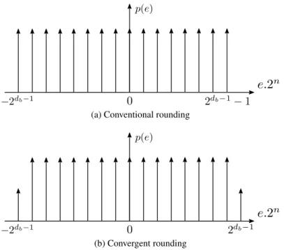
(a) Conventional rounding
(b) Convergent rounding
Figure 1.7 – Comparison of quantization error distribution of conventional rounding and con-vergent rounding
To overcome this possible deviation, Convergent Rounding to Nearest (CRN) was pro-posed in [26]. When the special case cited above is met, the rounding is once performed toward +Œ, and once towards ≠Œ. This way, the quantization error distribution gets centered to zero. Figure 1.7 shows the effect of CRN on the error distribution compared to simpler RN. On Fig-ure 1.7a, the discrete uniform distribution of RN method has a negative bias of q
2
1
2≠db2. As
the highest error occurs for the specialin between case, distributing this error using
alterna-tively RD and RU paradigms balances the error, lowering by half the highest negative error and moving its impact to a new spike removing the bias as showed on Figure 1.7b. However, this compensation slightly increases the variance of the quantization error.
are listed in Table 1.4. As a reminder, RZ method is mixing RD and RU, and thus the final distribution of error strongly depends on the distribution of the signal around0.
Continous Amplitude Discrete Amplitude
µe ‡2e µe ‡e2 RD ≠q2 12q2 ≠2q11 ≠ 2≠db2 q2 12 1 1 ≠ 2≠2db2 RU q 2 q 2 12 q2 1 1 ≠ 2≠db2 q2 12 1 1 ≠ 2≠2db2 RN 0 q2 12 q2 1 2≠db2 q2 12 1 1 ≠ 2≠2db2 CRN 0 q2 12 0 q 2 12 1 1 ≠ 2≠2db+12
Table 1.4 – Mean and variance of quantization error depending on the rounding method and type of signal
The implementation of rounding methods discussed above depend of two parameters. In-deed, when quantizing x1 with d1-bit fractional part to x2 with d2-bit fractional part, where
d2 < d1, only the following information is needed:
• the round bit, which is the value of the bit indexed by d1≠ d2≠ 1 of x1,
• and the sticky bit, which is a logical or applied to the bits {0, ..., d1≠ d2≠ 2} of x1. The extraction ofround and sticky bits is illustrated in Figure 1.8. The horizontal stripes in x1 correspond to theround bit, and the tilted stripes to the bits implied in the computation of thesticky bit. Here, both are worth 1, and the rounding logic outputs 1, which can correspond
to RU, RN, or CRN. The possible functions performed by the different rounding functions which can be implemented in rounding logic block of Figure 1.8 are listed in Table 1.5. It is important to notice that for RD method, the value of round and sticky bits have no influence on the rounding direction. For RN method, if the default rounding direction is towards+Πwhen round/sticky bits are1/0, then the value of the sticky bit does not influence the rounded result. If it is up, the sticky bit has to be considered. Therefore, some hardware simplifications can be performed for RD and RN (down case) methods, by just dropping the unused bits.
Figure 1.8 – Example of quantization and rounding of a10-bit fixed-point number to a 6-bit fixed-point number Round Sticky RD RU RN CRN bit bit 0 0 ≠ ≠ ≠ ≠ 0 1 ≠ + ≠ ≠
1 0 ≠ + or alwaysAlways ≠+ Alternatively≠ and +
1 1 ≠ + + +
1.3.3 Addition and Subtraction in Fixed-Point Representation
The addition/subtraction in FxP representation is much simpler than the one of FlP described in Section 1.2.2. Indeed, FxP arithmetic is entirely based on integer arithmetic. Adding two FxP numbers can be performed in 3 steps:
1. Aligning the points of the two numbers, shifting one of them (software style) or driving their bits to the right input in the integer adder (hardware design style).
2. Adding the inputs using an integer adder.
3. Quantizing the output using methods of Section 1.3.2.
In this section, we will consider the addition (respectively subtraction) of two signed FxP num-bers x and y with a total bit width of resp. nx and ny, a fractional part width of dx and dy and
an integer part width of mx= nx≠ dxand my = ny≠ dy. In the rest of this chapter, a nx-bit
FxP number x with mx-bit integer part will be noted x(nx, mx).
To avoid overflows or underflows, the output z(nz, mz) of the addition/subtraction of x and
ymust respect the following equation:
mz= max (mx, my) + 1. (1.2)
Moreover, an accurate addition/subtraction must also respect:
dz = max (dx, dy) . (1.3)
The final process for FxP addition of x(6, 2) and y(8, 3) returning z(9, 4) then quantized to
zq(6, 4) is depicted by Figure 1.9. For the subtraction x ≠ y, the classical way to operate is to
compute yÕ
= ≠y before performing the addition x + yÕ
. In two’s complement representation, this is equivalent to performing yÕ = y + 1, where y is the binary inverse of y. The inversion is fast and requires small circuit, and adding1 can be performed during the addition step of Figure 1.9 (after shifting) to avoid performing one more addition for the negation.
As a first conclusion about FxP addition/subtraction, the cost of the operation mostly de-pends on two parameters: the cost of shifting the input(s), and the efficiency of integer addition. From this point, we will focus on the integer addition, which represent the majority of this cost. The integer addition can be built from the composition of 1-bit additions, taking each three inputs – the input bits xi, yiand the input carry ciand returning two outputs – the output sum
bit si and the output carry ci+1. This function is realized by the Full Adder (FA) function of
Figure 1.10 which truth table is described in Table 1.6.
The simplest addition structure is the Ripple Carry Adder (RCA), built by the direct com-position of FAs. Each FA of rank i takes the input bits and the input carry of rank i. It returns the output bit of rank i and the output carry of rank i+ 1, which is connected to the following full adder, resulting in the structure of Figure 1.11. This is theoretically the smallest possible area for an addition, with a complexity of O(n). However, this small area is counterbalanced
Figure 1.9 – Fixed-point addition process of x(6, 2) and y(8, 3) returning z(9, 4) quantized to
zq(6, 4)
Figure 1.10 – One-bit addition function – Full adder (or compressor 3:2)
xi yi ci ci+1 si 0 0 0 0 0 0 0 1 0 1 0 1 0 0 1 0 1 1 1 0 1 0 0 0 1 1 0 1 1 0 1 1 0 1 0 1 1 1 1 1
Figure 1.11 – 8-bit Ripple Carry Adder (RCA)
by a high delay also in O(n), while the theoretical optimum is O (log n) [27]. Therefore, RCA is only implemented when area budget is critical.
A classical improvement issued from the RCA is the Carry-Select Adder (CSLA). The CSLA is composed of elements containing two parallel RCA structures, one taking0 as input carry and the other taking1. When the actual value of the input carry is known, the correct result is selected. This pre-computation (or prediction) of the possible output values increases speed, which can reach at best a complexity of O(Ôn) when the variable widths of the basic elements are optimal, while more than doubling the area compared to classical RCA. An 8-bit version of CSLA is depicted in Figure 1.12, with basic blocks of size 2-3-3 from LSB to MSB. Therefore, the resulting critical path is 3 FAs and 3 multiplexers 2-1, from input carry to output carry, instead of 8 FAs for RCA. It is important to note that CSLA structure can be applied to any addition structure such as the ones described below, and not only RCA, which can lead to better speed performance.
Figure 1.12 – 8-bit RCA-based Carry-Select Adder (CSLA) with 2-3-3 basic blocks As already stated, the longest path in the adder starts from the input carry (or the input LSBs) and ends at the output carry (or output MSB). Therefore, propagating the carry across the operator as fast as possible is a major stake as long as high speed is required. It can whether be done duplicating hardware like for CSLA, but it can also be achieved by prioritizing the carry propagation. In FA design, the output is computed together with the output carry. In
![Figure 1.43 – Error vs delay for an identical power consumption for GDA and AC2A [42]](https://thumb-eu.123doks.com/thumbv2/123doknet/11592330.298782/66.893.202.760.294.803/figure-error-delay-identical-power-consumption-gda-ac.webp)


![Figure 1.48 – Probabilistic pruning results for Kogge-Stone and Han-Carlson adders [45]](https://thumb-eu.123doks.com/thumbv2/123doknet/11592330.298782/72.893.174.789.265.593/figure-probabilistic-pruning-results-kogge-stone-carlson-adders.webp)