Two-Target Algorithms for Infinite-Armed Bandits with Bernoulli Rewards
Texte intégral
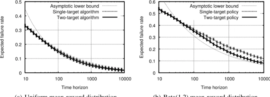
Figure
Documents relatifs
1: The Credit Assignment mecha- nism associates a reward to each operator, reflecting the operator impact on the progress of the search (e.g. fitness improvement); the
Two players, Ursule and Victor control this discrete dynamical system through their respective controls u and v, Ursule wants the system to reach the target.. Victor wants the system
Here we show that the randomization test is possible only for two-group design; comparing three groups requires a number of permutations so vast that even three groups
Symptoms Cholera = Shigella = acute watery acute bloody diarrhoea diarrhoea Stool > 3 loose > 3 loose.. stools per day, stools per day, watery like
L’archive ouverte pluridisciplinaire HAL, est destinée au dépôt et à la diffusion de documents scientifiques de niveau recherche, publiés ou non, émanant des
In order to serve them and gather generalizable knowledge at the same time, we formal- ize this situation as a multi-objective bandit problem, where a designer seeks to trade
Differential privacy of the Laplace mecha- nism (See Theorem 4 in (Dwork and Roth 2013)) For any real function g of the data, a mechanism adding Laplace noise with scale parameter β
