HAL Id: hal-01610999
https://hal.archives-ouvertes.fr/hal-01610999
Submitted on 28 Feb 2018
HAL is a multi-disciplinary open access
archive for the deposit and dissemination of
sci-entific research documents, whether they are
pub-lished or not. The documents may come from
teaching and research institutions in France or
abroad, or from public or private research centers.
L’archive ouverte pluridisciplinaire HAL, est
destinée au dépôt et à la diffusion de documents
scientifiques de niveau recherche, publiés ou non,
émanant des établissements d’enseignement et de
recherche français ou étrangers, des laboratoires
publics ou privés.
High heat flux mapping using infrared images processed
by inverse methods: An application to solar
concentrating systems
Victor Pozzobon, Sylvain Salvador
To cite this version:
Victor Pozzobon, Sylvain Salvador. High heat flux mapping using infrared images processed by inverse
methods: An application to solar concentrating systems. Solar Energy, Elsevier, 2015, 117, pp.29-35.
�10.1016/j.solener.2015.04.021�. �hal-01610999�
High heat flux mapping using infrared images processed by
inverse methods: An application to solar concentrating systems
Victor Pozzobon
⇑, Sylvain Salvador
Universite´ de Toulouse, Mines Albi, Centre RAPSODEE, UMR CNRS 5302, Campus Jarlard, route de Teillet, 81013 Albi CT Cedex 09, France
Abstract
With the spreading of solar concentrating devices and artificial suns, it has become critical to characterize the incident heat flux at the focal spot of such devices. In this paper a new method that allows the determination of incident heat flux at the focal spot concentrating devices has been developed. This approach is based on an inexpensive experimental device and basic inverse methods which are used to compute a map of the incident heat flux. The experimental setup is made of a common steel screen and an IR camera. Starting at ambient temperature, the screen is exposed to the incident heat flux. The evolution of the screen temperature field over time is recorded using the IR camera. The inverse model then uses temperature data to compute a map of the incident heat flux. Results at moderate heat flux were validated by comparison with Gardon radiometer readings: the agreement between the two methods is very good. This method yields a high resolution map without the need of an external scaling factor which is mandatory in the method using a CCD camera.
Keywords: Concentrating solar system; Heat flux mapping; Inverse methods
1. Introduction
Over the recent years interest in concentrated solar energy has grown. Indeed this source of power is able to achieve high heat flux and reach high temperatures. Thus it enables the study of high temperature (Guesdon et al.,
2006; Imhof, 1997) or high heating rate (Authier et al.,
2009) chemical processes, in order to better understand them. With time the use of solar concentrating devices has spread. Among them artificial suns are becoming more and more popular, as recently reviewed by Sarwar et al.
(2014). Indeed their power is available at will and their
operating parameters do not vary during the day.
A key problem with operating these devices is the knowledge of the heat flux distribution on the target sur-face. This problem has been approached using various methods. In some cases a radiometer (Llorente et al., 2011) or equivalent (Codd et al., 2010) is used to map the focal spot. Using this method is time consuming and offers a low spatial resolution map. Yet, it yields an absolute value of the incident heat flux and requires no external scal-ing factor. In other cases a CCD camera is used to record a grey value image of a water-cooled target (Sarwar et al.,
2014; Petrasch et al., 2007). Then using an external
mea-surement, often a radiometer reading, a scaling factor is applied to the recorded image. This method allows for a high resolution but relies entirely on the external scaling factor and the use of a high-end water-cooled target. One last way of mapping the heat flux distribution is to run the device at minimal power, for example using the moon
⇑Corresponding author.
instead of the sun as an outdoor dish (Kaushika and
Kaneff, 1987). Pictures can be taken and processed to yield
high resolution incident heat flux map. Then, the actual map can be computed using the ratio of the two source powers. Sadly, this is not possible for certain devices such as Xenon arc lamps because their minimal power is very close to their nominal operating condition.
Heat flux distribution mapping is a widespread problem that can be found in numerous industrial problems. Among the various methods that have been developed for the determination of the incident heat flux, the inverse method is of particular interest. Inverse methods associate a problem, a mathematical model and experimental mea-surements to compute quantities of interest. These methods adopt a reverse point of view in comparison to the classical approaches. For example, a classical heat transfer problem is the determination of a temperature field from known boundary condition, heat source and material properties. This is called a direct problem. On the contrary, an inverse problem is the determination of boundary conditions, heat source and/or material properties from temperature mea-surements. A model linking the measurements to the desired value is built; it is called an inverse model. This approach has been applied with success to a wide variety of problems, such as the design of insulation protection
(Mohammadiun et al., 2011), or the sizing of a heat
exchanger (Fang et al., 1997).
In this paper a new, fast and simple method is proposed to map the incident heat flux distribution of an artificial sun. The required experimental setup is easy to handle and inexpensive. Using an IR camera, temperature varia-tions of a common steel screen is recorded experimentally. The data are then processed using inverse method to accu-rately map the incident heat flux. The novelty of the
method resides in the fact that it yields a high resolution map with none of the drawbacks of the existing methods (i.e. external scaling factor or high-end target). Finally, this method can be applied to the determination of external heat flux radiative and/or convective in 2D thermally thin problems such as heat exchanger design (Fang et al., 1997), fire safety problem where the incident heat flux on the surface has to be known, and plate cooling by evapora-tion in a burner.
2. Experimental setup 2.1. Materials
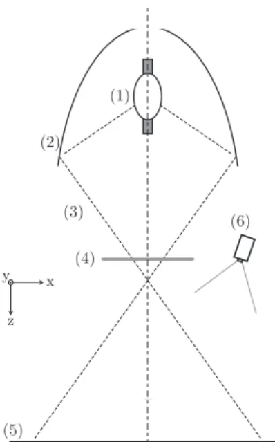
The studied image furnace is mounted with a 4 kW xenon arc lamp (Fig. 1). The lamp is set at the first focus of the elliptical mirror (semi major axis: 430 mm, semi minor axis: 205 mm). The elliptical mirror concentrates radiative power towards its second focus. To map the inci-dent heat flux, a screen is set on the beams’ trajectory to intercept them. As beams energy is absorbed by the screen, its temperature increases. The temperature variations are recorded by a 320 ! 240 IR camera with a working range between 8 and 12lm. Screen exposure is controled by a shutter placed on the light trajectory before the focal spot. The focal spot of this device is known to be 32 cm away from the lamp house casing.
In order to have a flat emissivity of 0.79 in the camera working range, one side of the screen was painted with a black paint. Temperature was monitored on the painted side of the screen. Far from the focal spot, the painted side of the screen was illuminated (Fig. 1). At the focal spot, the bare steel side of the screen was illuminated reducing the absorbed energy by a factor of about 2 (Fig. 2).
Nomenclature
Latin symbols
cp screen specific heat capacity (J/kg/K)
dt time between two frames (s) e screen thickness (m)
h convective heat transfer coefficient (W/m2/K) ~n normal vector ( ) T temperature ("C) t time (s) Greek symbols a absorptivity ( ) dT temperature difference ("C) D Laplacian operator (1/m2) ! emissivity ( )
k screen thermal conductivity (W/m/K) q screen density (kg/m3)
r Stefan Boltzmann constant (W/m2/K4) / incident heat flux (W/m2)
Subscripts
i frame pixel index in x direction j frame pixel index in y direction ols estimated using ordinary least square p paint
s bare steel sur surrounding Superscripts
k frame time index n total number of frame T matrix transposition operator ˆ ordinary least square estimator
2.2. Experimental procedure
The proposed inverse method requires transient screen temperature measurements. Indeed it uses the recording of the screen temperature elevation to yield a map of the incident heat flux. In this work, heat flux is mapped at the focal spot and also at several distances from the focal spot: 50, 75, 100, 125 and 150 cm. In order to assess repeatability, each measurement was repeated twice.
For every run the following experimental procedure was observed:
" the screen and the camera are positioned, " he shutter is closed,
" lamp is turned on,
" 10 min are waited for in order to get the lamp and lamp house thermally stable,
" the camera is started, " the shutter is opened,
" the acquisition is turned off once critical temperatures are reached,
" the shutter is closed.
2.3. Experimental precautions
Because the camera was off the optical axis of the sys-tem, the pictures had to be corrected using a projective transformation before computing the incident heat flux.
In order to later simplify the problem, the screens were chosen to be thin and made out of a conductive material, so that temperature is almost constant in their thicknesses. Here, a 0.8 mm thick stainless steel square plate (304L steel) was used to produce the screens.
In cases where the screen is far from the focal spot
(Fig. 1), its temperature does not increase much and its
physical properties are assumed to remain constant. This assumption implies that the screen temperature does not increase beyond reasonable bounds: 80"C. This tempera-ture was chosen to keep the screen thermal conductivity variation below 10%. In this configuration, under moderate heat flux, the exposed side of the screen is painted black.
At the focal spot (Fig. 2), screen temperature increases sharply up to 300"C within 3 s after which acquisition is stopped. Screen physical property variations was taken into account. Bare steel was exposed to incident heat flux, in order to take advantage of its reduced surface absorptiv-ity and reduce the temperature increase speed so enough frames could be acquired before the screen reached 300"C. Temperature was monitored on the other side that was painted black.
A Gardon radiometer was used to measure incident heat flux on the screen at different positions. These measure-ments allowed validation of the established inverse method results.
In our problem, it is critical to know several key spectral properties: the screen absorptivities with respect to the lamp spectrum and the screen emissivity with respect to
(1) (2) (3) (4) (5) (6) y x z
Fig. 1. Experimental apparatus schematics, defocused configuration. (1) 4 kW xenon arc lamp, (2) elliptical mirror, (3) a ray, (4) shutter, (5) screen, (6) camera, black line paint.
(1) (2) (3) (4) (5) (6)
Fig. 2. Experimental apparatus schematics, focal spot configuration. (1) 4 kW xenon arc lamp, (2) elliptical mirror, (3) a ray, (4) shutter, (5) screen, (6) camera, black line paint.
Table 1
Physical properties of the screen.
Symbol Name Value Dimension
ap Paint absorptivity 0.90
as Steel absorptivity 0.48
!p Paint emissivity 0.79
!s Steel emissivity 0.48
q Steel density 7900 kg/m3
k0 Steel thermal conductivity 15 W/m/K
cp0 Steel heat capacity 500 J/kg/K
the camera range. These properties were measured using a spectrometer and are available inTable 1.
3. Direct model
In order to accurately describe the screen temperature evolution, the direct model has to account for interception of the incident heat flux, conduction inside of the screen, convective and radiative heat loss on the two faces. In this case, the temperature of the screen is governed by a classic 3D transient conduction model:
qcp@T
@t ¼ kDT ð1Þ
The set of boundary conditions are based on the heat flux continuity. On the upper surface of the screen, incident heat flux, convective and radiative heat loss contribute to the heat flux:
&krT '~n ¼ &ap/ þ hðT & TsurÞ þ !prðT4& T4surÞ ð2Þ
With a surrounding temperature Tsurof 20"C.
On the lower surface of the screen, convective and radia-tive heat losses govern the heat flux:
&krT '~n ¼ hðT & TsurÞ þ !srðT4& T4surÞ ð3Þ
On the side of the screen, thermal insulation can be assumed:
&krT '~n ¼ 0 ð4Þ This classical conduction model can be simplified. Indeed, temperature inside the screen might be uniform in its thickness because the screen is very thin and made out of conductive material. Radiative Biot number based on the screen thickness can be calculated (Eq.(5)). Under the most severe circumstances using/max, the Biot number
remains below 0.1. Therefore, the temperature of the screen can be assumed to be homogeneous in its thickness. Biot ¼as/maxe
kdT ¼ 0:090 ð5Þ The direct model can be simplified into a 2D transient model by inserting upper and lower surface boundary con-ditions (Eqs.(2) and (3)) as source terms in Eq.(1): qcp@T @t ¼ kDT þ ap/ e & 2h e ðT & TsurÞ
&ð!pþ !e sÞrðT4& T4surÞ ð6Þ
With the boundary condition on the side of the screen: &krT '~n ¼ 0 ð7Þ
4. Inverse model
The inverse model (Eq.(8)) was built based on the direct model. It enables the calculation of the incident heat flux/ and the convective heat transfer coefficient h for each pixel. Thus it yields a map of the incident heat flux. The idea behind
the inverse model is to calculate the gap (called observable yk
i;j) between the measured increase in temperature and the
contribution of heat diffusion and radiation losses. This gap is directly associated to the contribution of the incident heat flux and the convective loss. Then using ordinary least square method (Orlande et al., 2011), heat flux and convec-tive heat transfer coefficient are computed to minimize this gap. Thus, the best fitting heat flux ^/i;jand convective heat
transfer coefficient ^hi;jare determined for each pixel. In the
present work, for the sake of simplicity, it is assumed that both/ and h are constant in time for a given pixel.
The observable yk
i;jcan be written for each pixel at each
time step as follows: yk
i;j¼ Tkþ1i;j & Tki;j& dt
k qcpDT k i;j & dtð!pqcþ !sÞr pe ððT k i;jþ 273Þ 4 & ðTsurþ 273Þ4Þ ð8Þ
where the Laplacian operator is computed using central finite differences scheme:
DTk
i;j¼ Tkiþ1;jþ Tki&1;j& 4Tki;jþ Tki;jþ1þ Tki;j&1 ð9Þ
For a given pixel, the observable is written as follows:
yi;j¼ y1 i;j .. . yk i;j .. . yn&1 i;j 0 B B B B B B B B B @ 1 C C C C C C C C C A ð10Þ
A sensitivity matrix Xi;j has to be built and inversed for
every pixel. This matrix is the mathematical object which contains the contribution of the incident heat flux and the convective loss.
Xi;j¼ dta qcpe & 2dt qcpeðT 1 i;j& TsurÞ
.. . .. . dta qcpe & 2dt qcpeðT k
i;j& TsurÞ
.. . .. . dta qcpe & 2dt qcpeðT n&1 i;j & TsurÞ
0 B B B B B B B B B @ 1 C C C C C C C C C A ð11Þ
Then, the system can be inverted using simple matrix operations yielding the incident heat flux and the convec-tive coefficient maps:
^ /i;j
^ hi;j
!
¼ ðXTi;jXi;jÞ&1XTi;jyi;j ð12Þ
The inverse method approach has two major advantages that are underlined here. First, on the contrary to CCD cam-era heat flux measurements, it does not require an external scaling factor. This factor being most of the time provided by a radiometer (Guesdon et al., 2006; Sarwar et al., 2014).
Second, distance temperature measurement encounters a reflexion problem. Indeed when the target is exposed to an incident heat flux, a fraction of this heat flux is reflected toward the captor. Thus the measured temperature is the sum of the actual temperature and the reflected heat flux contribution. Precaution has to be taken in order to accu-rately monitor temperature (Hernandez et al., 2004;
Ballestrı´n et al., 2006). In the present work, by building
the observable using temperatures differences, the additive contribution of the reflected heat flux to the monitored tem-perature is nullified.
The thermal properties of the target material were set as follows. As stated before, the screen temperature remains relatively low. It allows to reasonably assume that screen physical properties are constant. Values of the screen ther-mal conductivity and heat capacity can be found in
Table 1. On the contrary, at the focal spot, screen
temper-ature increases sharply up to 300"C. Thus physical proper-ties could not be assumed to be constant and the following correlations (Graves et al., 1991) were used to describe screen thermal conductivity and heat capacity evolution with temperature: kðT ðKÞÞ ¼ 7:9318 þ 0:023051T & 6:4166 ! 10&6T2W=m=K ð13Þ CpðT ðKÞÞ ¼ 426:7 þ 1:700 ! 10&1T þ 5:200 ! 10&5T2J=kg=K ð14Þ 5. Results
It is common in the inverse method field to check the inverse algorithm capabilities with simulated values
(Fan et al., 2009). The direct model was computed with a
prescribed heat flux. Then noise was added to the produced temperature data and finally the inverse algorithm was run. The agreement between actual values and estimated values of the incident heat flux was very good. From there, heat flux distribution were estimated from IR measurements for various distances ranging from z = 0 to z = 150 cm from the focal spot.
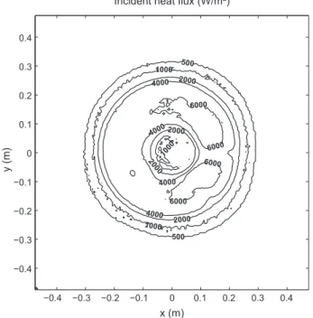
Fig. 3 reports the determined heat flux contour map
100 cm away from the focal spot. One can see that the inci-dent heat flux has a ring shape with a higher heat flux on the right hand side of the map. These discrepancies are attributed to error in the geometrical adjustment of the lamp and the mirror.
A Gardon radiometer was used to measure heat flux along the horizontal and vertical axes as a test to validate the inverse method estimation. Figs. 4 and 5compare the inverse method results with Gradon radiometer measure-ments. Both methods yield very close results. Moreover
x (m)
y (m)
Incident heat flux (W/m²)
500 1000 2000 4000 6000 6000 6000 6000 4000 2000 1000 500 1000 2000 4000 4000 2000 −0.4 −0.3 −0.2 −0.1 0 0.1 0.2 0.3 0.4 −0.4 −0.3 −0.2 −0.1 0 0.1 0.2 0.3 0.4
Fig. 3. Heat flux mapping 1 m away from the focal spot.
−30 −20 −10 0 10 20 30 0 2 4 6 x axis (cm) Incident heat flux (kW/m 2)
Fig. 4. Heat flux 1 m away from the focal spot on the x axis. Continuous line from inverse method, crosses with error bars from Gardon radiometer. −30 −20 −10 0 10 20 30 0 2 4 6 y axis (cm) Incident heat flux (kW/m 2)
Fig. 5. Heat flux 1 m away from the focal spot on the y axis. Continuous line from inverse method, crosses with error bars from Gardon radiometer.
the inverse method provides at a time higher spatial resolu-tion heat flux map than the Gardon radiometer measurements.
Fig. 6 reports the determined heat flux distribution at
the focal spot. The spatial distribution has a maximum of 1335 kW/m2and a diameter of about 3 cm.Fig. 7reports the heat flux distribution along x and y axes. These very similar distributions exhibit a Gaussian shape, which is congruent with literature (Sarwar et al., 2014; Petrasch
et al., 2007; Llorente et al., 2011).
The beam total power is obtained by integrating the heat flux over the screen surface.Fig. 8reports the beam power variation as a function of the distance of the target to the focal spot. The incident power away from the focal spot exhibits small variations of ±5% around an average value
of 966 W. The accuracy of the presented measurements are thought to be very good.
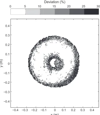
Repeatability was assessed using the two measurements made for each distance. Fig. 9 reports the deviation between two runs: it is lower than 5% in the regions where signal-to-noise ratio is good i.e. area with high incident heat flux. The discrepancy increases in low heat flux areas, which can be explained by the fact that the temperature rise is small in these regions: in this case, the sensibility coeffi-cient associated to convective heat loss tends towards zero (Eq.(15)) which lowers inverse method predictions quality and therefore repeatability.
lim
Tk i;j!Tsur&
2dt qcpðTki;jÞeðT
k
i;j& TsurÞ ¼ 0 ð15Þ
x (m)
y (m)
Incident heat flux (kW/m²)
100 250 500 1250 1000 750 1000 750 500 250 100 005 250 100 500 250 100 −0.02 −0.01 0 0.01 0.02 −0.02 −0.01 0 0.01 0.02
Fig. 6. Heat flux mapping at the focal spot.
−4 −2 0 2 4 0 500 1000 1500 Axis length (cm) Incident heat flux (kW/m 2)
Fig. 7. Heat flux distribution at the focal spot. Continuous line x axis, dashed line y axis.
−25 0 25 50 75 100 125 150 175 800
900 1000 1100
Distance from the focal spot (cm)
Po
w
er
(W)
Fig. 8. Incident power for all runs. Dot individual value, continuous line average value. x (m) y (m) −0.4 −0.3 −0.2 −0.1 0 0.1 0.2 0.3 0.4 −0.4 −0.3 −0.2 −0.1 0 0.1 0.2 0.3 0.4 Deviation (%) 0 5 10 15 20 25 30
6. Conclusion and perspectives
In this paper, inexpensive and easy to handle experi-ments were used to rapidly map the heat flux of a solar con-centrating device. A screen made of a thin widespread painted steel plate was exposed to the incident heat flux. An IR camera was used to record the screen temperature field. IR images sequences were processed using basic inverse method approach and yield incident heat flux distri-bution. As the screen spectral properties were known, no external scaling factor was needed.
Results obtained far from the focal spot were validated by comparison with Gardon radiometer readings: the agreement between the two methods is very good. The computed beam total power has also been shown to be the same for several distances of the screen to the focal spot. Finding that total power is conservative is a token of the good quality of the proposed method.
In this work, the inverse method was used on a basic level. Using more advanced techniques, the incident heat flux can be further characterized. Among the critical possi-ble improvements, time variability of the heat flux is of note. Indeed using more sophisticated approaches
(Mohammadiun et al., 2011; Shi et al., 2013; Park and
Jung, 2001), it would be possible to compute a time
depen-dent incidepen-dent heat flux and convective heat transfer coeffi-cient for every pixel.
Another point is the IR camera resolution. In our case the camera resolution was quite low: 320 ! 240. A greater resolution would lead to a more precise heat flux map and to a better calculation of the Laplacian operator, reducing the impact of noise on the computed heat flux.
Acknowledgements
This work was funded by the French “Investments for the future” program managed by the National Agency for Research under contract ANR-10-LABX-22-01. We would like to thank Olivier Fudym for his help in operating the IR camera and Mickael Ribeiro for his technical support.
References
Authier, O., Ferrer, M., Mauviel, G., Khalfi, A.-E., Lede, J., 2009. Wood fast pyrolysis: comparison of Lagrangian and Eulerian modeling approaches with experimental measurements. Ind. Eng. Chem. Res. 48 (10), 4796 4809.http://dx.doi.org/10.1021/ie801854c, wOS:000266081 300016.
Ballestrı´n, J., Rodrı´guez-Alonso, M., Rodrı´guez, J., Can˜adas, I., Barbero, F.J., Langley, L.W., Barnes, A., 2006. Calibration of high-heat-flux sensors in a solar furnace. Metrologia 43 (6), 495.http://dx.doi.org/ 10.1088/0026-1394/43/6/003, <http://iopscience.iop.org/0026-1394/ 43/6/003>.
Codd, D.S., Carlson, A., Rees, J., Slocum, A.H., 2010. A low cost high flux solar simulator. Sol. Energy 84 (12), 2202 2212.http://dx.doi.org/ 10.1016/j.solener.2010.08.007, <http://www.sciencedirect.com/science/ article/pii/S0038092X10002665>.
Fan, C., Sun, F., Yang, L., 2009. Simple numerical method for multidimensional inverse identification of heat flux distribution. J. Thermophys. Heat Transfer 23 (3), 622 629. http://dx.doi.org/ 10.2514/1.38446, wOS:000268300300023.
Fang, Z., Xie, D., Diao, N., Grace, J.R., Jim Lim, C., 1997. A new method for solving the inverse conduction problem in steady heat flux measurement. Int. J. Heat Mass Transfer 40 (16), 3947 3953.http:// dx.doi.org/10.1016/S0017-9310(97)00046-X, <http://www.sciencedirect. com/science/article/pii/S001793109700046X>.
Graves, R.S., Kollie, T.G., McElroy, D.L., Gilchrist, K.E., 1991. The thermal conductivity of AISI 304l stainless steel. Int. J. Thermophys. 12 (2), 409 415.http://dx.doi.org/10.1007/BF00500761, <http://link. springer.com/article/10.1007/BF00500761>.
Guesdon, C., Alxneit, I., Tschudi, H.R., Wuillemin, D., Sturzenegger, M., 2006. 1 kW imaging furnace with in situ measurement of surface temperature. Rev. Sci. Instrum. 77 (3), 035102. http://dx.doi.org/ 10.1063/1.2173844, wOS:000236739100040.
Hernandez, D., Olalde, G., Gineste, J.M., Gueymard, C., 2004. Analysis and experimental results of solar-blind temperature measurements in solar furnaces. J. Sol. Energy Eng.-Trans. ASME 126 (1), 645 653.
http://dx.doi.org/10.1115/1.1636191, wOS:000189287100013. Imhof, A., 1997. Decomposition of limestone in a solar reactor. Renew.
Energy 10 (2 3), 239 246. http://dx.doi.org/10.1016/0960-1481(96) 00072-9, <http://www.sciencedirect.com/science/article/pii/096014819 6000729>.
Kaushika, N., Kaneff, S., 1987. Flux distribution and intercept factors in the focal region of paraboloidal dish concentrators. In: Proc. ISES Solar World Congress, vol. 2, Hamburg, pp. 1607 1611.
Llorente, J., Ballestrin, J., Vazquez, A.J., 2011. A new solar concentrating system: description, characterization and applications. Sol. Energy 85 (5), 1000 1006. http://dx.doi.org/10.1016/j.solener.2011.02.018, wOS:000290644000029.
Mohammadiun, M., Rahimi, A.B., Khazaee, I., 2011. Estimation of the time-dependent heat flux using the temperature distribution at a point by conjugate gradient method. Int. J. Therm. Sci. 50 (12), 2443 2450.
http://dx.doi.org/10.1016/j.ijthermalsci.2011.07.003, < http://www.sci-encedirect.com/science/article/pii/S1290072911002134>.
Orlande, H.R.B., Fudym, O., Maillet, D., Cotta, R.M. (Eds.), 2011. Thermal Measurements and Inverse Techniques. CRC Press, Boca Raton, FL.
Park, H.M., Jung, W.S., 2001. On the solution of multidimensional inverse heat conduction problems using an efficient sequential method. J. Heat Transfer-Trans. ASME 123 (6), 1021 1029.http://dx.doi.org/ 10.1115/1.1409260, wOS:000172645400001.
Petrasch, J., Coray, P., Meier, A., Brack, M., Haeberling, P., Wuillemin, D., Steinfeld, A., 2007. A novel 50 kW 11,000 suns high-flux solar simulator based on an array of xenon arc lamps. J. Sol. Energy Eng.-Trans. ASME 129 (4), 405 411.http://dx.doi.org/10.1115/1.2769701, wOS:000250637900008.
Sarwar, J., Georgakis, G., LaChance, R., Ozalp, N., 2014. Description and characterization of an adjustable flux solar simulator for solar thermal, thermochemical and photovoltaic applications. Sol. Energy 100, 179 194.http://dx.doi.org/10.1016/j.solener.2013.12.008, wOS:00 0331007700018.
Shi, Y.-A., Zeng, L., Qian, W.-Q., Gui, Y.-W., 2013. A data processing method in the experiment of heat flux testing using inverse methods. Aerospace Sci. Technol. 29 (1), 74 80. http://dx.doi.org/10.1016/ j.ast.2013.01.009, <http://www.sciencedirect.com/science/article/pii/ S1270963813000126>.