Hydrate Mitigation in Sour and Acid Gases

(1)

HAL Id: tel-01139496

https://pastel.archives-ouvertes.fr/tel-01139496

Submitted on 5 Apr 2015

HAL is a multi-disciplinary open access archive for the deposit and dissemination of sci-entific research documents, whether they are pub-lished or not. The documents may come from teaching and research institutions in France or

L’archive ouverte pluridisciplinaire HAL, est destinée au dépôt et à la diffusion de documents scientifiques de niveau recherche, publiés ou non, émanant des établissements d’enseignement et de recherche français ou étrangers, des laboratoires

Martha Hajiw

To cite this version:

Martha Hajiw. Hydrate Mitigation in Sour and Acid Gases. Chemical and Process Engineering. Ecole Nationale Supérieure des Mines de Paris, 2014. English. �NNT : 2014ENMP0042�. �tel-01139496�

(2)

T

H

E

S

École doctorale n° 432 : Sciences des Métiers de l’Ingénieur

présentée et soutenue publiquement par

Martha HAJIW

le 24 novembre 2014

Etude des Conditions de Dissociation des Hydrates de Gaz en Présence de

Gaz Acides

Hydrate Mitigation in Sour and Acid Gases

Doctorat ParisTech

T H È S E

pour obtenir le grade de docteur préparée dans le cadre d’une cotutelle entre

l’École nationale supérieure des mines de Paris

et l’université Heriot Watt

Spécialité “ Energétique et Procédés ”

Directeur de thèse : Christophe COQUELET Co-directeur de la thèse : Antonin CHAPOY

T

H

È

S

E

Jury

M. Jean-Michel HERRI Président

M. Jean-Noel JAUBERT Rapporteur

M. Georgios KONTOGEORGIS Rapporteur

M. Florian DOSTER Examinateur

M. Pierre DUCHET-SUCHAUX Examinateur

M. Gerhard LAUERMANN Examinateur

M. Antonin CHAPOY Directeur de thèse

(3)

(4)

ABSTRACT

While global demand for energy is increasing, it is mostly covered by fossil energies, like oil and natural gas. Principally composed of hydrocarbons (methane, ethane, propane...), reservoir fluids contain also impurities such as carbon dioxide, hydrogen sulphide and nitrogen. To meet the request of energy demand, oil and gas companies are interested in new gas fields, like reservoirs containing high concentrations of acid gases.

Natural gas transport is done under high pressure and these fluids are also saturated with water. These conditions are favourable to hydrates formation, leading to pipelines blockage. To avoid these operational problems, thermodynamic inhibitors, like methanol or ethanol, are injected in lines.

It is necessary to predict with more accuracy hydrates boundaries in different systems to avoid their formation in pipelines for example, as well as vapour liquid equilibria (VLE) in both sub-critical regions. Phase equilibria predictions are usually based on cubic equations of state and applied to mixtures, mixing rules involving the binary interaction parameter are required. A predictive model based on the group contribution method, called PPR78, combined with the Cubic – Plus – Association (CPA) equation of state has been developed in order to predict phase equilibria of mixtures containing associating compounds, such as water and alcohols.

To complete database for multicomponent systems with acid gases, VLE and hydrate dissociation point measurements have been conducted.

The developed model, called GC-PR-CPA, has been validated for binary systems and applied for different multicomponent mixtures. Its ability to predict hydrate stability zone and mixing enthalpies has also been tested. It has been found that the model is generally in good agreement with experimental data.

(5)

(6)

A mes parents

A ma sœur Stéphanie et mon frère Lucas

A Jean

(7)

(8)

ACKNOWLEDGMENTS

This work is the result of a joint PhD between the Centre of Gas Hydrates in Heriot Watt University and the Centre Thermodynamic of Processes in Mines ParisTech.

Je souhaiterais dans un premier temps remercier mes deux directeurs de these, Antonin Chapoy et Christophe Coquelet pour leur accueil au sein de leur laboratoire respectif, pour nos nombreux échanges et pour leur soutien durant ces trois années de thèse.

I would like to thank Pr. Georgios Kontogeorgis, Pr. Jean-Noel Jaubert and Dr. Florian Doster for accepting to review my thesis and for their advices.

I would also like to thank Pr. Jean-Michel Herri for accepting to be the chairman of the thesis committee and M. Pierre Duchet-Suchaux and M. Gerhard Lauermann for taking part to the jury but also for our discussions during the meetings we had.

I spent unforgatable eighteen months in Scotland thanks to a great team in IPE. I am particularly thankful to Pr. Bahman Tohidi for welcoming me in the Centre of Gas Hydrates, to Rod Burgass and Jebraeel Gholinezhad who helped me a lot in the lab. Thanks to my colleagues and friends, I enjoyed my stay in Edinburgh. It would not have been the same without you, my “sister” Diana, Ramin, Chuks, Foroogh, Luis, Mohamed, Mahdi, Morteza, Babak, Mojtaba and Reza. I was also lucky to find a second family in the Ukrainian club: thank to the AUGB and the Ukrainian church for welcoming me so warmly.

Bien que moins dépaysant, mon séjour à Fontainebleau n’en a pas été moins agréable et ce grâce au formidable accueil qui m’a été reservée (toute ironie mise à part). J’exprime par ces quelques lignes toute ma sympathie pour les membres du CTP: Jocelyne et Marie-Claude pour m’avoir aidée à me dépêtrer des tracas administratifs, Alain, Pascal, Snaide, Elodie, Eric, David et Hervé pour avoir tour à tour ou ensemble persevéré à faire tourner des manips qui fuient, mes collègues thésards ou anciens thésards, Marco, Fan et Jamal, pour leur soutien (oui « la thèse nuit gravement à la santé » mais « on bosse dur »), Céline, Paolo, Eric et Mauro pour nos discussions pas

(9)

toujours scientifiques et enfin, mais pas des moindres, Elise pour son aide, ses conseils et pour nos virées shopping.

Je remercie très chaleureusement mes parents qui m’ont toujours soutenue et encouragée dans les études, ma sœur Stéphanie et mon frère Lucas mais aussi toute la famille Hajiw, Krupiak et Zubko.

Je remercie tous mes amis et plus particulièrement Emmanuelle ainsi que la communauté ukrainienne d’Algrange qui m’a vue grandir et qui suit mon parcours depuis tant d’années.

Enfin j’adresse mes plus vifs remerciements à Jean pour son indéfectible soutien durant ma thèse et surtout lors de la rédaction de ce manuscrit. Merci aussi à sa famille.

(10)

(11)

(12)

LIST OF TABLES

Table 1.1: Example of natural gas composition ... 10

Table 1.2: Example of properties of flue gases from thermal power plants ... 19

Table 1.3: Composition of the mild carbon steel X65... 25

Table 1.4: Geometry of cages in the three hydrates structures ... 28

Table 2.1: VLE status of the bibliographic study ... 37

Table 2.2: Composition of each component (mole %) of mixture MIX 1 ... 41

Table 2.3: Materials used for VLE measurements ... 42

Table 2.10: Pressure transducers calibration ... 48

Table 2.11: Temperature probes calibration ... 49

Table 2.12: Experimental bubble points of the 95% CO2 + 5% Ar binary system ... 52

Table 2.13: Experimental bubble points of MIX 1... 53

Table 2.14: Experimental hydrate dissociation conditions in the presence of distilled water of the system 95% CO2 + 5% Ar ... 54

Table 2.15: Experimental hydrate dissociation conditions in the presence of distilled water of MIX 1 ... 54

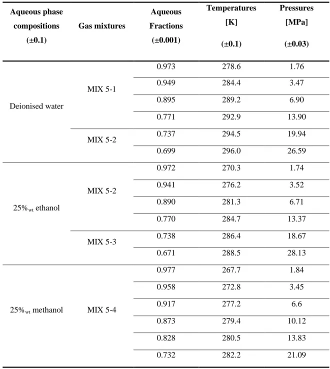
Table 2.16: Experimental hydrate dissociation conditions with gas mixtures MIX 5 in the presence of distilled water and different aqueous solutions ... 55

Table 2.17: Experimental hydrate dissociation conditions with gas mixtures MIX 6 in the presence of different aqueous solutions ... 57

Table 2.18: Experimental hydrate dissociation conditions with gas mixtures MIX 7 in the presence of different aqueous solutions ... 59

Table 2.19: Experimental hydrate dissociation conditions in the presence of distilled water of 80%mol CH4 +20%mol H2S system ... 61

Table 3.1: Classical cubic equations of state ... 68

Table 3.2: Parameters used in the cubic equations of state. ... 69

Table 3.3: Parameters of the attractive parameter ... 70

Table 3.4: Parameters of the co-volume ... 71

Table 3.5: Reference properties for structures I and II hydrates ... 76

Table 3.6: Parameters used in the PR-CPA EoS. ... 77

Table 3.7: Association schemes for associating components ... 80

Table 3.8: Groups defined in the PPR78 EoS. ... 83

Table 3.9: Group parameters in the PPR78 EoS. Green: parameters available. Red: no parameters ... 85

Table 4.1: PR-CPA parameters for water and alcohol ... 93

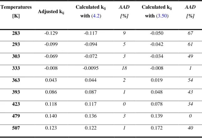
Table 4.2: Comparison between adjusted kij temperature by temperature, calculated kij with PPR78 and calculated kij with the GC-PR-CPA EoS for the binary system methane-water. ... 97

Table 4.3: Comparison between adjusted kij temperature by temperature, calculated kij with PPR78 and calculated kij with the GC-PR-CPA EoS for the binary system benzene-water. ... 98

Table 4.4: Group interaction parameters with water ... 99

(17)

Table 4.7: Group interaction parameters for alcohols ... 103 Table 5.1: Deviations between the GC-PR-CPA model and experimental data for normal alkanes – water binary systems ... 108 Table 5.2: n-Pentane and n-hexane solubility in water ... 110 Table 5.3: Deviations between the GC-PR-CPA model and experimental data for branched alkanes – water binary systems ... 112 Table 5.4: Deviations between the GC-PR-CPA model and experimental data for alkenes – water binary systems ... 113 Table 5.5: Deviations between the GC-PR-CPA model and experimental data for naphthenic hydrocarbons – water binary systems ... 115 Table 5.6: Cyclohexane and methylcyclohexane solubility in water ... 116 Table 5.7: Deviations between the GC-PR-CPA model and experimental data for aromatic hydrocarbons – water binary systems ... 116 Table 5.8: Benzene, toluene and ethylbenzene solubility in water ... 117 Table 5.9: Deviations between the GC-PR-CPA model and experimental data for acid gases – water and inert gases – water binary systems ... 120 Table 5.10: Deviations between the GC-PR-CPA model and experimental data for alcohol – water binary systems ... 123 Table 5.11: Deviations between the GC-PR-CPA model and experimental data for methane – methanol binary system ... 125 Table 5.12: Deviations between the GC-PR-CPA model and experimental data for normal alkanes – methanol binary system ... 125 Table 5.13: Deviations between the GC-PR-CPA model and experimental data for branched alkanes – methanol binary systems ... 126 Table 5.14: Deviations between the GC-PR-CPA model and experimental data for naphthenic hydrocarbons – methanol binary systems ... 128 Table 5.15: Deviations between the GC-PR-CPA model and experimental data for aromatic hydrocarbons – methanol binary systems ... 129 Table 5.16: Deviations between the GC-PR-CPA model and experimental data for acid gases – methanol and inert gases – methanol binary systems ... 130 Table 5.17: Deviations between the GC-PR-CPA model and experimental data for alcohols – methanol binary systems ... 131 Table 5.18: Deviations between the GC-PR-CPA model and experimental data for methane – ethanol and ethane – ethanol binary systems ... 132 Table 5.19: Deviations between the GC-PR-CPA model and experimental data for normal alkanes – ethanol binary systems ... 132 Table 5.20: Deviations between the GC-PR-CPA model and experimental data for branched alkanes – ethanol binary systems ... 133 Table 5.21: Deviations between the GC-PR-CPA model and experimental data for naphthenic hydrocarbons – ethanol binary systems ... 134 Table 5.22: Deviations between the GC-PR-CPA model and experimental data for aromatic hydrocarbons – ethanol binary systems ... 135 Table 5.23: Deviations between the GC-PR-CPA model and experimental data for carbon dioxide – ethanol and inert gases – ethanol binary systems ... 136 Table 5.24: Deviations between the GC-PR-CPA model and experimental data for alkanes – alcohols binary systems ... 137 Table 5.25: Deviations between the GC-PR-CPA model and experimental data for alcohol –

(18)

Table 5.27: Deviations between the GC-PR-CPA model and experimental data for MIX 8 ... 138 Table 5.28: Deviations between the GC-PR-CPA model and experimental data for MIX 9 ... 139 Table 5.29: Composition of each component (mole %) of mixture MIX 10 ... 140 Table 5.30: Deviations between the GC-PR-CPA model and experimental data for MIX 10 . 140

(19)

(20)

LIST OF FIGURES

Figure 1.1: World oil production and consumption between1987 and 2012 ... 6

Figure 1.2: World Natural Gas production and consumption between1987 and 2012 ... 6

Figure 1.3: World energy consumption by fuel type between 1990 and 2010 and projections for the next 30 years ... 7

Figure 1.4: World Natural Gas reserves at the end of 2011 ... 8

Figure 1.5: World sour and acid gas reserves ... 8

Figure 1.6: Global CO2 emissions from fossil energies from 1960 to 2012 ... 9

Figure 1.7: Example of natural gas phase diagram ... 13

Figure 1.8: Natural gas pipeline network ... 14

Figure 1.9: Natural gas phase envelope and compression conditions ... 16

Figure 1.10: Transport chain ... 16

Figure 1.11: Global carbon dioxide emissions by sector between 1990 and 2010 ... 17

Figure 1.12: Schematic of processes for carbon dioxide capture. ... 18

Figure 1.13: Temperature and pressure conditions of the CCS systems ... 22

Figure 1.14: Phase diagram for different CO2 – N2 mixtures ... 22

Figure 1.15: Hydrogen bonding between five molecules of water. ... 26

Figure 1.16: Hydrates structures ... 27

Figure 1.17: Gas hydrates removed from a pipeline ... 29

Figure 1.18: Known and expected methane hydrates locations in the World ... 30

Figure 2.1: n-Pentane solubility in water at atmospheric pressure ... 38

Figure 2.2: Schematic of apparatus used for bubble point measurements. ... 40

Figure 2.3: Flow diagram of the equipment used for VLE measurements ... 42

Figure 2.4: Schematic of apparatus used for hydrate dissociation point measurements. ... 44

Figure 2.5: Schematic flow diagram of the apparatus ... 45

Figure 2.6: Pressure – mass diagram to determine the bubble point at constant temperature ... 50

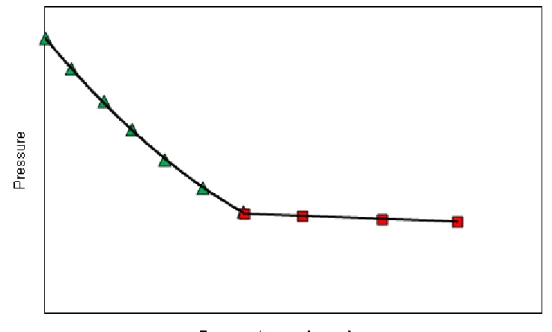
Figure 2.7: Pressure – temperature diagram for estimating hydrate dissociation point ... 51

Figure 3.1: Variation of the alpha function ... 70

Figure 3.2: Boltzmann probability factor versus r ... 74

Figure 3.3: Shape of Lennard-Jones potential ... 74

Figure 3.4: Schematic of the notation used in Kihara potential. ... 75

Figure 3.5: Illustration of site-to-site distance and orientation and square-well potential ... 78

Figure 3.6: Water solvation of carbon dioxide ... 81

Figure 3.7: Temperature dependence of the kij parameter ... 82

Figure 4.1: CH4 solubility in water at 310.93 K, 423.15 K and 473.15 K ... 95

Figure 4.2: Water content in the vapour phase of the methane and water binary system at 423.15K ... 95

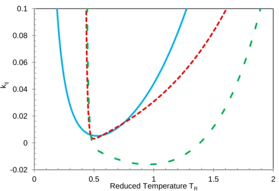
Figure 4.3: Shape of the methane – water kij versus methane reduced temperature ... 96

Figure 4.4: Shape of the benzene – water kij versus benzene reduced temperature ... 96

Figure 5.1: Ethane solubility in water at 313.15 K, 373.15 K and 393.15 K ... 109

Figure 5.2: n-pentane and n-hexane solubilities in water at atmospheric pressure ... 110

Figure 5.3: Water content in ethane at 283.11 K, 293.11 K and 303.15 K ... 111

Figure 5.4: Water solubility in n-hexane at atmospheric pressure ... 112

Figure 5.5: Ethylene solubility in water at 310.93 K, 327.59 K and 344.26 K ... 114

Figure 5.6: Cyclohexane and Methylcyclohexane solubilities in water at atmospheric pressure ... 115

(21)

Figure 5.8: Toluene and Ethylbenzene solubilities in water at 0.5 MPa ... 119

Figure 5.9: Carbon dioxide solubility in water at 288.26 K, 298.28 K, 308.2 K and 318.23 K121 Figure 5.10: Hydrogen sulphide solubility in water at 393.15 K, 423.15 K and 453.15 K ... 121

Figure 5.11: Water content in carbon dioxide at 373.15 K, 393.15 K, 413.15 K and 433.15 K ... 122

Figure 5.12: Water content in carbon dioxide at 366.48 K,394.26 K and 422.04 K ... 122

Figure 5.13: Phase equilibria of the binary system water – ethanol at 313.15 K and 323.15 K ... 124

Figure 5.14: Freezing points of the binary system water – methanol at 313.15 K ... 124

Figure 5.15: Phase equilibria of the binary system i-butane – methanol at 313.06 K and 323.15 K ... 127

Figure 5.16: Phase equilibria of the binary system cyclohexane – methanol at 293.15 K, 303.15 K and 313.15 K ... 128

Figure 5.17: Phase equilibria of the binary systems toluene – methanol and p-xylene – methanol at 313.15 K ... 129

Figure 5.18: Phase equilibria of the binary systems n-butanol – methanol at 298.15 K ... 131

Figure 5.19: Phase equilibria of the binary systems cyclohexane – ethanol at 298.15 K ... 134

Figure 5.20: Phase equilibria of the binary systems o-xylene – ethanol at 308.15 K ... 135

Figure 5.21: Compositions of methane and ethane in organic phase of MIX 10 at 298.1 K ... 141

Figure 5.22: Compositions of n-heptane, n-decane and toluene in organic phase of MIX 10 at 298.1 K ... 142

Figure 5.23: Compositions of methane in vapour phase of MIX 10 at 298.1 K ... 142

Figure 5.24: Compositions of n-heptane, toluene and water in vapour phase of MIX 10 at 298.1 K ... 143

Figure 5.25: Hydrate dissociation points of 80% methane + 20% hydrogen sulphide system 144 Figure 5.26: Hydrate dissociation points of MIX 5 with deionised water ... 144

Figure 5.27: Hydrate dissociation points of MIX 5 with deionised water, 25%wt ethanol and 25%wt methanol ... 145

Figure 5.28: Hydrate dissociation points of MIX 5 with deionised water, 25%wt methanol and 50%wt methanol ... 145

Figure 5.29: Enthalpies of mixing at atmospheric pressure of the binary system water –propane at 383.2 K and 393.2 K ... 147

Figure 5.30: Enthalpies of mixing at 16.4 MPa of the binary system water – benzene at 581 K and 592 K ... 148

Figure 5.31: Enthalpies of mixing at atmospheric pressure of the binary system water –nitrogen at 373.15 K and 423.15 K ... 149

Figure 5.32: Excess enthalpies at atmospheric pressure of the water – ethanol binary system at 323.15 K. ... 150

Figure 5.33: Total apparent molar thermodynamic quantity of the water – ethanol binary system at 323.15 K ... 150

(22)

(23)

(24)

INTRODUCTION

La demande en énergies fossiles ne cesse de s’accroitre avec l’augmentation de la population mondiale et l’émergence économique de nouveaux pays. Les industries pétrolières et gazières sont confrontées à de nouveaux défis : forage en mer profonde, sources non-conventionnelles et gaz acides (dioxyde de carbone et le sulfure d’hydrogène présents en quantités variables dans le gaz naturel). En plus de ces défis technologiques, les énergies fossiles sont aussi émettrices de dioxyde de carbone, gaz à effet de serre qui a un impact non négligeable sur le climat. Une des solutions serait de le capturer et le transporter vers des zones de stockage. Qu’il s’agisse du transport du gaz naturel ou du dioxyde de carbone, de l’eau peut être présente introduisant un risque supplémentaire : la formation d’hydrates de gaz. C’est sur cette problématique que s’appuie cette thèse. Un travail de modélisation a été effectué pour prédire les diagrammes de phases des hydrocarbures, des gaz acides (CO2, H2S) et inertes (N2, H2)

en présence d’eau et d’alcools. Des études expérimentales ont été menées sur des systèmes multi-constituants pour évaluer la capacité du modèle à prédire les équilibres entre phases pour des mélanges complexes et le valider.

(25)

With the growing population and the economic emergence of new countries, the demand in fossil energies is continuously increasing. To meet the demand, oil and gas industries are looking to new types of reservoirs, and therefore face new challenges: deepwater drilling, unconventional oil and gases, acid gases (gases with an important concentration of carbon dioxide and hydrogen sulphide). In addition to these challenges, combustion of fossil fuels is the principal anthropological source of carbon dioxide emissions to the atmosphere. It is considered as the major cause of global warming. A solution proposed is to capture, transport and store carbon dioxide produced in suitable geological reservoirs.

Whether natural gas or carbon dioxide, they are transported with impurities. One of them is water, which may lead to hydrate formation in pipelines. This introduces a serious flow assurance issue, since hydrates may block pipelines.

Chapter 1 presents natural gas and carbon dioxide transportation. The thesis is principally focused on hydrate formation during transportation. Since the systems of interest contain acid gases, it leads to different problems, which may be encountered during transportation. In the presence of water, they intensify the risk of pipeline corrosion and blockage (hydrates formation). To avoid hydrates formation, inhibitors such as methanol, ethanol or glycols are used. Therefore accurate knowledge of mixtures phase equilibria are important for safe operation of pipelines and production/processing/separation facilities.

As part of three industrial projects experimental measurements have been conducted and presented in Chapter 2:

 Hydrate dissociation points and vapour-liquid equilibrium points have been measured for different mixtures to determine the impact of aromatic impurities on acid gas systems, in the case of acid gas injection.

 Hydrate dissociation points of rich CO2 systems have been also measured in the context of carbon dioxide transport in Carbon Capture and Storage (CCS)

 Hydrate dissociation points of different hydrocarbon mixtures in the presence of hydrate inhibitors have been determined in the context of flow assurance

Data generated are used to evaluate and validate the capability of the model to predict phase equilibria of complex systems.

Phase equilibria are predicted with thermodynamic models. Cubic equations of state (EoS), such as the Soave-Redlich-Kwong (SRK EoS) [1] and the Peng-Robinson

(26)

water or alcohols, because they have been developed mainly for hydrocarbons. To improve their ability to predict phase behaviour, none zero binary interaction parameters are introduced. They are adjusted on experimental data for each binary system of interest. In the case of no data are available, there are two solutions: or experimental data are conducted to complete database, or predictive models are used. One of the predictive model available in the literature, the PPR78 model [3], is presented in

Chapter 3, as well as the Cubic-Plus Associtaion EoS [4], suitable for systems containing associating compounds.

In this thesis, a predictive model (called GC-CPA-PR, for Group Contribution – CPA – PR), combining the CPA EoS and the PPR78 model, has been developed and is explained in Chapter 4. The aim is to take into account the hydrogen bonding with the CPA EoS and to have a robust model to predict phase equilibria (VLE, LLE and hydrate stability zone) of different mixtures. Parameters have been adjusted for binary systems with associating compounds (water and alcohols) on experimental data taken from the literature.

Chapter 5 presents the validation of the model. First, predictions are compared to experimental data (VLE and LLE) taken from the literature for binary systems of water and alcohols. Then, the ability of the model to predict phase equilibria of more complex systems is assessed. Finally, the model is tested on hydrate stability zone and enthalpy of mixing predictions. The mixtures are either from the literature or those generated in laboratory and presented in Chapter 2.

(27)

REFERENCES

[1] Soave, G., Equilibrium Constants from a Modified Redlich-Kwong Equation of State. Chemical Engineering Science, 1972. 27(6): p. 1197-&.

[2] Peng, D. and D.B. Robinson, New 2-Constant Equation of State. Industrial & Engineering Chemistry Fundamentals, 1976. 15(1): p. 59-64.

[3] Jaubert, J.N. and F. Mutelet, VLE Predictions with the Peng-Robinson Equation of State and

Temperature Dependent k(ij) Calculated through a Group Contribution Method. Fluid Phase Equilibria,

2004. 224(2): p. 285-304.

[4] Kontogeorgis, G.M., et al., An Equation of State for Associating Fluids. Industrial & Engineering Chemistry Research, 1996. 35(11): p. 4310-4318.

(28)

CHAPTER 1 – NATURAL GAS AND CARBON DIOXIDE

TRANSPORT: PROPERTIES, FEATURES AND PROBLEMS

La consommation en énergies fossiles représente 80% [1.1] de la consommation mondiale en énergies, avec une augmentation de la demande en gaz naturel. Pour répondre à cette demande, les industries s’orientent vers de nouvelles ressources, comme les gaz de schistes ou les gaz naturels à forte teneur en gaz acides. Ces derniers représentent 40% des ressources connues actuellement. Ils contiennent en proportions variables mais conséquentes du dioxyde de carbone et du sulfure d’hydrogène. Or ces composés sont des impuretés qu’il faut séparer des hydrocarbures pour répondre aux exigences techniques nécessaires avant toute commercialisation et utilisation. Il faut donc connaitre les différentes propriétés du gaz naturel pour adapter les conditions de transport.

L’émission de gaz à effet de serre est à l’origine du réchauffement climatique. Les sources anthropiques en sont la principale cause, avec une part importante due à la combustion des énergies fossiles. Les émissions en dioxyde de carbone issues de l’industrie en sont une part non négligeable. Une des solutions étudiées est la capture du dioxyde de carbone et son stockage dans des sites géologiques. Quelque soit la technique de capture, le dioxyde de carbone est récupéré avec des impuretés, qui ont une influence non négligeable sur les propriétés du mélange.

Dans le cas de l’industrie gazière, l’eau est une des plus importantes impuretés à traiter. Elle est aussi présente en quantités variables avec le gaz naturel ou le dioxyde de carbone. En présence de gaz acides et d’un milieu aqueux, les pipelines peuvent se corroder. Le matériau étant détérioré, cela peut être une cause de fuite. La présence d’eau et de petites molécules (méthane, dioxyde de carbone, sulfure d’hydrogène…), dans certaines conditions de pression et de température, est une situation favorable à la formation d’hydrates. Ces structures cristallines peuvent bloquer les pipelines. Le sujet de cette thèse étant centré sur les hydrates de gaz, un rapide descriptif de la corrosion est donné dans la dernière partie avant de décrire plus en détails les caractéristiques des hydrates.

(29)

1.1. INTRODUCTION

The twentieth century has seen an important increase of the fossil energy demand with an annual growth rate for the natural gas of 3% for 30 years [1.2]. They represent today 80% of world energy consumption [1.1]. Figure 1.1 and Figure 1.2 show the world oil

and gas production and consumption between 1987 and 2012. According to the US Energy Information Administration (EIA) the total world energy use is supposed to rise from 524 quadrillion British thermal units (Btu) in 2010 to 820 quadrillion Btu in 2040 [1.3].

Figure 1.1: World oil production (left) and consumption (right) between1987 and 2012

[1.4].

(30)

With the growing population, the demand is still increasing: the EIA foresees a 56% raise in the world energy consumption between 2010 and 2040 (Figure 1.3). This trend is strongest in countries outside the Organization for Economic Cooperation and Development (OECD) with a rise of 90%, while it is just 17% in OECD countries. Moreover, world industrial sector and transport consume half of the energies produced. Despite a decrease of liquid fuels use and an increase of renewable energies and nuclear plant use (plus 2.5 % per year), fossil fuels continue to supply the majority of the world energy demand. Indeed, liquid fuels are the most used in the transport sector and despite of the increasing prices, their used is supposed to rise by 38% from 2010 to 2040.

Figure 1.3: World energy consumption by fuel type between 1990 and 2010 and projections for the next 30 years [1.3].

According to the EIA, natural gas use increases by 1.7% per year. With 116 quadrillion Btu consumed in 2010, the increase is estimated at 64 % with a consumption of 190 quadrillion Btu in 2040. Among all fossil energies, natural gas presents a lot of benefits: low risk since it is not toxic, lower carbon dioxide emissions relative to other fossil fuels and quicker reaction to demand peaks. With the consumption pace, the actual proven reserves (Figure 1.4) are supposed to be enough for 60 years. Oil and gas companies are interested in new gas fields, like shale, coal bed, tight and sour gas.

(31)

Figure 1.4: World Natural Gas reserves at the end of 2011 [1.5]. ■ +10%, ■ from 2 to 5%, ■ from 1 to 1.9%, ■ from 0.1 to 0.9%

40% of these reserves [1.6] are acid and sour gases (Figure 1.5), i.e. the percentage of carbon dioxide and hydrogen sulphide is significant. Middle Eastern and central Asian countries have the most important fields. Their production and transport can be a challenge, due to their corrosiveness in the presence of water, leading to pipelines damages and H2S toxicity. Oil and gas companies are in search of environmentally friendly and gainful methods for dealing with acid and sour gases, as well as low energy consumption.

(32)

Some fields are even ultra-sour, with over 20% of CO2 or H2S. In all cases, these compounds are considered as impurities as well as water usually present in the reservoirs and other elements (e.g. nitrogen, helium...). They are removed by chemical absorption in separation units. Acid gases are commonly removed with different types of amines. For example, the maximum concentration of hydrogen sulphide allowed in treated gas is about 4 ppm [1.8]. They are then compressed and injected into suitable underground formations.

As a result of world’s dependence on fossil energies, the release of carbon into atmosphere is increasing and leads to climate changes. The combustion of fossil fuels generates about 30 gigatons of CO2 per year, or 43% of total CO2 emissions [1.9]. In 2012, Coal represents 43% of total fuel-based CO2 emissions, oil 33% and natural gas 18% [1.10] (see Figure 1.6).

Figure 1.6: Global CO2 emissions from fossil energies from 1960 to 2012 [1.10].

Estimations predict an increase of temperature between 1.0 to 2.1°C per 3600 gigatons of CO2 emitted [1.11]. Even if a solution is found now to stop carbon dioxide emissions, the climate changes are irreversible and last up to 1000 years [1.12]. Fossil energies-based CO2 emissions come from both stationary (e.g. power plant, refinery) and non-stationary systems (e.g. urban transport) [1.9]. Different ways to reduce CO2 emissions in the atmosphere have been proposed. One of the most promising is the Carbon Capture and Storage (CCS). Amines are currently used as chemical solvent in fuel process plants to remove carbon dioxide. But all carbon dioxide capture technologies, existing or future, depend on different factors:

(33)

 CO2 concentration in the gas mixture

 Presence of impurities (water, SOx, NOx...)?

 Temperature and pressure conditions

Then carbon dioxide is transported through pipelines for Enhanced Oil Recovery (EOR), which looks to be the main target for many operators, or to storage sites. The ones actually considered are geologic formations (deep saline aquifers, depleted oil and gas fields...) [1.9].

Whether in natural gas production, carbon dioxide capture or acid gas injection, water may be present. During the different steps in production, transportation and processing, changes in temperature and pressure can lead to water condensation, ice and/or gas hydrates formation.

General information of both natural gas and carbon dioxide, as well as their transportation conditions are presented below. Origins of water, corrosion problem and hydrate formation in pipelines are also explained.

1.2. NATURAL GAS TRANSPORT

1.2.1. What is Natural Gas?

If a natural substance is in gaseous state at IUPAC standard conditions1, it is a

permanent gas. In subsurface rock reservoirs it is hydrocarbons from methane to

butane, carbon dioxide, nitrogen, hydrogen sulphide, hydrogen, helium and argon [1.8]. But the natural gas recovered, contains permanent gases but also heavier hydrocarbons. Compositions depend on reservoir source, history and present conditions. An example of typical composition is given in Table 1.1.

Table 1.1: Example of natural gas composition [1.13]

Components Composition [mole %]

Methane 84.07

Ethane 5.86

Propane 2.20

(34)

Table 1.1 (to be continued): Example of natural gas composition [1.13]

Components Composition [mole %]

n-Butane 0.58

i-Pentane 0.27

n-Pentane 0.25

n-Hexane 0.28

n-Heptane and heavier 0.76

Carbon dioxide 1.30

Hydrogen sulphide 0.63

Nitrogen 3.45

The proportion of carbon dioxide, hydrogen sulphide and nitrogen depends on the reservoir. For example, there is 15 % of hydrogen sulphide in the reservoir in Lacq (France), but 87 % in Alberta (Canada).

1.2.1.1. Origin of Natural Gas

As seen above, natural gas is composed of hydrocarbon and non-hydrocarbon compounds. Hydrocarbons result from organic decomposition in two different modes [1.8].

 The first one is the bacterial gas. It is formed in recent sediments, formed from the accumulation of marine muds. Bacteria affect the decomposition of organic remains during the deposition of sediments. Methane is the only hydrocarbon formed, and derives from the reaction (R-1.1).

(R-1.1) Carbon dioxide is dissolved in water naturally present in reservoirs. Hydrogen results from the other bacteria. Suitable conditions are required for this reaction: the temperature must be lower than 338.15 K, which is encountered at a depth between 2000 and 25000 m, and in an environment without free oxygen.

(35)

 The second one is the thermal gas. In an environment without oxygen, the organic matter is slowly degraded, according to a set of kinetic equations of order 1 under the following form (Equation (1.1)).

(1.1) with k the activation energy following the Arrhenius law2 and Xi the concentration of the compound considered.

Residues of the decomposition are not soluble in organic solvents and form the kerogen. With the evolution of the sedimentary basins, sediments are buried deeper: the increase of temperature (between 50 to 110 °C) leads to a thermal degradation of the kerogen. In this case, it produces hydrocarbon and non-hydrocarbon compounds (CO2, H2O, H2S, H2, N2).

1.2.1.2. Natural Gas Resources

Gas reservoirs are classified into two categories: “conventional” and “non-conventional” reservoirs. The conventional ones are mainly those operated today. The different types of non-conventional reservoirs are listed below [1.13]:

 Gas in tight sand is generally in formation having porosities of 0.001 to 1 millidarcy (md). At higher permeabilities, conventional fracturing is used;  Gas in tight shales: the shale is fissile, finely laminated and varicoloured.

Permeability is less than 1 md;

 Coal-bed methane is gas in minable coal beds with depths less than 914.4 meters. The production of this type of gas may be limited regarding to practical constraints;

 Geopressured reservoirs at abnormally pressured reservoirs;

 Methane gas hydrates are naturally present throughout the world, in seabeds and in some permafrost regions. It is considered as a future unconventional gas resource.

They are considerable, but they are underexploited for technical and economical reasons.

(36)

1.2.1.3. Natural Gas Properties

Phase diagrams are essential for the processing of natural gases and the design of transportation facilities. They show the state of the gas at different temperature and pressure conditions. For example, conditions of the formation of a liquid phase in process conditions can be seen on a phase diagram of the system considered. Therefore it is possible to distinguish different types of gases in the context of production:

 Dry gas: no liquid phase is formed in the conditions of the production;

 Humid gas: a liquid phase is formed during the production in surface conditions;  Gas condensate: a liquid is formed during the production in the reservoir;

 Associated gas: the gas coexists with oil. Associated gas occurs both in the gaseous phase above the oil phase and dissolved in the oil phase.

An example of a phase diagram is given in Figure 1.7.

Figure 1.7: Example of natural gas phase diagram [1.14]

The zone of retrograde condensation is a zone where a liquid phase appears if the pressure is decreased at a certain temperature.

The form of the phase envelope depends on gas compositions. More there are heavier hydrocarbons, larger is the curve.

(37)

gases are slightly soluble in water. And water salinity decreases their solubility in water [1.8].

1.2.2. Natural Gas Transportation

Pipeline network transports natural gas from the wellhead to the customer (Figure 1.8).

Figure 1.8: Natural gas pipeline network [1.15]

After drilling, natural gas is transported first to gas processing plants through flow lines and gathering lines (their specific features are explained in 1.2.2.1 and 1.2.2.2), then transmission systems to market areas and finally distribution lines to customers. There are mainly two transmission systems:

 Long-distance pipelines or mainline transmission systems;  Gas carriers after methane liquefaction;

This work is focused on pipeline transport, which will be described below.

1.2.2.1. Flow Lines and Gathering Lines

(38)

pipelines integrity. According to the U.S. Environmental Protection Agency (EPA), “Methane leakage from flow lines is a significant source of emissions in the gas industry” [1.16]. To prevent corrosion pipelines are protected with a special coating: a fusion bonded epoxy (resin).

Flow lines are narrow pipelines (with diameter as small as 0.5”) and the operating pressure is about 1.7 MPa, while gathering pipelines are larger, with a diameter under 18”, made of steel and carrying compressed gas at 4.9 MPa [1.17].

Since the gas has not been treated, heavier hydrocarbons (from propane) may condense during the transport and form a liquid phase. The transport becomes multiphase.

1.2.2.2. Transmission and Distribution Lines

Transmission and distribution lines transport treated gas to customers. Transmission lines are usually long-distance and large pipelines (from 10” to 42” in diameter) made of steel, while distribution lines are categorized as regional systems [1.17]. They are also covered of a protective coating, but corrosion and material failure may happen. Indeed, even if the gas is considered as dry gas, there is still a certain amount of water, which may condense at a certain point, and acid gases. Some filters, used as liquid separators may be installed with the compression stations to purify as much as possible the gas before its compression.

Gas is carried at pressure from 1.4 to 8.3 MPa, usually in single phase [1.17]. For safety reason, the gas is compressed (Figure 1.9) and then transported and delivered under dense phase.

(39)

Figure 1.9: Natural gas phase envelope and compression conditions [1.18]

To ensure that the flow remains pressurized, compression stations are placed at 64 to 1600 km along the pipeline [1.19] (Figure 1.10).

Figure 1.10: Transport chain [1.8].

It is compressed by a turbine, operating thanks to the combustion of a proportion of the gas carried, or by an electric motor, requiring a reliable source of electricity around [1.15].

Compared to methane liquefaction and transport by gas carrier, pipeline transport is the simplest and cheapest solution [1.8].

(40)

1.3. CARBON DIOXIDE TRANSPORT

1.3.1. Sources of Carbon Dioxide

Emissions of greenhouse gases (methane, carbone dioxide, ozone, nitrous oxide...) are associated to a global world warming. It is expected to increase to 6.4 K by the end of the 21st century [1.20]. Several and serious consequences may be related to global warming: rising of sea level, more frequent natural disasters (hurricane, flood etc), rainfall disruption, changes in agriculture yields, disappearance of certain species and increase of disease-carrying insects.

Carbon dioxide is the largest contributor. It is mainly released by the combustion of fossil fuels and the burning of forests (Figure 1.11).

Figure 1.11: Global carbon dioxide emissions by sector between 1990 and 2010 [1.21].

Carbon dioxide emissions from combustion of fossil fuels are estimated at 30 gigatons per year. Petroleum represents the majority of CO2 emissions (approximately 43 %) among all fossil fuels. They may come from both stationary (e.g. power plants) and non-stationary (e.g. conveyance) [1.9]. For example, natural gas combustion is used in power plants to produce electricity and carbon dioxide and water produced are currently vented to the atmosphere.

(41)

1.3.2. Carbon Dioxide Capture

A promising solution to reduce carbon dioxide emissions to the atmosphere is Carbon dioxide Capture and Storage (CCS). It is captured from power plants, transported and stored in suitable geological storage for a long-term. Three capture ways are possible (Figure 1.12):

 Post-combustion capture  Oxy-combustion capture  Pre-combustion capture

Figure 1.12: Schematic of processes for carbon dioxide capture [1.9].

(42)

and H2S, and SOx and NOx in the case of post-combustion capture, have to be considered in thermodynamic studies.

1.3.2.1. Post-Combustion Capture

Fossil fuels are combusted in the presence of air. Flue gases are produced and a solution would be to compress and inject them into geological storage or reuse in Enhanced Oil Recovery (EOR). But more energy would be needed for the compression and there would be more constraints to be considered on geological storage. Therefore, carbon dioxide is extracted from the flue gases produced. But its concentration is relatively low (its partial pressure is generally between 0.1 and 0.2 bar) considering the huge quantities of nitrogen (air) used for the combustion. It is a downstream process: carbon dioxide is removed by a chemical absorption process using alkanolamines at near atmospheric pressure. About 90% of CO2 is recovered [1.22] and will be transported to storage reservoirs. The rest of the flue gas, a majority of nitrogen with carbon dioxide, water and oxygen is released to the atmosphere. An example of flue gas features is given in Table 1.2.

Table 1.2: Example of properties of flue gases from thermal power plants [1.22]

Units Natural Gas Coal

Capacity MWe 600 600

Flue gas flow rate Nm3/h 3 300 000 1 700 000

Density kg/Nm3 1.3 1.3 Temperature °C 95-105 85-120 Pressure MPa 0.1 0.1 Composition CO2 %vol 3.5 13.5 H2O %vol 7 7-11 N2 %vol 75-80 70-75 O2 %vol 13.5 4 H2 %vol - - CO %vol - 10-25 Ar %vol 0.02 0.9

(43)

Table 1.2 (to be continued): Example of properties of flue gases from thermal power plants [1.22]

Units Natural Gas Coal

Composition NOx mg/Nm 3 25-50 200 SOx mg/Nm 3 0-35 150-200 HCl ppm - 4 NH3 ppm - <1 Ashes mg/Nm3 <5 30

Heavy metals (Hg, Mn, Ni, Pb…)

µg/Nm3 - <5 (each)

1.3.2.2. Oxy-Combustion Capture

Oxy-combustion is combustion in the presence of pure oxygen. It increases the concentration of carbon dioxide in flue gases. These gases are mostly carbon dioxide and water. Therefore, capture process is reduced to water condensation. But the major obstacle is the necessity to have a continuous oxygen flow, with purity greater than 95% to limit nitrogen content, which presents a high cost. The temperature of combustion has also to be taken into account: it is increased from 1 900 °C with air (21% of oxygen) to 2 800 °C with 95% of oxygen. It can be an advantage, with the possibility to intensify heat transfers. But a solution to reduce the temperature would be to re-inject the carbon dioxide recovered. Other advantages are:

 Decrease of emissions and of flue gases flow rate (decrease of costs of flue gases treatment, smaller equipments, etc)

 Better efficiency (decrease of fuel consumption)

Although this technique is already applied in some industries (glass, cement, metals…), it is still at the state of research for an oxy-combustion in boilers.

1.3.2.3. Pre-Combustion Capture

(44)

(R-1.2) It is an endothermic reaction that is why hydrogen production is done in furnaces. Before the oven, the temperature is between 540 and 580 °C. To move out the vapour from the catalyst, the temperature in the oven is between 850 and 900 °C. Pressure is between 2 and 3 MPa [1.22].

The syngas is treated through a shift conversion to increase hydrogen production (R-1.3).

(R-1.3)

This reaction is done in two furnaces:

 The principal reactor is a High Temperature Shift: it operates between 400 and 415 °C

 A smaller reactor, a Low Temperature Shift, increases the conversion of carbon monoxide. It operates from 220 to 240 °C.

Carbon dioxide is formed during this reaction and can be captured while hydrogen is burned to produce energy. Since CO2 partial pressure is greater than the one for post-combustion, it is possible to extract carbon dioxide by physical solvent, like methanol. There are still research efforts to simplify the entire process scheme and to reduce costs [1.22].

1.3.3. Carbon dioxide Transportation

Carbon dioxide can be either used for Enhanced Oil Recovery (EOR) or stored in underground geological reservoirs or used in chemical processes. Regardless of its destination, it is compressed for transport. Typical pipeline conditions are between 10 and 15 MPa, at pressures above its critical point (7.4 MPa), to avoid multiphase flow, increase the density and reduce the volume to be transported. Temperature is equivalent to the surrounding temperature: it varies seasonally and depends on regions, from below zero to 279.15-281.15 K, with peaks at 293.15 K in tropical regions.

There are three compression devices used to enable transport in single phase [1.9]:  Compressors, which move gas at differential pressures (from 0.2 to 450 MPa);  Blowers, which move large volumes of gas up to 0.3 MPa;

(45)

Ship conditions are 0.7 MPa and 223.15 K [1.9] (Figure 1.13).

Figure 1.13: Temperature and pressure conditions of the CCS systems [1.20]

Design of pipeline diameter depends on different parameters: pressure drop, elevation change, carbon dioxide mass flow rate, compressibility and viscosity. But these properties are highly influenced by impurities. Indeed, a two-phase region appears as the purity of carbon dioxide decreases (Figure 1.14).

Figure 1.14: Phase diagram for different CO2 – N2 mixtures ( ) 99.99%mol

CO2+0.01%mol N2. ( ) 90%mol CO2+10%mol N2. ( ) 80%mol CO2+20%mol N2.

0 2 4 6 8 10 12 14 16 18 200 220 240 260 280 300 320 P res s ure [MP a] Temperature [K] V L Transport in pipelines

(46)

Moreover, for the same temperature and pressure, fluid density may be up to 35% less [1.23], which has a serious impact on transportation: the energy needed for compression is increased or transport happens at lower densities.

Therefore, accurate phase diagrams and representation of density and viscosity of pure CO2 and CO2 mixtures are necessary for an efficient design of pipelines and a safe transport.

1.4. PROBLEMS ENCOUNTERED

As seen in part 1.2 and 1.3, natural gas and carbon dioxide are transported in the presence of various impurities. The major one in both cases is water, which is also one of the major wastes in the oil and gas industry. Presence of water and acid gases in pipeline may lead to corrosion (pipeline rupture) and hydrate formation (reason of pipeline blockage. These two phenomena are serious flow assurance issues.

1.4.1. Produced Water

Natural gas or oil produced are usually saturated with formation water [1.24]. In addition to formation water, there are two other sources of produced water:

 Injected water: to produce in the right conditions, the pressure must be maintained in oil reservoirs. Water with additives is injected in parallel wellbores and recovered later with the produced oil.

 Condensed water: water is also present in the gas phase in the reservoir. During the drilling and the transport, temperature and pressure conditions may change and water can condense. It is thus recovered as liquid phase.

These three sources of water are called produced water. It is the major waste in oil and gas industries. It is estimated at 250 million barrels per day compared to 80 million barrels of oil per day, which is equivalent to water cut of 70% [1.25]. Different factors may affect the amount of produced water, like the location of the well or the method of drilling. But the water rate is inherent to the well considered. On the other hand, mechanical problems may be the cause of unexpected increases of water production. Excessive pressure, material failures or holes caused by corrosion can let unwanted reservoir fluids enter the casing. Pump failure may also cause casing leaks. They occur usually above the top of the cement, so the drilling mud enters the wellbore.

(47)

 Dissolved and dispersed oil compounds: BTEX (Benzene, Toluene, Ethylbenzene and Xylenes) are the most soluble compounds in produced water. They cannot be removed efficiently by oil/water techniques.

 Dissolved gases: carbon dioxide, nitrogen, oxygen and hydrogen sulphide are the most common gases in produced water.

 Dissolved formation minerals: cations and anions which affect water salinity. Salinity is mainly due to dissolved sodium and chloride. Salt concentration may vary from few ppm to 300 g/L. There are also traces of heavy metals such as mercury, copper, silver and zinc and Naturally Occurring Radioactive Materials (NORM).

 Production chemical compounds: additives in injected water, like treatment chemicals (corrosion inhibitors, biocides, antifoam...). Their concentration is lower than 0.1 ppm, except for corrosion and scale inhibitors, which can have a serious environmental impact [1.26].

 Solids, like corrosion products, bacteria, waxes and asphaltenes.

In gas fields, there is no necessity to inject water. Therefore produced water is only a mixture of formation water and condensed water, so its volume is less than in oil fields. Produced reservoir fluids are generally in equilibrium with the formation water and therefore contain significant quantities of water. In parallel, carbon dioxide is captured and transported with some amounts of water. In both cases, water content may lead to several problems. Corrosion is the first one. It can weaken pipelines. Because temperature and pressure conditions can change during the transport, it may lead to water condensation and to hydrate formation.

1.4.2. Corrosion

Presence of water and acid gases in natural gas transportation may lead to corrosion of pipelines. Corrosion is commonly defined as an irreversible deterioration of a material because of a chemical reaction with its environment. It induces to a degradation of the material. If the reaction continues with the same intensity, the metal can be completely converted into metal salts. High content of chromium and nickel prevents the corrosion of the alloy. But these types of steels are not used for pipelines, because it would be uneconomical. High-strength carbon steels (X65-X80) are generally used for pipelines [1.27]. A typical composition of additional compounds to iron is given in Table 1.3.

(48)

Table 1.3: Composition of the mild carbon steel X65 [1.28].

X65 C Si Mn S P Cr

%wt 0.057 0.22 1.56 0.002 0.013 0.05

Table 1.3 (to be continued): Composition of the mild carbon steel X65 [1.28].

X65 Ni V Mo Cu Al Sn

%wt 0.04 0.04 0.02 0.01 0.041 0.001

Dissolved carbon dioxide is the most prevalent form of corrosion: it promotes electrochemical reaction between steel and the aqueous phase. Because the formed carbonate Fe CO3 has a low solubility in water, a corrosion layer grows on pipeline surface. In addition, the presence of hydrogen sulphide may also cause corrosion and pipeline failures (Sulphide Stress Corrosion Cracking).

Corrosion rate is dependent on the partial pressure of carbon dioxide [1.29]. 25% of failures in oil and gas industry are due to corrosion [1.29].

1.4.3. Gas Hydrates

Discovered in 1810 by Sir Humphrey Davy, gas hydrates became source of interest for the hydrocarbon industry in 1934 [1.30], due to the blockage of pipelines.

1.4.3.1. What are Gas Hydrates?

Gas hydrates are solid crystalline compounds, formed through a combination of water (host molecules) and small molecules (guest molecules under vapour or liquid state) under low temperature and elevated pressure conditions (e.g. 3-10 MPa and 275-285 K for methane hydrate [1.31]), stable above the ice point of water.

In general, considering a mixture of non polar (e.g. hydrocarbons) and polar molecules (e.g. water), there is no strong interactions between the solute and the solvent. Therefore, each molecule of solute is trapped into a cage of solvent. This cage involves hydrogen bonds. The solute is stabilised in the cage thanks to hydrophobic interactions [1.32].

More precisely, water molecules can be described as having two positive and two negative charges. The hydrogen bond, as proposed by Latimer and Rodebush [1.33] in

(49)

1920, is the attraction of the positive pole of a water molecule to the negative pole of another molecule (Figure 1.15).

Figure 1.15: Hydrogen bonding between five molecules of water.

In this way, a water molecule is attached to four others, forming a network whose cavities are filled by guest molecules (e.g. CH4 or CO2).

The most common gas hydrates structures are structure I (sI) and structure II (sII) [1.34]. The existence of a third structure (sH) was discovered in 1987 by Ripmeester et al. [1.35]. Guest molecules in structure I are small molecules with a diameter between 4.2 and 6 Å3 (e.g. methane, carbon dioxide and hydrogen sulphide). Structure II guest molecules are larger molecules, with diameters between 6 and 7 Å (e.g. propane, isobutane). Larger molecules (up to 9 Å) accompanied with small molecules (typically the one forming sI) can form structure H (cycloheptane, methylcyclohexane, 2,2-dimethylbutane). Besides common hydrate formers, some hydrocarbons have unusual behaviours. For example, cyclopropane is either a sI or sII hydrate former, entering in the larger cages of these two types. As for n-butane, it is a transition component. It is not a hydrate former itself, but can enter in the large cages in structure II in the presence of smaller hydrate former. Alkanes smaller than n-butane are hydrate former, while the one wider do not form hydrates. Hydrogen is a particular case. For a long time, it has been considered as non-hydrate former, based on the assumption that it was too small to stabilize cavities. But it has been shown that it can form structure II hydrates at very high pressures (200 MPa at 280 K) or cryogenic temperatures (145 K) [1.36, 1.37].

(50)

SI and sII hydrates are cubic structures, formed by two types of water cages, while sH is a hexagonal structure with three different types of water molecules (Figure 1.16). Other hydrate structures have been reported: the tetragonal structure of bromine hydrate [1.38] and the trigonal structure of dimethyl ether hydrate [1.39].

Figure 1.16: Hydrates structures [1.40]

Table 1.4gives a brief description of the geometry of the different cages.

These structures are non-stoichiometric hydrates, since not all cages are filled. The occupancy depends on system pressure and temperature, and on the nature of the guest molecules. For example, about 96% of the cages are occupied in methane hydrates [1.31].