HAL Id: hal-03125916
https://hal.archives-ouvertes.fr/hal-03125916
Submitted on 31 Jan 2021
HAL is a multi-disciplinary open access archive for the deposit and dissemination of sci-entific research documents, whether they are pub-lished or not. The documents may come from teaching and research institutions in France or
L’archive ouverte pluridisciplinaire HAL, est destinée au dépôt et à la diffusion de documents scientifiques de niveau recherche, publiés ou non, émanant des établissements d’enseignement et de recherche français ou étrangers, des laboratoires
Gauss Digitization of Simple Polygons
Phuc Ngo
To cite this version:
Phuc Ngo. Gauss Digitization of Simple Polygons. [Research Report] LORIA (Université de Lorraine, CNRS, INRIA). 2021. �hal-03125916�
Gauss Digitization of Simple Polygons
Phuc Ngo
January 30, 2021
Contents
1 Introduction 1 2 Gauss digitization 23 Ray casting algorithm 3
4 Gauss digitization for simple polygons 4 4.1 Problem formulation . . . 4 4.2 Proposed algorithm . . . 4
5 Experiments 7
Abstract
Digitization is a process of discretizing a continuous object X ⊂ R2 to obtain a digital object
X ⊂ Z2. This document addresses the Gauss digitization of continuous objects. In
partic-ular, we are interested in computing the digitized object of simple polygons. The Gauss digitization of X , denoted by X, is defined as the set of integer points being inside X . More specifically, X = X ∩ Z2. This problem of digitization is related to the point-in-polygon
(PIP) problem in computational geometry. Indeed, computing the digitized object X of a given polygonal object X is equivalent to finding all integer points laying inside or on the boundary of X . In this document, we present an implementation of computing the Gauss digitization of polygons using a ray casting based approach.
Key words: Point-in-polygon, digitization, ray casting algorithm, crossing number.
1
Introduction
A digital object X ⊂ Z2is generally the result of a digitization process applied on a continuous
object X ⊂ R2 (X is finite if X is bounded). As mentioned, the object X is a subset of Z2;
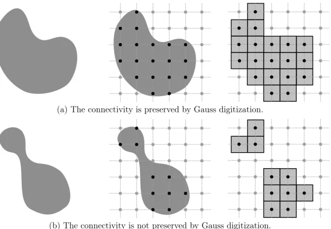
but from an imaging point of view, it can also be seen as a subset of pixels, i.e., unit squares defined as the Voronoi cells of the points of X within R2 (see Fig. 1).
In a recent study about topology-preserving rigid motion of digital objects, we need to compute the Gauss digitization of polygonal objects. More specifically, in Rn, rigid motions
(i.e., transformations based on translations and rotations) are both topology and geometry preserving. Unfortunately, these properties are generally lost in Zn. In [15, 16], a rigid motion
scheme is proposed to allow the preservation of connectivity and some geometric properties (e.g., convexity, area and perimeter) of the transformed digital object. To this end, the proposed scheme relies on (1) a polygonization of the digital object, (2) the transformation of the intermediate piecewise affine object of R2, and (3) a digitization step for recovering
a result within Z2. In this document, we address the step (3) which is to digitize the
transformed polygonal object. Still in [15, 16], if the digital object X is H-convex [11], this digitization process can be done using the polygonal convex hull of X. More precisely, X is defined as the intersection of the smallest set of closed half-plane that include X. In case of non-convex objects, an attempt via the convex decomposition has been considered. This generally works with an extra cost of the decomposition of polygons into convex parts. In this work, we present a method allow to digitize polygons without this decomposition step. The approach is based on the ray casting algorithm for the point-in-polygon problem.
This paper is organized as follows: in section 2 and 3, we recall the basic notions of Gauss digitization and the ray casting algorithm. Section 4 is devoted to formulate the problem of Gauss digitization for simple polygons together with the proposed algorithm for computing the digitized object. Then, in section 5 we present the experimental results. Finally, we conclude the paper with discussion of future works and some applications in section 6.
(a) The connectivity is preserved by Gauss digitization.
(b) The connectivity is not preserved by Gauss digitization.
Figure 1: Left: Continuous object X ⊂ R2. Middle: Gauss digitization of X , X = X ∩ Z2. Right: The digital object X represented by pixels. Due to the resolution of the discrete grid, the Gauss digitization may lead to a disconnection between X and X as shown in the below example.
2
Gauss digitization
Let n ≥ 2. Let X ⊂ Rn be a continuous object. Digitization can be defined as a process
of transforming X into a discrete one, denoted by X. In this work, we consider the Gauss digitization [12], denoted by D, which is simply the intersection of a connected and bounded set X with Zn.
X = X ∩ Zn. (1)
The obtained object is also called a digital object X which is a finite subset of Zn. In 2D and
from an imaging point of view, X ⊂ Z2 can be seen as a subset of unit squares, called pixels,
defined as the Voronoi cells of the points of X (see Fig. 1(a)). Similarly, in 3D, X ⊂ Z3 can
be seen as a subset of the unit cubes, called voxels, whose centers correspond to points of X. Because of this process D, the resulting object may have different properties than those of the original continuous one. An illustration is given Fig. 1(b) in which a connected continuous object X leads, after D, to a disconnected digital object X. In this context, various studies have been proposed for topological preservation of digitized objects under the Gauss digitization D [13, 14, 15, 17, 19, 21, 22]. This is, however, out of scope of the present document. We refer the readers to the cited papers for more details about conditions for topological equivalence of objects by the digitization process D.
(a) (b) (c)
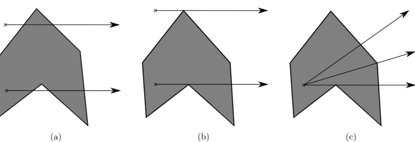
Figure 2: Ray casting algorithm. (a) Simple cases: the rays intersect the polygon edges. (b) Degenerate cases: the rays pass by the polygon vertices which could produce completely incorrect results. (c) Multiple casting rays for handling the degenerate cases. Polygons are in gray and the black polyline is its border, the black arrows are the casting rays.
3
Ray casting algorithm
In this section, we present the main idea of the original ray casting algorithm which will be used for computing the Gauss digitization of polygonal objects.
Point-in-polygon [3, 8], also called point location, is basic problem of computational ge-ometry, and has been considered in many geometry processing applications such as computer vision, computer graphics, geographical information systems, computer aided design, . . .
Roughly speaking, the problem consists in verifying whether a given point in the planes lies inside, outside or on the boundary of a polygonal object. Several solutions have been developed for solving this problem such has triangle tests [2, 4], angle summation test (also called winding number) [6, 9], and crossings test [20, 23].
Among the point-in-polygon algorithms, we are interested in the crossing number test, also known as the even-odd algorithm or the ray casting algorithm. The method is originally proposed by Shimrat in [20]. The idea of this method is to cast a ray from the test point in a fixed direction (the positive x-direction is commonly used), and compute the crossings number –intersection points– of the ray with the polygon edges. The point is on the outside of the polygon if the crossing number is even, and inside otherwise (see Fig. 2(a)).
This method works well whenever the rays intersect the edges only. It may fail if the considered ray passes through the polygon vertices, called the degenerate cases, as illustrated in Fig. 2(b). To tackle this issue, a solution has been presented in [7, 18] by considering that the vertex must be always infinitesimally above the ray. As a consequence, no vertex of the polygon is intersected the ray. Other solution consists in casting multiple rays [5] at the test point, then combining them to provide a solution (see Fig. 2(c)), e.g., via a majority vote. These solutions work in general, but still the parameters –the infinitesimal value, the number of the casting rays and their directions– have to be carefully chosen to avoid other degenerate cases, and not to increase the running time of the whole process.
Hereafter, we present a method for the Gauss digitization of polygonal objects. The method relies on the ray casting algorithm with some modifications allowing to handle the degenerate cases. In particular, it is free-parameter and could be performed in exact calculus.
(a) Simple polygon (b) Self-intersecting polygon (c) Polygon with hole
Figure 3: Examples of polygon: (a) is simple polygon, (b) and (c) are not simple polygons.
4
Gauss digitization for simple polygons
4.1
Problem formulation
Let P be a polygon embedded in R2. We denote δP the boundary of P , also called polyline.
Definition 4.1 A polygon P is called simple, also called Jordan polygon, if its boundary δP form a Jordan curve.
Roughly speaking, simple polygon is a polygon that does not intersect itself and has no hole (see Fig. 3). Such a polygon has a well-defined interior and exterior. Typically, simple polygons are topologically equivalent to a disk.
The point-in-polygon problem can be reformulated as follows: Let P be a simple polygon and p be a point in the plane. The point-in-polygon consists in determining whether p ∈ P . Definition 4.2 Let P ⊂ R2 be a simple polygon. The Gauss digitization of P , denoted by D(P ), is the set of all integer points p ∈ Z2 lies interior to P .
D(P ) = P ∩ Z2 (2)
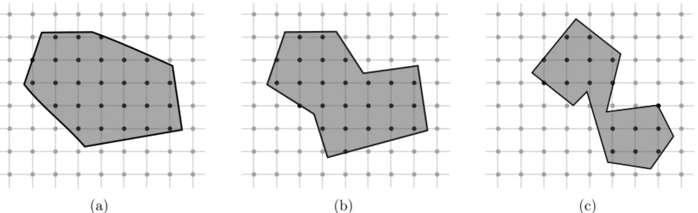
Examples of the Gauss Digitization of simple polygons are given in Fig. 4.
Note that, in order to compute D(P ), it is –impossible and– not necessary to check all points p ∈ Z2 but only those inside the bounding box of δP .
4.2
Proposed algorithm
We slightly modify the ray casting algorithm in the literature in order to handle the degen-erate cases. More precisely, a ray is cast from the test point in a direction such that it hits no vertex of the polyline. A dichotomic search is used to find such a direction. Specifically, we repeat the selection of a direction (e.g., the middle) from two given directions (e.g., the positive x- and y-directions) until we find a direction which does not pass by any vertex of the polyline. The modified ray casting algorithm is given in Algorithm 1, and the whole procedure of the Gauss digitization for simple polygons is summarized in Algorithm 2.
(a) (b) (c)
Figure 4: Gauss digitization of simple polygons: (a) convex polygon, (b) and (c) concave polygons. In (c) the Gauss digitization cause a disconnected digitized set. Polygons are in gray and the black polyline is its border, the black points are the digitized set.
Algorithm 1: Finding a ray that does not pass through any vertex of the polygon
1 Function findDirection
Input: A polygon P = {vi}n1, a point p ∈ Z2, and two points d1, d2for the ray directions
Output: A point d such that the ray pd hits no vertex of P
2 done ← f alse
3 while done = f alse do 4 done ← true
5 d ← (d1+ d2)/2 // Consider the middle point of d1 and d2
6 foreach vi∈ P do
// Verify whether vi lies on the line segment pd
7 if onSegment(p, vi, d) then done ← f alse
8 d2← d
9 return d
Algorithm 2: The Gauss digitization of polygonal objects
1 Algorithm GaussDigitization
Input: A polygon of n vertices P = {vi}n1
Output: The Gauss digitization of P which is P ∩ Z2
2 G ← ∅
// Find the top-left and bottom-right corners of the bounding box of P
3 (tl, br) ←BoundingBox(P ) // tl, br are top-left and bottom-right points 4 for x ← dtl.xe to bbr.xc do
5 for y ← dbr.ye to btl.yc do
6 p ← (x, y) // create point of coordinates (x, y)
7 d1← (p.x, +∞) // a point for the ray from p to the positive x-direction
8 d2← (+∞, p.y) // a point for the ray from p to the positive y-direction
9 d ←findDirection(P, p, d1, d2) // See Algorithm 1
// Check if p is inside or on the border of P (see Algorithm 3)
10 if isInside(P, p, d) = true then
11 G ← G ∪ {p} // If p ∈ P then add p to the set G 12 return G
Algorithm 3: The auxiliary functions used in Algorithm 2
1 Function inInside
Input: A polygon P = {vi}n1, a point p ∈ Z
2and a point d for the ray direction
Output: Boolean indicating whether p lies inside or on the border of P
2 if n < 3 then return f alse 3 i ← 0
4 count ← 0 5 do
6 next ← (i + 1) % n
// Check if the ray pd intersects the edge vi, vnext of P
7 if doIntersect(p, d, vi, vnext) = true then
// Check if p is on the edge vi, vnext of P
8 if onSegment(vi, p, vnext) = true then return true
9 else return f alse 10 count ← count + 1 11 while i 6= 0
12 return count % 2 = 1 // Return true if count is odd, false otherwise 13 Function onSegment
Input: Three points p,q and r
Output: Boolean indicating whether p lies on the line segment pr // Check if p is colinear with the line segment pr
14 if orientation(vi, p, vnext) = 0 then
15 if (q.x ≤ max(p.x, r.x)&q.x ≥ min(p.x, r.x)&q.y ≤ max(p.y, r.y)&q.y ≥ min(p.y, r.y)) then 16 return true
17 return false 18 Function orientation
Input: Three points p,q and r
Output: A value indication the orientation of ordered triplet (p, q, r)
19 v ← (q.y − p.y) ∗ (r.x − q.x) − (q.x − p.x) ∗ (r.y − q.y) 20 if v = 0 then
21 return 0 // three point are colinear
22 return (val > 0) ? 1 : 2 // 1 if clockwise and 2 for counterclockwise orientation 23 Function doIntersect
Input: Four points p1, q1, p2 and q2
Output: Boolean indicating whether the line segment p1q1 intersects the line segment p1q1
24 o1← orientation (p1, q1, p2) 25 o2← orientation (p1, q1, q2) 26 o3← orientation (p2, q2, p1)
27 o4← orientation (p2, q2, q1)
// Two segments p1q1 and p1q1 intersect
28 if (o16= o2 & o36= o4) then return true;
// p1, q1 and p2 are colinear and p2 lies on segment p1q1
29 if (o1= 0 & onSegment(p1, p2, q1)) = true then return true
// p1, q1 and p2 are colinear and q2 lies on segment p1q1
30 if (o2= 0 & onSegment(p1, q2, q1)) = true then return true
// p2, q2 and p1 are colinear and p1 lies on segment p2q2
31 if (o3= 0 & onSegment(p2, p1, q2)) = true then return true
// p2, q2 and p1 are colinear and q1 lies on segment p2q2
32 if (o4= 0 & onSegment(p2, q1, q2)) = true then return true
In particular, if the input polygon has integer / rational coordinates, then the proposed procedure works in exact computation (and thus without numerical errors).
Complexity analysis: For a given point p and a simple polygon P , the verification of p ∈ P costs O(n log n) [10] for n is the number of polygon vertices. The dichotomic search is also O(n log n). Therefore, the overall complexity of the Gauss digitization of P is O(mn log n) for m is the size of the bounding box of P .
Implementation: The method is implemented in C++ and uses Dgtal library [1] to output images. Note that this implementation is based on the solution given at https:// www.geeksforgeeks.org/how-to-check-if-a-given-point-lies-inside-a-polygon/ with the modification explained previously. The code is available at:
https://github.com/ngophuc/GaussDigitization
5
Experiments
Some experimental results of the Gauss digitization of polygonal objects are given in Fig. 5. Three different ray-casting methods are perform for the experiments:
• The first one is to use only on ray from the test point in the positive x-direction, and report the result according to the crossing numbers.
• The second is to use two rays from the test point in the positive x- and y-directions, and reports the result if at least one of the ray satisfies the crossing numbers.
• The third one is the proposed method which first finds the ray hitting no vertex of the polygon, then reports the result of the ray according to its crossing numbers.
On can observe that the results obtained by the first two methods are incorrect and contain many artifacts related to the ray casting directions. Indeed, it is mainly caused by the degenerate cases, as explained in Sec. 3. With the proposed modification of the ray casting method, we obtain a much better and correct results.
6
Conclusion
In this paper we presented a modified version of ray casting algorithm to handle the degen-erate cases. The method is used to compute the Gauss digitization of simple polygons. The method is very simple and easy to implement. It has a complexity of O(mn log n) for n is the number of polygon vertices and m is the size of the bounding box of the polygon. This algorithm could be used in [15, 16] for topology-preserving rigid motion of digital objects.
In future works, we would like to extend the method into 3D for the polyhedra and to integrate the code to the Dgtal library [1].
Figure 5: Gauss digitization of polygonal objects using ray casting algorithm. Left: Results obtained by using 1 ray in the positive x-direction. Middle: Results obtained by using 2 rays in the positive x- and y-directions. Right: Results obtained by the modified ray casting algorithm. The input polylines are in red, and the grey pixels are the digitized objects.
References
[1] DGtal: Digital Geometry tools and algorithms library, http://libdgtal.org
[2] Badouel, D.: An Efficient Ray-Polygon Intersection, p. 390–393. Academic Press Pro-fessional, Inc., USA (1990)
[3] Berg, M.d., Cheong, O., Kreveld, M.v., Overmars, M.: Computational Geometry: Al-gorithms and Applications. Springer-Verlag TELOS, Santa Clara, CA, USA, 3rd ed. edn. (2008)
[4] Berlin, J.E.P.: Efficiency considerations in image synthesis 11 (1985)
[5] Brecheisen, R., Vilanova, A., Platel, B., Romeny, B.T.H.: Flexible gpu-based multi-volume ray-casting. In: VMV (2008)
[6] Gatilov, S.: Efficient angle summation algorithm for point inclusion test and its robust-ness. Reliab. Comput. 19, 1–25 (2013)
[7] Glassner, A.S. (ed.): An Introduction to Ray Tracing. Academic Press Ltd., GBR (1989) [8] Haines, E.: Point in Polygon Strategies, p. 24–46. Academic Press Professional, Inc.,
USA (1994)
[9] Hormann, K., Agathos, A.: The point in polygon problem for arbitrary polygons. Com-put. Geom. Theory Appl. 20(3), 131–144 (Nov 2001). https://doi.org/10.1016/S0925-7721(01)00012-8
[10] Huang, C.W., Shih, T.Y.: On the complexity of point-in-polygon algorithms. Computers & Geosciences 23(1), 109 – 118 (1997). https://doi.org/https://doi.org/10.1016/S0098-3004(96)00071-4
[11] Kim, C.E.: On the cellular convexity of complexes. IEEE Transactions on Pattern Analysis and Machine Intelligence PAMI-3(6), 617–625 (1981)
[12] Klette, R., Rosenfeld, A.: Digital Geometry: Geometric Methods for Digital Picture Analysis. Elsevier, Amsterdam, Boston (2004)
[13] Latecki, L.J., Conrad, C., Gross, A.: Preserving topology by a digitization process. Journal of Mathematical Imaging and Vision 8(2), 131–159 (1998)
[14] Ngo, P., Passat, N., Kenmochi, Y., Debled-Rennesson, I.: Convexity in-variance of voxel objects under rigid motions. In: International Confer-ence on Pattern Recognition (ICPR), Proceedings. pp. 1157–1162 (2018). https://doi.org/10.1109/ICPR.2018.8545023
[15] Ngo, P., Passat, N., Kenmochi, Y., Debled-Rennesson, I.: Geometric preservation of 2D digital objects under rigid motions. Journal of Mathematical Imaging and Vision 61(2), 204–223 (2019). https://doi.org/10.1007/s10851-018-0842-9
[16] Ngo, P., Kenmochi, Y., Passat, N., Debled-Rennesson, I.: Discrete regular polygons for digital shape rigid motion via polygonization. In: Reproducible Research in Pattern Recognition. pp. 55–70. Springer International Publishing (2019)
[17] Pavlidis, T.: Algorithms for Graphics and Image Processing. Berlin: Springer, and Rockville: Computer Science Press (1982)
[18] Preparata, F.P., Shamos, M.I.: Springer New York, New York, NY (1985). https://doi.org/10.1007/978-1-4612-1098-6_1
[19] Serra, J.: Image Analysis and Mathematical Morphology. Academic Press, Inc., Or-lando, FL, USA (1983)
[20] Shimrat, M.: Algorithm 112: Position of point relative to polygon. Commun. ACM 5(8), 434 (Aug 1962). https://doi.org/10.1145/368637.368653
[21] Stelldinger, P., Köthe, U.: Towards a general sampling theory for shape preservation. Image and Vision Computing 23(2), 237–248 (2005). https://doi.org/10.1016/j.imavis.2004.06.003
[22] Stelldinger, P., Terzic, K.: Digitization of non-regular shapes in arbi-trary dimensions. Image and Vision Computing 26(10), 1338–1346 (2008). https://doi.org/10.1016/j.imavis.2007.07.013
[23] Vandewettering, M., Haines, E., Kalenda, E.J., Parent, R., Uselton, S., Andersson, Z., Holloway, B.: Point in polygon, one more time... Ray Tracing News 3(4) (1990)