HAL Id: hal-01878722
https://hal.archives-ouvertes.fr/hal-01878722
Submitted on 21 Sep 2018
HAL is a multi-disciplinary open access
archive for the deposit and dissemination of
sci-entific research documents, whether they are
pub-lished or not. The documents may come from
teaching and research institutions in France or
abroad, or from public or private research centers.
L’archive ouverte pluridisciplinaire HAL, est
destinée au dépôt et à la diffusion de documents
scientifiques de niveau recherche, publiés ou non,
émanant des établissements d’enseignement et de
recherche français ou étrangers, des laboratoires
publics ou privés.
Experimental Characterization of Cohesive Zone Models
for Thin Adhesive Layers Loaded in Mode I, Mode II,
and Mixed-Mode I/II by the use of a Direct Method
G. Lélias, Eric Paroissien, Frederic Lachaud, Joseph Morlier
To cite this version:
G. Lélias, Eric Paroissien, Frederic Lachaud, Joseph Morlier. Experimental Characterization of
Co-hesive Zone Models for Thin AdCo-hesive Layers Loaded in Mode I, Mode II, and Mixed-Mode I/II
by the use of a Direct Method.
International Journal of Solids and Structures, Elsevier, 2019,
�10.1016/j.ijsolstr.2018.09.005�. �hal-01878722�
1
Experimental Characterization of Cohesive Zone Models for Thin Adhesive Layers
1
Loaded in Mode I, Mode II, and Mixed-Mode I/II by the use of a Direct Method
2
3
4
5
G. Lélias1,2, E. Paroissien1,*, F. Lachaud1 and J. Morlier1
6
7
8
1Institut Clément Ader (ICA), Université de Toulouse, UPS, INSA, ISAE-SUPAERO, MINES-ALBI, CNRS, 3 rue
9
Caroline Aigle, 31400 Toulouse, France
10
2 SOGETI HIGH TECH, AEROPARK, 3 Chemin Laporte, 31300 Toulouse, France
11
12
13
14
15
16
17
18
19
20
21
*To whom correspondence should be addressed: Tel. +33561338438, E-mail: eric.paroissien@isae-supaero.fr
22
23
24
25
26
27
28
2
1
Abstract – The demand for designing lightweight structures without any loss of strength or stiffness has
2
conducted many engineers and researchers to seek for alternative joining methods. In this context, adhesive
3
bonding may appear as an attractive joining method. However the interest of adhesive bonding remains while the
4
structural integrity of the joint is ensured. According to recent literature the Cohesive Zone Model (CZM)
5
appears as a suitable approach able to predict both static and fatigue strength of adhesively bonded joints. This
6
approach of the fracture process of adhesive layers is based on the modeling of the adhesive mechanical behavior
7
through a set of adhesive cohesive properties in either mode I, mode II or mixed-mode I/II. The strength
8
prediction of adhesively bonded joints is then highly dependent on the CZM parameters. The methods used to
9
experimentally characterize them are thus essential. A new methodology, termed direct method, is presented and
10
tested. It is based on the measurement of displacement field of bonded adherends at the crack tip of classical
11
specimens allowing for the loading of the adhesive layer in pure mode I, pure mode II and mixed-mode I/II. The
12
tested adhesive is a methacrylate–based two-component adhesive paste found under the reference SAF30 MIB
13
manufactured by AEC Polymers (ARKEMA group). The adherends are in aluminium 6060. It is shown that it is
14
possible to characterize the cohesive properties of the adhesive layer using the direct method. The numerical
15
tests involve both adherends and adhesive nonlinearities. Nevertheless, the presented experimental
16
implementation passes by the development of a dedicated data pre-processing to interpret the experimental
17
measurements, highlighting the significance of the choice of the measurement means linked to the design of
18
specimen.
19
20
21
Key words: adhesively bonded joint, cohesive zone model, macro-element, mode I, mode II, mixed-mode I/II,
22
singular value decomposition, digital image correlation technique
23
3
NOMENCALTURE AND UNITS1
BBe bonded-beams element
2
CZM cohesive zone model
3
DIC digital image correlation
4
DoE design of experiments
5
DCB double cantilever beam
6
ENF end notched flexure
7
FE Finite Element
8
ME macro-element
9
MMB mixed mode bending
10
OSRA optimal sub rank approximation
11
SLJ single-lap joint
12
SVD singular value decomposition
13
Aj extensional stiffness (N) of adherend j
14
Bj extensional and bending coupling stiffness (N.mm) of adherend j
15
Dj bending stiffness (N.mm2) of adherend j
16
E adherend Young’s modulus (MPa)
17
GI strain energy release rate (energy per unit of area: mJ or N/mm) in peel
18
GII strain energy release rate (energy per unit of area: mJ or N/mm)in shear
19
GIc critical strain energy release rate (energy per unit of area: mJ or N/mm)in peel
20
GIe adhesive elastic strain energy stored (energy per unit of area: mJ or N/mm)in peel
21
GIIc critical strain energy release rate (energy per unit of area: mJ or N/mm)in shear
22
GIIe adhesive elastic strain energy stored (energy per unit of area: mJ or N/mm)in shear
23
H magnitude of applied displacement (mm)
24
J J-integral parameter
25
KBBe elementary stiffness matrix of a bonded-beam element
26
L length (mm) of bonded overlap
27
Mj bending moment (N.mm) in adherend j around the z direction
28
Nj normal force (N) in adherend j in the x direction
29
P magnitude of applied force (N)
4
S adhesive peel stress (MPa)1
Smax maximal adhesive peel stress (MPa)
2
T adhesive shear stress (MPa)
3
Tmax maximal adhesive shear stress (MPa)
4
Vj shear force (N) in adherend j in the y direction
5
a crack length (mm)
6
b width (mm) of the adherends
7
d damage parameter
8
e thickness (mm) of the adhesive layer
9
hj half thickness (mm) of adherend j
10
kI adhesive elastic stiffness (MPa/mm) in peel
11
kII adhesive elastic stiffness (MPa/mm) in shear
12
n power usd in the adhesive material law
13
n_ME number of macro-elements
14
t adherend thickness (mm)
15
uj displacement (mm) of adherend j in the x direction
16
vj displacement (mm) of adherend j in the y direction
17
overlap length (mm) of a macro-element
18
j characteristic parameter of adherend j in N2.mm2
19
angle (rad) used for the definition the load application in MCB test
20
mixed-mode parameter
21
t numerical time step (s)
22
u displacement jump (mm) of the interface along the x-axis
23
ue displacement jump (mm) of the interface along the x-axis at initiation
24
uf displacement jump (mm) of the interface along the x-axis at propagation
25
v displacement jump (mm) of the interface along the y-axis
26
ve displacement jump (mm) of the interface along the x-axis at initiation
27
vf displacement jump (mm) of the interface along the x-axis at propagation
28
norm of displacement jump (mm) of the interface
29
e norm of displacement jump (mm) of the interface at initiation
5
f norm of displacement jump (mm) of the interface at propagation1
adherend Poisson’s ratio
2
j bending angle (rad) of the adherend j around the z direction
3
4
1. Introduction
5
In the frame of structural design, the choice of joining technologies is decisive since they guarantee the integrity
6
of the manufactured system. The mechanical fastening, such as riveting or screwing, appears the reliable solution
7
for the designers. Nevertheless alone or in combination with the mechanical fastening, the adhesive bonding
8
joining technology may offer significantly improved mechanical performance in terms of stiffness, static
9
strength and fatigue strength (Hart-Smith 1980, Kelly 2006). The use of this higher level of mechanical
10
performance allows for the design of lighter joints. In other words, the adhesive bonding offers the possibility to
11
reduce the structural mass while ensuring the mechanical strength. The optimization of the strength-to-mass ratio
12
is a challenge for several industrial sectors, such as aerospace, automotive, rail or naval transport industries. But,
13
the reduction of structural mass makes sense only if the structural integrity is ensured. As result to take benefit
14
from the adhesive bonding in view of mass reduction, it is required to be able to predict the strength of bonded
15
joints. The strength prediction consists in the comparison of computed strength criteria to design allowable
16
value. The strength criteria could be based on theoretical, empirical, semi-empirical investigations and possibly
17
including in-service feedback. The stress analysis allows for the computation of input data, mandatory to the
18
assessment of strength criteria. The experimental characterization allows then for the definition of design
19
allowable value as well as of mechanical behavior to be used as input data of the mechanical analysis. As
20
highlighted in (Jumel et al. 2013), the strength of a same joining system at macroscale depends on the
21
experimental test specimen and procedure used, which contributes in restricted reliability or in extensive and
22
expensive experimental test campaign. According to (Li et al. 2006, Khoramishad et al. 2010, Khoramishad et
23
al. 2011, Da Silva and Campilho 2012), the cohesive zone modeling – denoted CZM – appears as one of the
24
most suitable approach able to model both the static and the fatigue behavior of adhesive joints. According to
25
(Khoramishad et al. 2010), the CZM have the advantage of: (i) considering finite strains and stresses at the
26
adhesive crack tip, (ii) indicating both damage initiation and propagation as direct outputs of the model, (iii)
27
advancing the crack tip as soon as the local energy release rate reaches its critical value with no need of complex
28
moving mesh techniques. Based on Continuum Damage Mechanics and Fracture Mechanics, the CZM enables a
29
diagnostic of the current state of the adhesive interface damage along the overlap. The damage, associated to
6
micro-cracks and/or voids coalescence, results in a progressive degradation of the material stiffness before
1
failure. An idealization of a CZM bilinear stress-strain relationship or CZM bilinear traction separation law is
2
presented in Figure 1. The CZM bilinear traction separation law is a well-established interface behavior that first
3
assumes a linearly dependency relationship between the interface separation (deformation) and the resulting
4
traction (stress). Once a prescribed value of separation is reached by the adhesive, the damage initiation is
5
described in the form of a linearly decreasing resulting traction. Finally, the propagation of the damage is
6
described by voluntarily fixing the resulting traction to zero, hence modeling the creation of two traction-free
7
surfaces (i.e.: physical cracking). Both damage initiation and damage propagation phases are addressed in the
8
model with no need of assuming any initial crack in the material (Valoroso and Champaney 2004, De Moura et
9
al. 2009, Campilho et al. 2013).
10
11
Figure 1. Representation for an idealized bilinear interface traction separation law.
12
13
The strength prediction of adhesively bonded joints is then highly dependent on the CZM parameters. The
14
methods used to experimentally characterize them are thus essential. As a result, numbers of authors have
15
addressed this critical point over the past few years (Anderson and Stigh 2004, Alfredsson et al. 2003,
16
Alfredsson 2004, Leffler et al. 2006, Högberg 2006, Högberg and Stigh 2006, Cui et al. 2014, Azari et al. 2009,
17
Gowrishankar S. et al. 2012, Wu et al. 2016). Most of these methods make use of the concept of the energetical
18
balance associated to the computation of the path independent J-integral (Rice 1968) along a closed contour of
19
specifically designed joint specimens, known as the inverse method (Anderson and Stigh 2004, Alfredsson et al.
20
2003, Alfredsson 2004, Leffler et al. 2006, Högberg 2006, Högberg and Stigh 2006). The inverse method is
21
δ δf δe : Fracture energy : ks=(1-d)*k(unloading) σ(δe)=kδe : k (loading) Idealized bilinear interfacetraction separation law: Initiation of the damage
Propagation of the damage
7
based on the energetical balance associated with the computation of the path independent J-integral (Rice 1968)
1
on a closed contour :
2
𝐽 = ∫ 𝑊𝑑𝑦 − 𝑇̅𝑑𝑈̅𝑑𝑥𝑑𝑠 (1)
3
where W refers to the strain energy density,
T
n
to the traction vector, σ to the stress tensor, 𝑈̅ to the4
displacement vector, n to the normal unit vector directed outward to the counter-clock wise integration path Γ,
5
and (x,y) to the specified two-dimensional coordinate system. From the fundamental work by (Fraisse and
6
Schmit 1993) it is shown that the J-integral parameter can be computed from stress analysis based on a model of
7
beam on an elastic foundation as:
8
𝐽(𝛿𝑢, 𝛿𝑣) = ∫ 𝑇(𝛿𝑢, 𝛿𝑣)𝑑𝛿𝑢 𝛿𝑢 0 + ∫ 𝑆(𝛿𝑢, 𝛿𝑣)𝑑𝛿𝑣 𝛿𝑣 0 (2)9
In the frame of the inverse method:
10
(i) the adhesive peel stress is obtained from experimental tests under pure mode I loading as (Anderson and Stigh
11
2004):12
𝑆(𝛿𝑣) =𝜕𝐽(𝛿𝑢,𝛿𝑣 ) 𝜕𝛿𝑣 (3)13
(ii) the adhesive shear stress is obtained from experimental tests under pure mode II loading as (Alfredsson et al.
14
2003):15
𝑇(𝛿𝑢) =𝜕𝐽(𝛿𝜕𝛿𝑢,𝛿𝑣) 𝑢 (4)16
(iii) the adhesive peel and shear stresses are obtained from experimental tests under mixed-mode I/II loading as
17
(Högberg 2006, Högberg and Stigh 2006):
18
𝑆(𝛿𝑣) =𝜕𝐽(𝛿𝜕𝛿𝑢,𝛿𝑣) 𝑣 (5)19
𝑇(𝛿𝑢) =𝜕𝐽(𝛿𝜕𝛿𝑢,𝛿𝑣) 𝑢 (6)20
The adhesive stresses are then derived from the J-integral. An advantage of this method is that it offers the
21
possibility to monitor the evolution of the adhesive stress at the crack tip from the measurement of macroscopic
22
quantities possibly measurable from experimental test fixtures, such as the applied load (in N) or the evolution of
23
displacement jump (in mm) at the crack tip. Numbers of joint specimens have been explored for pure mode I,
24
pure mode II and mixed-mode I/II characterization of adhesive layers. According to (Da Silva and Campilho
25
2012), end notched flexure (ENF) and double cantilever beam (DCB) joint specimens have respectively emerged
26
as the joint specimens the most frequently used for characterizing the cohesive properties of thin adhesive
27
interfaces in pure mode I and pure mode II over the past years. An idealization of the linear elastic distributions
8
of adhesive stresses (strains) resulting from the loading of both ENF and DCB joint specimens is presented in
1
Figure 2. According to (Reeder and Crews 1990, Kenane and Benzeggagh 1997, Högberg 2006) most of the
2
mixed-mode I/II test fixture present practical limitations: (i) complex loading fixtures, (ii) unstable fracture
3
process, (iii) complex manufacturing of the test samples. However, both mixed mode cantilever beam (MCB)
4
and mixed mode bending (MMB) joint specimens offer the possibility of working over a wide range of adhesive
5
mixed-mode ratios without modifying the geometry (Figure 2).
6
7
8
Figure 2. Schematic representation for the (a) End Notched Flexure (ENF), (b) Double Cantilever Beam (DCB)
9
adhesive joint specimens. Idealized adhesive stress distributions, (c) Mixed-mode Cantilever Beam (MCB) and
10
(d) Mixed-Mode Bending (MMB) adhesive joint specimens.
11
12
However, the methods based on J-integral are valid only when the J-integral is valid. If the J-integral can be
13
computed through a data reduction scheme based on a model of a beam on elastic foundations for the adhesive
14
bonded overlap (Fraisse and Schmit 1993), the J-integral is not suitable when the materials are dependent on
15
time. Another restriction is the consideration of unloading phases within the loading history. Various types of
16
CZM for mixed-mode exist in the literature (Goustanios and Sørensen 2012). One widespread type is based on
17
the definition of traction-separation laws in pure modes, which are coupled with interaction laws for damage
18
initiation and damage propagation under mixed-mode. Goustanios and Sørensen show that the mixed-mode
19
truss-like CZMs are path-dependent. The mixed-mode truss-like CZMs are a particular case of mixed-mode
20
CZM based on the definition of pure modes laws linked by interaction laws under mixed-mode. If the J-integral
21
t P a ENF e L t b = width (a) t P P a L DCB e t (b) L MCB e t P P
t (c) P a (d) MMB e t c t L9
is path-independent along the spatial integration path, it is shown that the J-integral, which is shown to be a
1
potential function from which derive the cohesive stress, is dependent on the loading path history. A direct
2
consequence for truss-like CZMs is thus that Eq. (2) does not imply Eq. (5) and Eq. (6), so that the use of the
3
inverse method should not be suitable to any type of CZM.
4
The objective of this paper is to suggest a direct method to assess CZMs for the modelling of adhesively bonded
5
joints, overcoming the restrictions involved in methods based on J-integral. In the first part, the inverse method
6
is employed on the results of a numerical test campaigns on MCB configuration. A mixed-mode CZM based on
7
the definition of pure mode bilinear laws linked by interaction laws under mixed-mode is used for this test
8
campaign in order to show the deviation of predictions obtained from the inverse method. The numerical
9
analyses are performed using three-dimensional Finite Element (3D FE) model as well as the macro-element
10
(ME) technique (Paroissien 2006a, Paroissien et al. 2006b, Paroissien et al. 2007, Paroissien et al. 2013, Lélias
11
et al. 2015). In the second part, an approach based on design of experiments (DoE) is presented to assess the
12
main parameters affecting the experimental assessment of CZM. Finally, in the part, the direct method is applied
13
to characterize the CZM properties in mode I, mode II and mixed-mode I/II through the use of double cantilever
14
beam (DCB) specimen, end notched flexure (ENF) specimen and mixed mode bending (MMB) specimen,
15
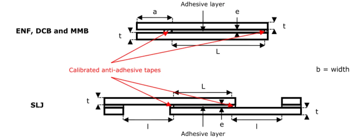
respectively (see Figure 3). Finally the single-lap bonded joint (SLJ) configuration is used to assess the relevance
16
of the method (see Figure 3).
17
18
Figure 3. Schematic representation for the manufacturing process of the ENF, DCB, MMB and SLJ joint
19
specimens.
20
21
2. Numerical test campaign
22
2.1. Overview of the numerical test campaign
23
a
L
ENF, DCB and MMB
SLJ
Calibrated anti-adhesive tapes
L l l Adhesive layer Adhesive layer t t t t e e b = width
10
In the frame of the numerical test campaign presented in this paper, the MCB test configuration has been
1
selected. It has been suggested by Högberg and Stigh (Högberg and Stigh 2006). Similarly to the DCB test
2
configuration, the loading consists in a pair of forces (termed P), being of the same magnitude but in opposite
3
directions. Nevertheless, the action direction of the pair of forces is defined by an angle , which allows for the
4
adhesive layer to be submitted to pure mode I, pure mode II and mixed-mode I/II (see Figure 2). The selected
5
specimen design, including geometrical and material parameters, corresponds to the one described by Högberg
6
and Stigh (Högberg and Stigh 2006). The crack length a=0 is then chosen. The geometrical parameters are
7
provided in Table 1 in conjunction with Figure 2. In this numerical test campaign, only one angle is chosen
8
/16.
9
10
Table 1. Geometrical parameters of the MCB specimen.
11
a in mm b in mm e in mm t in mm L in mm
0 4 0.2 8 100
12
The adherends are made of steel with a Young’s modulus E=200 GPa and a Poisson’s ratio =0.3. The design is
13
such that the adherends will remain in their linear elastic domain. The adhesive is assumed to have a classical
14
bilinear damage evolution law following (Allix and Ladevèze 1996), involving interaction energy laws for both
15
initiation and propagation under mixed-mode:
16
{( 𝐺𝐼 𝐺𝐼𝑒) 𝑛 + (𝐺𝐼𝐼 𝐺𝐼𝐼𝑒) 𝑛 = 1 (𝐺𝐼 𝐺𝐼𝑐) 𝑚 + (𝐺𝐼𝐼 𝐺𝐼𝐼𝑐) 𝑚 = 1 (7)17
where n=m is a material parameter to be identified, GIc and GIIc are the critical strain energy release ratein mode
18
I and mode II, GIe and GIIe are the elastic strain energies stored in mode I and mode II and GI and GII are related
19
to the strain energy release rates in mode I and mode II, respectively. For this numerical test campaign, n=1 is
20
chosen. The fracture energies in mode I and mode II and the elastic stiffnesses under peel and shear, termed kI
21
and kII respectively are the same as those used by Högberg and Stigh (Högberg and Stigh 2006). Nevertheless,
22
the adhesive maximal peel and shear stresses, termed Smax and Tmax, is different, to ensure a right energy
23
dissipation during loading (Turon et al. 2010). It is indicated that the law by Allix and Ladevèze (Allix and
24
Ladevèze 1996) already includes this condition. It is then chosen to keep the same maximal shear stress Tmax=26
25
MPa, resulting in a maximal peel stress Smax=36.6 MPa, instead of 20 MPa. The choice consisting in keeping
26
Smax to its original value instead of Tmax does not change qualitatively the results provided in his paper. The
11
material parameters of the adhesive layer are given in Table 2. In the following, the 3D FE model and the ME
1
model are presented. Then the results of the numerical test campaign are provided including those relating to the
2
convergence study of numerical models. Finally, the direct method is described.
3
4
Table 2. Adhesive material parameters.
5
GIc in N/mm GIe in N/mm GIIe in N/mm GIIc in N/mm
0.76 3.128 E-2 3.464 E-2 2.30
ve in mm vf in mm ue in mm uf in mm
1.71 E-3 4.15 E-2 7.28 E-3 1.77 E-1
kI in GPa/mm Smax in MPa kII in GPa/mm Tmax in MPa
21.4 36.6 3.57 26
6
2.2. Macro-element model
7
Macro-element technique. The numerical analysis is performed using the ME technique for the modelling of
8
bonded overlap (Paroissien 2006a, Paroissien et al. 2006b, Parossien et al. 2007, Paroissien et al. 2013, Lélias et
9
al. 2015). The ME technique is inspired by the FE method and differs in the sense that the interpolation functions
10
are not assumed, since they take the shape of the solutions of the governing differential equation system. A direct
11
consequence is that only one ME is sufficient to mesh a complete bonded overlap in the frame of a linear stress
12
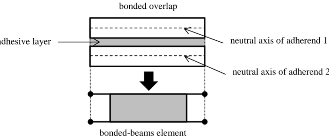
analysis. The bonded overlap is then modelled by a four-node ME – also called bonded-beams element – the
13
nodes of which are located at the extremities of the overlap on the neutral axes of adherends (see Figure 4). This
14
ME involves 3 degrees of freedom per node or a total of twelve for a 1D-beam analysis.
15
16
stress displacement jump mode I kI GIe GIc Smax ve vf stress displacement jump mode II kII GIIc Tmax ue uf GIIe12
1
Figure 4. Modelling of a bonded overlap by a bonded-beams element.
2
3
The main work is thus the formulation of the elementary stiffness matrix of the bonded-beams element. Indeed
4
once the stiffness matrix of the complete structure is assembled from the elementary matrices and the boundary
5
conditions are applied, the minimization of the potential energy provides the solution, in terms of distributions
6
along the overlap of adhesives stresses, internal forces and displacements in the adherends. An approach for the
7
formulation of the stiffness has already been described in detail in previous papers (Paroissien 2006a, Paroissien
8
et al. 2006b, Paroissien et al. 2007, Paroissien et al. 2013, Lélias et al. 2015). Nevertheless, this approach could
9
be long to set up. In this paper, a new approach is provided in Appendix A for a fast and easy implementation
10
within a mathematical software such as SCILAB for example. Compared with the early approach, the shape of
11
solutions in terms of displacements and internal loads is not provided. Nevertheless, in the frame of nonlinear
12
material analyses such as the one presented in this paper, the bonded overlap has to be meshed in order to locally
13
update the material parameters within an iterative computation procedure. As a result, the displacements and
14
internal loads are directly read at nodes. Moreover, the following description is useful for the derivation of the
15
direct method.
16
Hypotheses. It is assumed that the thickness of the adhesive is constant along the length of the macro-element.
17
Moreover, the adherends are simulated as linear elastic Euler-Bernoulli laminated beams. The general shape of
18
the constitutive equations for the adherend j=1,2 provides the six first differential equations:
19
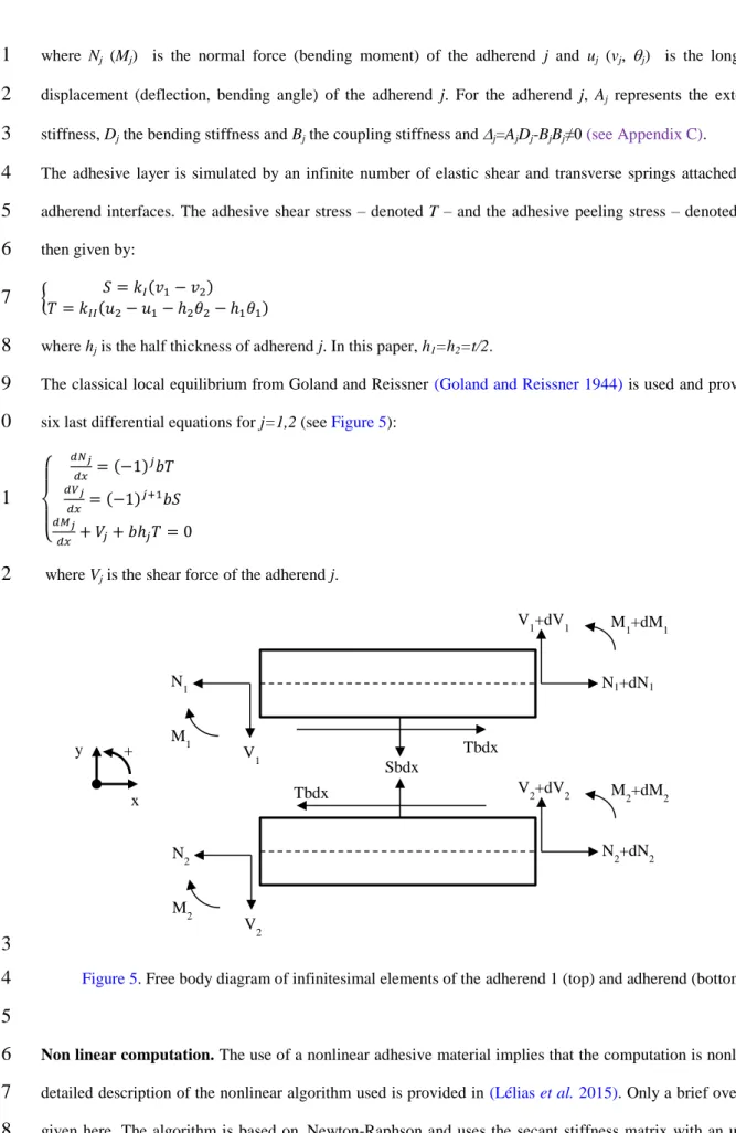
{ 𝑁𝑗= 𝐴𝑗 𝑑𝑢𝑗 𝑑𝑥 − 𝐵𝑗 𝑑𝜃𝑗 𝑑𝑥 𝑀𝑗= −𝐵𝑗 𝑑𝑢𝑗 𝑑𝑥 + 𝐷𝑗 𝑑𝜃𝑗 𝑑𝑥 𝜃𝑗= 𝑑𝑣𝑗 𝑑𝑥 ⇔ { 𝑑𝑢𝑗 𝑑𝑥 = 𝐷𝑗 Δ𝑗𝑁𝑗+ 𝐵𝑗 Δ𝑗𝑀𝑗 𝑑𝑣𝑗 𝑑𝑥 = 𝜃𝑗 𝑑𝜃𝑗 𝑑𝑥 = 𝐵𝑗 Δ𝑗𝑁𝑗+ 𝐴𝑗 Δ𝑗𝑀𝑗 (8)20
bonded overlap bonded-beams elementneutral axis of adherend 1
neutral axis of adherend 2 adhesive layer
13
where Nj (Mj) is the normal force (bending moment) of the adherend j and uj (vj, j) is the longitudinal
1
displacement (deflection, bending angle) of the adherend j. For the adherend j, Aj represents the extensional
2
stiffness, Dj the bending stiffness and Bj the coupling stiffness and j=AjDj-BjBj≠0 (see Appendix C).
3
The adhesive layer is simulated by an infinite number of elastic shear and transverse springs attached at both
4
adherend interfaces. The adhesive shear stress – denoted T – and the adhesive peeling stress – denoted S – are
5
then given by:
6
{𝑇 = 𝑘 𝑆 = 𝑘𝐼(𝑣1− 𝑣2)
𝐼𝐼(𝑢2− 𝑢1− ℎ2𝜃2− ℎ1𝜃1) (9)
7
where hj is the half thickness of adherend j. In this paper, h1=h2=t/2.
8
The classical local equilibrium from Goland and Reissner (Goland and Reissner 1944) is used and provides the
9
six last differential equations for j=1,2 (see Figure 5):
10
{ 𝑑𝑁𝑗 𝑑𝑥 = (−1) 𝑗𝑏𝑇 𝑑𝑉𝑗 𝑑𝑥 = (−1) 𝑗+1𝑏𝑆 𝑑𝑀𝑗 𝑑𝑥 + 𝑉𝑗+ 𝑏ℎ𝑗𝑇 = 0 (10)11
where Vj is the shear force of the adherend j.
12
13
Figure 5. Free body diagram of infinitesimal elements of the adherend 1 (top) and adherend (bottom)
14
15
Non linear computation. The use of a nonlinear adhesive material implies that the computation is nonlinear. A
16
detailed description of the nonlinear algorithm used is provided in (Lélias et al. 2015). Only a brief overview is
17
given here. The algorithm is based on Newton-Raphson and uses the secant stiffness matrix with an update at
18
Sbdx Tbdx Tbdx N1+dN1 V 1+dV1 M1+dM1 N2+dN2 V2+dV2 M2+dM2 N 1 V1 M1 N 2 V2 M2 x y +14
each iteration. In particular, the damage parameter is computed at each nodal abscissa according to the
1
introduced adhesive material law. The norm of displacement jump (in mm) of interface is defined by:
2
𝜆 = √(𝛿𝑣)2+ (𝛿𝑢)2 (11)
3
where v (u) is the displacement jump of the interface (see Table 2) along the y-axis (x-axis). A mixity
4
parameter is defined by:
5
𝛽 =𝛿𝑢 𝛿𝑣= 𝑢2−𝑢1−ℎ2𝜃2−ℎ1𝜃1 𝑣1−𝑣2 (12)6
At each iteration, the mixity parameter is updated. Under the current local mixity parameter, it assumed that
7
the material law is bilinear, so that the damage parameter d is such that:
8
𝑑 =𝜆𝑓(𝜆−𝜆𝑒)
𝜆(𝜆𝑓−𝜆𝑒) (13)
9
where e (f) is the displacement jump (in mm) of the interface at initiation (propagation). In order to compute e
10
(f), the interaction laws Eq. (1) are used while classically assuming that the projections on pure modes of the
11
mixed mode evolution law under the current local mixity are bilinear (see Table 2):
12
{ 𝜆𝑒= 𝛿𝑢𝑒𝛿𝑣𝑒√1 + 𝛽2[(𝛿 1 𝑢𝑒)2𝑛+(𝛽𝛿𝑣𝑒)2𝑛] 1 2𝑛 𝜆𝑓 = 𝛿𝑢𝑓𝛿𝑣𝑓√1 + 𝛽2[ √(𝛿𝑢𝑒 )2𝑛+(𝛽𝛿𝑣𝑒)2𝑛 (𝛿𝑢𝑒𝛿𝑢𝑓)𝑛+(𝛽2𝛿𝑣𝑒𝛿𝑣𝑓)𝑛] 1 𝑛 (14)13
The damage parameter is computed only if v is positive. Each ME is then updated with the damaged elastic
14
stiffness taken as the maximal value of both damage parameters computed at each extremity of the ME.
15
Finally, the displacement is linearly applied as a function of the numerical time. Each numerical test result is
16
obtained from a simulation run involving one hundred constant time steps t.
17
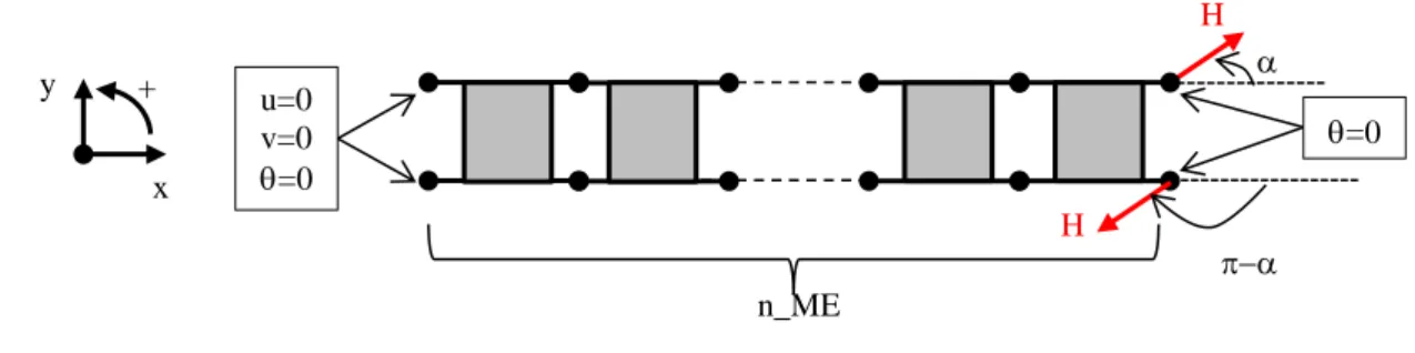
Mesh and boundary conditions. The bonded overlap is regularly meshed with a parametrical number n_ME of
18
bonded-beams elements. One extremity is clamped and the loading is applied under displacement (termed H) at
19
the other extremity where the bending angle is fixed (see Figure 6). The applied displacement is H=0.074 mm so
20
that the damage begins to propagate in the adhesive layer at the loaded extremity. In view of the application of
21
the inverse method, it is mandatory that the adhesive layer does not deform at the joint extremity where the load
22
is not applied. Clamping conditions avoid both peel and shear deformations.
15
1
Figure 6. Applied displacement H and fixed displacements for the MCB test configuration.
2
The results are not presented in this paper but a study on the influence of mesh size up to a maximal mesh
3
density of twenty ME per mm was performed under a pure linear elastic analysis under pure mode I (=/2).
4
The conclusions are that (i) the original approach and the present approach (see Appendix A) for the formulation
5
of the elementary stiffness matrix of ME provides exactly the same results, and (ii) the computed reaction as well
6
as the adhesive peak stresses do not vary at all with the mesh density.
7
Results. In order to assess the influence of the mesh density on the predictions from the ME model, four runs
8
associated with the four following mesh densities are launched: (i) one ME per mm, (ii) two MEs per mm, (iii)
9
four MEs per mm and (iv) eight MEs per mm. The norm of the reaction force on the loaded section of the upper
10
adherend as a function of the mesh density is provided in Figure 7. It is shown that the model converges when
11
the mesh density is increased. Moreover, the maximal peel and shear stresses at x=L reached during the runs are
12
constant when the mesh density varies and equal to: Smax=23.6 MPa and Tmax=19.8 MPa. This result is not
13
surprising since the load is applied under the shape of displacement at the location where the adhesive stress
14
evolution is observed and the stiffness matrix is updated considering the maximal value of both damage
15
parameters computed at each extremity of the ME.
16
H H u=0 v=0 =0 n_ME x y + =016
1
Figure 7. Norm of the reaction force on the loaded section of the upper adherend
2
3
2.3. Finite element model
4
Mesh and boundary conditions. A 3D FE model is developed using the FE code SAMCEF v18.1 (LMS PLM
5
software). This model makes use of linear brick elements with eight nodes and twenty-four degrees of freedom
6
for the adherends. A normal integration rule is selected. The adherends are assumed linear elastic. The adhesive
7
layer is simulated through 3D quadrangular interface elements. The CZM defined in section 2.1 is applied
8
through the Damage Interface SAMCEF material. The adhesive layer is regularly meshed along the overlap
9
length and width, with a constant aspect ratio equal to one: all the interface elements are squared. The adherends
10
mesh is coincident at the interface with the adhesive layer. The mesh along the thickness of adherends is
11
distributed as it follows. The adherends are cut at their own neutral plane in two parts. A distributed mesh is
12
applied on each part and a transition ratio equal to one is applied at the neutral plane. The size along the
13
thickness of the last element at the neutral axis of the adherend is fifty percent larger than those of the first
14
element at the interface with the adhesive layer. The same size ratio is applied for the second part. The mesh of
15
two adherend parts at the neutral plane is then coincident, so that a kinematic bonding of nodes is applied. As a
16
result, following the previous meshing method, the number of elements along the overlap drives the meshing of
17
the full model. The boundary conditions are relevant to those applied in the previous ME model. Only one half
18
of specimen is modelled and symmetry conditions are applied. The adherends are clamped at one extremity and
19
loaded under displacement at the other extremity (see Figure 8). It is indicated that the boundary conditions
20
6700 6750 6800 6850 6900 6950 7000 7050 7100 7150 7200 0 1 2 3 4 5 6 7 8 re ac tion for ce o n th e u p p e r ad h e re n d in N number of MEs17
applied on the FE element model are relevant to those applied on the ME model. In particular, at the loaded
1
extremity, the longitudinal displacement at the interface with the adhesive layer is the one at the neutral axis.
2
Nonlinear computation. The nonlinear computation is based on a Newton Raphson scheme, for which the
3
stiffness matrix is updated at each iteration with the secant properties concerning the adhesive layer. The
4
computation remains geometric linear, due the level of displacements and rotation. The applied displacement is
5
H=0.074 mm as for the simulations based on ME model. It is sufficient to apply the inverse method. As for the
6
simulations based on the ME model, each numerical test result is obtained from a simulation run involving one
7
hundred constant time steps t.
8
9
Figure 8. View of the 3D FE model on the symmetry plane including the mesh (two MEs per mm) and the
10
boundary conditions.
11
12
Results. As for the ME model, the influence of the mesh density on the predictions from the FE model is
13
assessed using the same 4 mesh densities. The maximal peel and shear stresses at x=L reached during the run is
14
provided in Figure 9 as a function of the mesh density. It is shown that these adhesive peak stresses converges
15
when the mesh density is increased, while tending to the adhesive peak stresses predicted by the ME model. For
16
a mesh density of eight element per mm, the relative difference in the FE model prediction from the ME model
17
prediction is -3.11% in peak peel stress and +0.90% in peak shear stress. The evolution of the adhesive peel
18
(shear) stress as a function of the opening (sliding) displacement at x=L for the FE and ME models with a mesh
19
density of eight elements per mm is provided in Figure 10 (Figure 11). A very good agreement is then shown
20
between the predictions of the FE and ME models.
21
22
u=0 v=0 u=H.cos() v=H.sin() u=-H.cos() v=-H.sin()18
1
Figure 9. Maximal peel and shear stresses at x=L reached during the run as a function of the mesh density for the
2
FE and ME models.3
4
5
6
7
8
19.5 20 20.5 21 21.5 22 22.5 23 23.5 24 0 1 2 3 4 5 6 7 8 ad h e si ve st re ss at x= L in M Panumber of elements per mm
[FE] peel stress [FE] shear stress
[ME] peel stress [ME] shear stress
0 5 10 15 20 25 0 0.005 0.01 0.015 0.02 0.025 0.03 p e e l st re ss S at x=L in M Pa opening displacement v in mm ME model FE model
19
Figure 10. Evolution of the adhesive peel stress as a function of the opening displacement at x=L for the FE and1
ME models with a mesh density of eight elements per mm.
2
3
4
Figure 11. Evolution of the adhesive shear stress as a function of the sliding displacement at x=L for the FE and
5
ME models with a mesh density of eight elements per mm.
6
7
2.4. Application of the inverse method
8
The inverse method is applied on the predictions of the ME model with a mesh density of eight element per mm.
9
Firstly, the J-integral parameter at x=L has to be computed according to Eq. (2). Taking benefit from the elevated
10
number of computation time, a simple numerical integration is then performed as:
11
𝐽(𝑡𝑓) = ∑𝑖=𝑓𝑖=1𝑇(𝑡𝑖)[𝛿𝑢(𝑡𝑖) − 𝛿𝑢(𝑡𝑖−1)] + ∑𝑖=𝑓𝑖=1𝑆(𝑡𝑖)[𝛿𝑣(𝑡𝑖) − 𝛿𝑣(𝑡𝑖−1)] (15)
12
where ti is the ith computation time, tf is the las computation time and t0 is equal to zero. It is indicated that this
13
computation of the J-integral is valid in the abscissa x=L only and at any time, because (i) the applied loading on
14
the neutral line in terms of u and v is the same as the one seen at the interface in x=L (=0) and (ii) the applied
15
loading is proportional at any time. As a result, the mixed mode parameter is constant at any time in x=L and
16
the shear (peel) stress is only dependent on u (v) at the given constant .
17
Secondly, the adhesive stresses are computed according to Eq. (5) and Eq. (6). The required differentiation of the
18
J-integral parameter is obtained by taken the slope between two consecutive times:
19
0 2 4 6 8 10 12 14 16 18 20 0 0.05 0.1 0.15 sh e ar str e ss T at x= L in M Pa sliding displacement u in mm ME model FE model20
{𝑆(𝛿𝑣(𝑡)) = 𝐽(𝑡)−𝐽(𝑡−𝛿𝑡) 𝛿𝑣(𝑡)−𝛿𝑣(𝑡−𝛿𝑡) 𝑇(𝛿𝑢(𝑡)) =𝛿𝐽(𝑡)−𝐽(𝑡−𝛿𝑡) 𝑢(𝑡)−𝛿𝑢(𝑡−𝛿𝑡) (16)1
The evolution of the adhesive peel (shear) stress as a function of the opening (sliding) displacement at x=L as
2
computed by the ME model with a mesh density of eight elements per mm and predicted by the inverse method
3
is provided in Figure 12 (Figure 13). It is shown that the predictions of the inverse method does not fit those of
4
the ME models. It is then concluded that the considered CZM is an example for which the inverse method fails
5
to predict the adhesive peel and shear stresses under mixed-mode. This example is not a general proof for this
6
type of CZM. However, the main fact is that the application of the inverse method associated with particular
7
types of CZM could lead to incorrect behavior assessment.
8
9
10
Figure 12. Evolution of the adhesive peel stress as a function of the opening displacement at x=L as computed by
11
the ME model with a mesh density of eight elements per mm and predicted by the inverse method.
12
13
0 20 40 60 80 100 120 140 0 0.005 0.01 0.015 0.02 0.025 0.03 p e e l st re ss S at x=L in M Pa opening displacement v in mm computed by ME model predicted by inverse method21
1
Figure 13. Evolution of the adhesive shear stress as a function of the sliding displacement at x=L as computed by
2
the ME model with a mesh density of eight elements per mm and predicted by the inverse method.
3
4
2.5. Description of the Direct Method
5
This method is presented in (Lélias 2016). It is based on the measurement around the crack tip of the
6
displacement of the neutral axis according to the x-axis and the y-axis. Contrary to the inverse method, no spatial
7
integration of equilibrium equations is required.
8
In the case of pure mode I loading, the adhesive shear stress vanishes so that the local equilibrium of adherends
9
can be reduced to the following set of differential equations for j=1,2:
10
{ 𝑑𝑁𝑗 𝑑𝑥 = 0 𝑑𝑉𝑗 𝑑𝑥 = (−1) 𝑗+1𝑏𝑆 𝑑𝑀𝑗 𝑑𝑥 + 𝑉𝑗= 0 (17)11
As a result, it comes:12
𝑆 = (−1)𝑗[−𝐵𝑗 𝑏 𝑑3𝑢𝑗 𝑑𝑥3 + 𝐷𝑗 𝑏 𝑑4𝑤𝑗 𝑑𝑥4] (18)13
Using the constitutive relationship, the adhesive peel stress can be expressed as:
14
𝑆 = (−1)𝑗 𝐷𝑗 𝑏 𝑑4𝑤𝑗 𝑑𝑥4 (19)15
In the case of pure mode II loading, the adhesive peel stress vanishes so that the local equilibrium of adherends
16
can be reduced to the following set of differential equations for j=1,2:
17
0 5 10 15 20 25 0 0.05 0.1 0.15 sh e ar str e ss T at x= L in M Pa sliding displacement u in mmcomputed with ME model predicted by inverse method
22
{ 𝑑𝑁𝑗 𝑑𝑥 = (−1) 𝑗𝑏𝑇 𝑑𝑉𝑗 𝑑𝑥 = 0 𝑑𝑀𝑗 𝑑𝑥 + 𝑉𝑗+ 𝑏ℎ𝑗𝑇 = 0 (20)1
As a result, it comes:2
𝑇 = (−1)𝑗[𝐴𝑗 𝑏 𝑑2𝑢𝑗 𝑑𝑥2 − 𝐵𝑗 𝑏 𝑑3𝑤𝑗 𝑑𝑥3] (21)3
Using the constitutive relationships, the adhesive shear stress can be expressed as:
4
𝑇 = (−1)𝑗 𝐴𝑗 𝑏 𝑑2𝑢𝑗 𝑑𝑥2 (22)5
In the case of mixed-mode I/II loading, the local equilibrium of adherends is given by Eq. (5). The following
6
expressions for the adhesive peel and shear stresses are obtained:
7
𝑆 = [(−1)𝑗 𝐷𝑗 𝑏 − ℎ𝑗 𝐵𝑗 𝑏] 𝑑4𝑤𝑗 𝑑𝑥4 + [ℎ𝑗 𝐴𝑗 𝑏 − (−1) 𝑗 𝐵𝑗 𝑏] 𝑑3𝑢𝑗 𝑑𝑥3 (23)8
𝑇 = (−1)𝑗[𝐴𝑗 𝑏 𝑑2𝑢𝑗 𝑑𝑥2 − 𝐵𝑗 𝑏 𝑑3𝑤𝑗 𝑑𝑥3] (24)9
The same hypotheses as for the ME model are used for the direct method, so that its application on numerical
10
test results with a suitable post processing method provides predictions exactly corresponding to those of ME. A
11
design of experiments is then developed to investigate the main factors influencing the predictions of the direct
12
method.
13
14
3. Assessing our methodology of derivatives of deflection with DIC experimental parameters
15
3.1. Signal processing of the 3rd order derivative of the deflection
16
Within the framework of the direct method, the evolution of the adhesive stresses can be theoretically derived
17
from the measurement at the crack tip of the second and third order derivative of the upper adherend bending
18
angle and of the derivative of the upper adherend longitudinal displacement at neutral axis (see section 2.5).
19
Since the raw differentiation of noised experimental results can lead to the rise of important numerical
20
singularities, a particular attention has to be given to the correct evaluation of these successive derivatives. Data
21
pre-processing is then highly needed to reduce experimental noises (see Figure 14). The data pre-processing
22
algorithm used to reduce experimental noises from the measured upper and lower adherends displacement fields
23
lies on the optimal sub-rank approximation (OSRA) based on singular value decomposition (SVD), and is
24
related to signal processing techniques that are commonly referred to as SVD signal enhancement methods,
25
reduced-rank signal processing or more simply subspace methods (Andrews and Patterson 1973). The detailed
23
presentation of the data pre-processing is not given in detail in this paper; a summarized description can be found
1
in the Appendix B.
2
3
Figure 14. Comparison of the 3rd order derivative of the deflection of the neutral fiber of the upper adherend
4
obtained from raw and pre-processed experimental results.
5
6
3.2. Supervised experiments using virtual fields
7
To characterize the ability of the suggested data pre-processing and differentiation algorithm to determine the
8
successive derivatives of the adherend-to-adherend displacement field with sufficient accuracy, we propose to
9
use supervised virtual fields. It refers to the data pre-processing and data differentiation of a displacement field
10
that is virtually generated so that the evolution of its successive derivatives is known in advance of the
11
experiment. For simplification purpose, the comparison between the supervised data and those obtained from the
12
data processing will be made in terms of the 3rd and 4th order derivatives of the transverse displacement of the
13
adherend neutral axis only. However the results are similar with other derivatives
14
The virtual displacement field is generated using Matlab® R2012b and resumes the kinematic of a classical
15
Euler-Bernoulli’s beam in coupled in-plane tension/flexion, so that:
16
{𝑢(𝑥, 𝑦, 𝑡) = 𝑢(𝑥, 𝑦 = 0, 𝑡) − 𝑦 𝜕𝑣(𝑥,𝑦=0,𝑡) 𝜕𝑥 𝑣(𝑥, 𝑦, 𝑡) = 𝑣(𝑥, 𝑦 = 0, 𝑡) (25)17
where the evolutions of u(x,y=0,t) and v(x,y=0,t) are arbitrary fixed as:
18
{𝑢(𝑥, 𝑦 = 0, 𝑡) = 𝑒−0.005𝑡𝑥
𝑣(𝑥, 𝑦 = 0, 𝑡) = 𝑒−0.15𝑡𝑥 (26)
19
To model the effect of experimental noises, the virtual displacement field described in Eq. (25) and Eq. (26) is
20
then degraded by adding a normal (Gaussian) noise using the normrand(0,σ) Matlab® function, where 0 refers to
21
the prescribed zero mean value and σ to the configurable standard deviation of the normal (Gaussian) noise
22
distribution.23
-2.0E-04 0.0E+00 2.0E-04 4.0E-04 6.0E-04 8.0E-04 1.0E-030.0E+00 2.0E-04 4.0E-04 6.0E-04 8.0E-04 1.0E-03
M eas ur ed d 3v/dx 3 Supervised d3v/dx3 Raw Supervised Pre-processed
24
In order to test for the linear dependency between the successive derivatives of the supervised data and those
1
obtained from the fitted polynomial series, the Pearson product-moment correlation coefficient is used:
2
𝑟 =√[𝑛 ∑ 𝑥𝑛(∑ 𝑥𝑦)−(∑ 𝑥)(∑ 𝑦)2−(∑ 𝑥)2][𝑛 ∑ 𝑦2−(∑ 𝑦)2] (27)
3
where x refers to the set of supervised data, y to the set of simulated data and n to the total number of data pairs.
4
5
3.3. Chosen DOE and justification
6
A full factorial Design of Experiments (DoE) consists in the following: (i) vary one factor at a time, (ii) perform
7
experiments for all levels and combination of levels for all factors, (iii) hence perform a large number of
8
experiments (N), (iv) so that all effects and interactions are captured. Let k be the number of factor, ni the number
9
of levels of the ith factor and p the number of replications to determine the impact of the measurement dispersion.
10
The total number of experiments N of a full factorial DoE is then:
11
𝑁 = 𝑝(∏𝑘𝑖=1𝑛𝑖) (28)
12
Here is considered a full factorial DoE of five factors with respectively 3x3x3x3x2 levels, so that the linear
13
Taguchi’s graph of effects and interactions can be represented in the form of Figure 15.
14
15
Figure 15. Linear Taguchi’s graph of main effects and interactions.
16
17
In Figure 15, the main effects and interactions are represented, termed respectively E(i) and I(ij), of factors i,j=A,
18
B, C, D and E onto the objective function that is r2.Each experiment is replicated 15 times to capture the impact
19
of the measurement dispersion, so that the total number of experiments is (3x3x3x3x2)x15=2430. The different
20
factor levels are given in Table 3.
21
22
23
24
: Effect of factor i (i=A,B,C,D,E) : First order interaction between i-j A B C D E Y = Y = M+E(A)+E(B)+E(C)+E(D)+E(E) +I(AB)+I(AC)+I(AD)+I(AE)+I(BC)+I(BD)+I(BE)+I(CD)+I(CE)+I(DE)
25
Table 3. Factor versus levels matrix.1
SNR-1 (A) x=y (B) t (C) Degree (D) Model (E) Low (-1) 0.00175 201 51 4 1
Medium (0) 0.00350 401 101 6 N.A High (+1) 0.00700 801 201 8 2
2
where SNR refers to the simulated Signal-to-Noise ratio, x=y to the spatial resolution of each displacement field
3
instantaneous image, t to the number of instantaneous images taken during the experiment (i.e. thereafter
4
referred as the temporal resolution), Degree to the degree of the polynomial series used to fit/differentiate the
5
neutral fiber transverse displacement and Model to the model used for minimizing the vertical deviation with
6
experimental data in the sense of the least squares method (1 means fitting independently on v(x) and on
7
θ(x)=dv(x)/dx, 2 means fitting simultaneously v(x) and θ(x)=dv(x)/dx).
8
9
3.4. Synthesis of the results
10
The initial SNR appears as a key parameter in increasing the accuracy of measuring the successive derivatives of
11
the upper adherend displacement field (see Figure 16-(a)), then suggesting that a significant attention has to be
12
given into reducing the noise of the measured signal before any pre-processing of the data. This can be achieved
13
in various ways so that it results in improving the overall quality of the displacement measures.
14
15
16
17
18
19
20
21
22
26
1
2
3
Figure 16. Effect of factor i (i=A,B,C,D,E) on the correlation coefficient r2. Influence of the experimental
4
(algorithmic) parameters on the accuracy of the experimental measures. Red= Significant effects. Black=
5
Negligible effects.
6
7
The spatial resolution of the instantaneous images of the upper adherend displacement field also appears as a key
8
parameter in increasing the accuracy of the estimation of the successive derivatives of the upper adherend
9
displacements (see Figure 16-(b), Figure 17-(e) and Figure 17-(h)). A particular attention has then to be given to
10
measuring the displacements of the upper adherend with a sufficient enough spatial resolution.
11
-0.15 -0.1 -0.05 0 0.05 0.1 0.15 -1 0 1 E( A ) Level of factor A E(A) -0.15 -0.1 -0.05 0 0.05 0.1 0.15 -1 0 1 E( B ) Level of factor B E(B) -0.15 -0.1 -0.05 0 0.05 0.1 0.15 -1 0 1 E( C ) Level of factor C E(C) -0.15 -0.1 -0.05 0 0.05 0.1 0.15 -1 0 1 E( D ) Level of factor D E(D) -0.15 -0.1 -0.05 0 0.05 0.1 0.15 -1 0 1 E( E) Level of factor E E(E) (a) (b) (c) (d) (e)27
1
2
3
4
5
-0.08 -0.06 -0.04 -0.02 0 0.02 0.04 0.06 0.08 -1 0 1 I(AB ) Level of factor B I(AB,A=-1) I(AB,A=0) I(AB,A=+1) -0.08 -0.06 -0.04 -0.02 0 0.02 0.04 0.06 0.08 -1 0 1 I(AC ) Level of factor C I(AC,A=-1) I(AC,A=0) I(AC,A=+1) -0.08 -0.06 -0.04 -0.02 0 0.02 0.04 0.06 0.08 -1 0 1 I(AD) Level of factor D I(AD,A=-1) I(AD,A=0) I(AD,A=+1) -0.08 -0.06 -0.04 -0.02 0 0.02 0.04 0.06 0.08 -1 0 1 I(B C ) Level of factor C I(BC,B=-1) I(BC,B=0) I(BC,B=+1) -0.08 -0.06 -0.04 -0.02 0 0.02 0.04 0.06 0.08 -1 0 1 I(B D ) Level of factor D I(BD,B=-1) I(BD,B=0) I(BD,B=+1) -0.08 -0.06 -0.04 -0.02 0 0.02 0.04 0.06 0.08 -1 0 1 I(CD) Level of factor D I(CD,C=-1) I(CD,C=0) I(CD,C=+1) -0.08 -0.06 -0.04 -0.02 0 0.02 0.04 0.06 0.08 -1 0 1 I(AE ) Level of factor A I(AE,E=-1) I(AE,E=+1) -0.08 -0.06 -0.04 -0.02 0 0.02 0.04 0.06 0.08 -1 0 1 I(B E) Level of factor B I(BE,E=-1) I(BE,E=+1) -0.08 -0.06 -0.04 -0.02 0 0.02 0.04 0.06 0.08 -1 0 1 I(CE ) Level of factor C I(CE,E=-1) I(CE,E=+1) -0.08 -0.06 -0.04 -0.02 0 0.02 0.04 0.06 0.08 -1 0 1 I(D E) Level of factor D I(DE,E=-1) I(DE,E=+1) (a) (b) (c) (d) (e) (f) (g) (h) (i) (j)28
Figure 17. First order interaction between factors i-j (i,j=A,B,C,D,E) on the correlation coefficient r2. Influence1
of the experimental (algorithmic) parameters on the accuracy of the experimental measures. Red= Significant
2
interactions. Black= Negligible interactions.
3
4
On another side, the time resolution (i.e. number of images of the upper adherend displacement field taken
5
during the experiment) appears as negligibly influencing the accuracy of the estimation of the successive
6
derivatives of the upper adherend displacements (see Figure 16-(c), Figure 17-(b), Figure 17-(d), Figure 17-(f)
7
and Figure 17-(i)). Thus its own effect as well as its respective interactions with other factors can be legitimately
8
neglected at first sight.
9
Similarly to the initial SNR or the spatial resolution of the displacement images, the degree of the polynomial
10
series used for fitting/differentiating the pre-processed displacements also appears as a parameter that has to be
11
chosen with extreme caution. Indeed, although increasing the degree of the polynomial series from 4 to 6 appears
12
as negligibly influencing the overall accuracy of the measure, increasing it from 6 to 8 results in a serious
13
degradation of the accuracy of the measure (see Figure 16-(d)). This degradation of the accuracy of the
14
measurement using high order polynomials is a well-known issue, and is due to the oscillation of the polynomial
15
series around the experimental set of data points for increasing degrees (i.e. Runge’s phenomenon). A particular
16
attention has then to be given in choosing the best compromise between fitting the experimental data points
17
using high order polynomials functions and preserving the overall accuracy of the measurement of its successive
18
derivatives.
19
Finally, the choice of the Moore-Penrose pseudo inverse model for minimizing in the sense of the least squares
20
method the vertical deviation between the polynomial function (i.e. used for fitting/differentiating the set of
21
experimental data points) and the experimental data points themselves appears as a worthwhile way of
22
influencing the accuracy of the measured displacement derivatives (see Figure 16-(e)). It is then suggested that
23
simultaneously accounting for both v(x) and θ(x)=dv(x)/dx when fitting/differentiating the experimental set of
24
data points significantly increases the accuracy of the measurement.
25
26
4. Experimental test campaign
27
The entire test campaign is performed on an electro-mechanical test machine (Ref: Instron AI735-1325).
28
4.1. Adherend bulk specimens
29
29
Each specimen is manufactured from a laminated aluminum-magnesium-silicon alloy (6060 series). A total of
1
three specimens are tested. The manufactured specimens are measured before the tests (see Figure 18). The
2
evolution of both the applied load and the resulting displacement are measured using the build-in machine load
3
and displacement cells. The loading speed is fixed at 0.5mm/min. The evolution of the specimen displacement
4
field is measured using the Digital Image Correlation (DIC) technique (see Figure 19). Both the evolution of the
5
axial deformation and the Poisson’s ratio of the samples are computed from the evolution of the specimen
6
displacement field. The specimens are displacement loaded using the build-in machine displacement command
7
instruction. The results obtained in terms of (a) the axial stress-strain evolution law and (b) the evolution of the
8
measured Poisson’s ratio as a function of the axial deformation in Figure 20. The aluminum alloy exhibits two
9
distinct phases. The first one, the linear elastic phase, appears as extremely limited compared to the whole
10
deforming capability of the material (i.e. ~3% of the whole deforming capability of the material). The second
11
phase, the plasticization phase, appears on another side as extremely important (i.e. ~97% of the whole
12
deforming capability of the material). To model the effective stress-strain evolution law of each adherend, it is
13
then decided to fit a trilinear elastic-plastic evolution law onto the results obtained (see Figure 21). The material
14
law identified is provided in Table 4. A Poisson’s ratio of 0.35 is considered.
15
16
17
Figure 18. Geometry of the aluminum bulk specimens.