Suivi des changements des utilisations/occupations du sol en milieu urbain par imagerie satellitale de résolution spatiale moyenne : le cas de la région métropolitaine de Montréal

(1)

Suivi des changements des utilisations/occupations du sol en milieu

urbain par imagerie satellitale de résolution spatiale moyenne:

Le cas de la région métropolitaine de Montréal

Par Feng Mei LANG

Département de Géographie Faculté des Arts et des Sciences

Mémoire présenté à la Faculté des études supérieures

en vue de l’obtention du grade de Maître ès sciences en géographie

Mai 2012

(2)

Monitoring Land Use/Land Cover Changes in Urban Areas Using Medium Spatial Resolution Satellite Imagery: the Case of the Montreal Metropolitan Area

(Suivi des changements des utilisations/occupations du sol en milieu urbain par imagerie satellitale de résolution spatiale moyenne: le cas de la région métropolitaine de Montréal)

présentée par : Feng Mei LANG

a été évalué par un jury composé des personnes suivantes :

Oliver SONNENTAG président-rapporteur François CAVAYA directeur de recherche Yves BAUDOUIN membre du jury

(3)

Abstract

Nowadays land use/land cover maps at regional scale are commonly generated with satellite data of medium spatial resolution (between 10 m and 30m). The National Land Cover Database (NLCD) in the United States and the Coordination of Information on the Environment (CORINE) Land Cover program in Europe, both based on LANDSAT images, are two typical examples. However, these maps become rapidly obsolete, especially in highly dynamic areas such as mega cities and metropolitan areas. In many applications, such as to monitor the water quality affected by the Land use/Land cover (LULC) change, the spread of invasive species, policy making for city managers, annual updating of LULC maps is required. Since 2007, the USGS offers access to ortho-rectified LANDSAT imagery free of charge. Both archived (since 1984) and recently acquired images are available. Without doubt, such data availability will stimulate the research on fast and cost effective methods and techniques for “continuous” regional land cover/use map updating using medium resolution satellite imagery.

The objective of this research was to evaluate the potential of such medium resolution satellite imagery for providing information on changes useful for the continuous updating of LULC maps at a regional scale in the case of the Montreal Metropolitan Community (MMC) area, a typical North American metropolis.

Previous studies have demonstrated that many factors could affect the results of automatic change detection such as: (1) the characteristics of the images (spatial resolution, spectral bands, etc.); (2) the method itself used to automatically detect changes; and (3) the complexity of the landscape. In the study site except for the Central Business District (CBD) and some commercial streets, land uses (industrial, commercial, residential, etc.) are well delimited. Thus this study was focused on the other factors affecting change detection results, namely, the characteristics of the images and the method of change detection. We used 6 spectral bands of LANDSAT TM/ETM+ with 30 m spatial resolution and 3 spectral bands of ASTER-VNIR with 15 m spatial resolution to evaluate the impact of image characteristics on change detection. Concerning the change detection method, we decided to compare two types of automatic techniques: (1) techniques providing information principally on the location of changed areas,

(4)

and (2) techniques providing information on both the location of changed areas and the type of changes ("from-to" classes).

The main conclusions of this research are as follows:

Change detection techniques such as image differencing or change vector analysis applied to LANDSAT multi-temporal imagery provide an accurate picture of changed areas in a fast and efficient manner. They can thus be integrated in a continuous monitoring system for a rapid evaluation of the volume of changes. The produced maps could be helpful to guide the acquisition of high spatial resolution imagery if a detailed identification of the type of changes is required.

Change detection techniques such as principal component analysis and post-classification comparison applied to LANDSAT multi-temporal imagery could provide a relatively accurate picture of “from-to” classes but at a very general thematic level (for example, built-up to green space and vice-versa, forest lands to bare soil and vice-versa, etc.). ASTER images with better spatial resolution but with less spectral bands than LANDSAT images do not provide more detailed thematic information (for example forest land to commercial or industrial areas).

The results indicate that future research should be focused on the detection of changes in the vegetation cover as medium resolution imagery is highly sensitive to this type of surface cover. Maps indicating the location and the type of changes in vegetation cover are in itself very useful for various applications, such as environmental monitoring or urban hydrology, and can be used as indicators on land use changes. Techniques such as change vector analysis or vegetation indices could be used to this end.

Keywords: Land Cover/Use, Urban areas, Change Detection, Medium Spatial-Resolution Satellite-Imagery, LANDSAT TM, LANDSAT ETM+, ASTER-VNIR.

(5)

Résumé

De nos jours les cartes d’utilisation/occupation du sol (USOS) à une échelle régionale sont habituellement générées à partir d’images satellitales de résolution modérée (entre 10 m et 30 m). Le National Land Cover Database aux États-Unis et le programme CORINE (Coordination of information on the environment) Land Cover en Europe, tous deux fondés sur les images LANDSAT, en sont des exemples représentatifs. Cependant ces cartes deviennent rapidement obsolètes, spécialement en environnement dynamique comme les megacités et les territoires métropolitains. Pour nombre d’applications, une mise à jour de ces cartes sur une base annuelle est requise. Depuis 2007, le USGS donne accès gratuitement à des images LANDSAT ortho-rectifiées. Des images archivées (depuis 1984) et des images acquises récemment sont disponibles. Sans aucun doute, une telle disponibilité d’images stimulera la recherche sur des méthodes et techniques rapides et efficaces pour un monitoring continue des changements des USOS à partir d’images à résolution moyenne.

Cette recherche visait à évaluer le potentiel de telles images satellitales de résolution moyenne pour obtenir de l’information sur les changements des USOS à une échelle régionale dans le cas de la Communauté Métropolitaine de Montréal (CMM), une métropole nord-américaine typique.

Les études précédentes ont démontré que les résultats de détection automatique des changements dépendent de plusieurs facteurs tels : 1) les caractéristiques des images (résolution spatiale, bandes spectrales, etc.); 2) la méthode même utilisée pour la détection automatique des changements; et 3) la complexité du milieu étudié. Dans le cas du milieu étudié, à l’exception du centre-ville et des artères commerciales, les utilisations du sol (industriel, commercial, résidentiel, etc.) sont bien délimitées. Ainsi cette étude s’est concentrée aux autres facteurs pouvant affecter les résultats, nommément, les caractéristiques des images et les méthodes de détection des changements. Nous avons utilisé des images TM/ETM+ de LANDSAT à 30 m de résolution spatiale et avec six bandes spectrales ainsi que des images VNIR-ASTER à 15 m de résolution spatiale et avec trois bandes spectrales afin d’évaluer l’impact des caractéristiques des images sur les résultats de détection des changements. En ce qui a trait à la méthode de détection des changements, nous avons décidé de comparer deux types de techniques automatiques : (1) techniques fournissant des informations principalement sur la localisation des changements et (2)

(6)

techniques fournissant des informations à la fois sur la localisation des changements et sur les types de changement (classes « de-à »).

Les principales conclusions de cette recherche sont les suivantes :

Les techniques de détection de changement telles les différences d’image ou l’analyse des vecteurs de changements appliqués aux images multi-temporelles LANDSAT fournissent une image exacte des lieux où un changement est survenu d’une façon rapide et efficace. Elles peuvent donc être intégrées dans un système de monitoring continu à des fins d’évaluation rapide du volume des changements. Les cartes des changements peuvent aussi servir de guide pour l’acquisition d’images de haute résolution spatiale si l’identification détaillée du type de changement est nécessaire.

Les techniques de détection de changement telles l’analyse en composantes principales et la comparaison post-classification appliquées aux images multi-temporelles LANDSAT fournissent une image relativement exacte de classes “de-à” mais à un niveau thématique très général (par exemple, bâti à espace vert et vice-versa, boisés à sol nu et vice-versa, etc.). Les images ASTER-VNIR avec une meilleure résolution spatiale mais avec moins de bandes spectrales que LANDSAT n’offrent pas un niveau thématique plus détaillé (par exemple, boisés à espace commercial ou industriel).

Les résultats indiquent que la recherche future sur la détection des changements en milieu urbain devrait se concentrer aux changements du couvert végétal puisque les images à résolution moyenne sont très sensibles aux changements de ce type de couvert. Les cartes indiquant la localisation et le type des changements du couvert végétal sont en soi très utiles pour des applications comme le monitoring environnemental ou l’hydrologie urbaine. Elles peuvent aussi servir comme des indicateurs des changements de l’utilisation du sol. De techniques telles l’analyse des vecteurs de changement ou les indices de végétation son employées à cette fin. Mots-clés : Occupations/utilisations du sol, milieux urbains, détection des changements, ETM+/TM LANDSAT, VNIR-ASTER.

(7)

List of Tables

Table 1: Building permits in Montreal region from 1995-2008 ... 4

Table 2: Land use and land cover classification system for use with remotely sensed images.... 10

Table 3: Spectral bands of LANDSAT 5/7 TM/ETM+ sensors in the solar spectrum... 16

Table 4: Spectral bands of ASTER VNIR sensor in the solar spectrum ... 16

Table 5: Summary of Change Detection Techniques as outlined in Singh (1989), Coppin and Bauer (1996), Lunetta and Elvidge (1998), Coppin et al. (2004) and Lu et al. (2003)... 19

Table 6: Image set used in this study... 25

Table 7: Solar exo-atmospheric spectral irradiance (ESUN; in W/(m2. μm) for LANDSAT 5 TM and LANDSAT 7 ETM+ ... 33

Table 8: The temperature and humidity of the time (hour) image acquired ... 34

Table 9: Unit conversion coefficient and solar exo-atmospheric spectral irradiances ... 40

Table 10: Areas of LULC cover change between 1994-2008 using the image-differencing method... 45

Table 11: Coefficients used in Tassled Cap transformation ... 46

Table 12: Change categories... 47

Table 13: Areas of LULC change in the period 1994-2008 ... 51

Table 14: Change Statistics using the NDVI images... 56

Table 15: Eigenstructure of the multi-temporal LANDSAT TM dataset (1994 and 2008)... 61

Table 16: Areas occupied by the classes identified using the PCA approach ... 66

Table 17: Cross tabulation table for 5 classes in 1994 and 2008... 70

Table 18: Change rate of each class in the year of 1994 to 2008 ... 70

Table 19: Error matrix from LULC map from PCA (between 1994-2008) ... 78

Table 20: Error matrix from LULC map of 1994 ... 79

Table 21: Error matrix from LULC map of 2008 ... 79

Table 22: Error matrix for LULC change map (PCC technique) ... 80

Table 23: LULC change between 2001-2007 from ASTER data (generated from figure 43) ... 93 Table 24: LULC change between 2001-2007 from LANDSAT data (generated from figure 44) 93

(10)

List of Figures

Figure 1: Angular IFOV and height above ground of the sensors define the size of the resolution cell... 11 Figure 2: Typical spectral signature for soil, green vegetation and dry vegetation. ... 12 Figure 3: Comparative results obtained with two types of medium spatial resolution images .... 14 Figure 4: One example for difference in spatial resolution between LANDSAT 30m data and ASTER 15m data in same spectral band: band 2... 15 Figure 5: Study sites: site I is the entire ubanized portion of the Montreal Metropolitan Community area ; site II is the area indcated by the yellowrectangle (see Figure 6) ... 26 Figure 6: Study site – II (False color composite of 1994 LANDSAT data : red-band4, green-band 3 and blue-band 2) ... 27 Figure 7: Procedures of the study ... 29 Figure 8: False color composition (R: band 4, G: band 3, B: band 2) of the LANDSAT TM 2008 image before the pre-processing ... 36 Figure 9: False color composition (R: band 4, G: band 3, B: band 2) of the LANDSAT TM 2008 image after the pre-processing (atmospheric effects removed) ... 36 Figure 10: ASTER image (2007) before de-stripping ... 38 Figure 11: ASTER image (figure 10) after destripping ... 38 Figure 12: ASTER 2007 data before pre-processing (false color composition: R: band 3, G: band 2, B: band 1)... 41 Figure 13: ASTER 2007 data after pre-processing (false color composition: R: band 3, G: band 2, B: band 1)... 41 Figure 14: LULC hange map between 1994 to 2008 using image differencing method... 44 Figure 15: Tasseled Cap Transformation of 1994 LANDSAT data (R: Brightness G: Greenness B: Wetness)... 48 Figure 16: Tasseled Cap Transformation of 2008 LANDSAT data (R: Brightness G: Greenness B: Wetness)... 49 Figure 17: LULC change map between 1994-2008 using the CVA method... 50 Figure 18: Spectral signatures of common surface materials in urban areas... 52 Figure 19: Comparison of the NDVI and NDBI calculated from LANDSAT images of 1994 and 2008... 53

(11)

Figure 20: Comparison of the NDVI and NDBI calculated from LANDSAT images of 1994 and

2008 after classification ... 55

Figure 21: LULC change map between 1994-2008 uisng NDVI method... 57

Figure 22: LULC change map between 1994-2008 uisng NDBI method ... 58

Figure 23: Comparison of the results obtained with the CVA and image differencing techniques ... 59

Figure 24: 12 components of composed image created by principal components analysis ... 62

Figure 25: PCA components color composition (R: first Eigenchannel G: second Eigenchannel B: third Eigenchannel) ... 63

Figure 26: Interactive training for a supervised classification of the first three principal components ... 64

Figure 27: LULC change map between 1994-2008 using the method of PCA ... 65

Figure 28: Classification map of LULC on 1994 (in 5 classes: built-up, forest, grass/golf course, water and barren land) ... 67

Figure 29: Classification map of LULC on 2008 (in 5 classes: built-up, forest, grass/golf course, water and barren land) ... 68

Figure 30: LULC change map between 1994-2008 uisng PCC ... 69

Figure 31: A: band 1 in grayscale B: 3 bands composition image (R band 1, G band 2 and B -band 3): the read pixels are the damged pixels ... 71

Figure 32: Error analysis for the classification map of 2008 and 1994 ... 72

Figure 33: LULC classification map of 1994 image with 7 classes ... 73

Figure 34: LULC classification map of 2008 image with 7 classes ... 74

Figure 35: A: 1994 ground truth data, derived from a mosaic of aerial photos acquired in dated April 1994 B: 2008 ground truth data, derived from combining QUICKBIRD images on Google Earth acquired in August 2008... 75

Figure 36: LULC change from forest to built-up... 76

Figure 37: LULC Classification Map on 2001 (with class wetland) ... 83

Figure 38: LULC Classification Map on 2001 (with class commercial/industrial)... 85

Figure 39: Classification of 2001 ASTER and 2001 LANDSAT images ... 87

(12)

Figure 41: Comparison of LULC Classification Map on 2001 and 2007 from LANDSAT data (using 3 bands and 6 bands)... 89 Figure 42: Comparison of LULC Classification Map on 2001 and 2007 from ASTER data and LANDSAT data (ASTER VNIR 3 bands and LANDSAT 3 bands) ... 90 Figure 43: LULC Change Map during 2001-2007 from ASTER data ... 91 Figure 44: LULC Change Map during 2001-2007 from LANDSAT data (6 bands) ... 92

(13)

List of abbreviations

ASTER Advanced Space-borne Thermal Emission and Reflection Radiometer CBD Central Business District

CLC CORINE Land Cover

CORINE Coordination of information on the environment CVA Change Vector Analysis

DN Digital Number

EROS Earth Resource Observation Science GIS Geographic Information System GLS2005 Global Land Surveys

GRS80 Geodetic Reference System ETM+ Enhanced Thematic Mapper Plus IFOV Instantaneous Field Of View LULC Land Use/Land Cover

MMC Montreal Metropolitan Community MSS Multiple Spectral Scanner

NAD83 North American Datum 1983

NASA National Aeronautics and Space Administration

NDBI Normalized Difference Built-up Index NDVI Normalized Difference Vegetation Index

NIR Near infrared reflectance NLCD National Land Cover Dataset PCA Principle Component Analysis

(14)

PCC Post Classification Comparison SWIR Short Wave Infrared

TM Thematic Mapper

USGS United States Geological Surveys. Geological Survey

UTM Universal Transverse Mercator VNIR Visible Near-Infrared

(15)

Dedications

To my father, who taught me to never give up and this will stay in me forever. To my family members, who helped and encouraged me to complete this thesis.

I want to offer you my gratitude for all your support and I love you all. Without your support, this thesis would be impossible to materialize.

(16)

Acknowledgements

I want to thank my supervisor, Dr. Francois Cavayas, for his endless support in every step of this study. His advice and encouragement made it possible for me go through all the difficulties during the study. Specially, his sense of humor cheered me up when I was really down periodically.

Also, I would like to take this opportunity to offer my gratitude to my colleges, Dr. Robert Cissoko and Dr. Robert Fiset, for their support. Moreover, I would also like to express my gratitude to my employer Mr. Dick Johnsson for providing me a flexible work schedule enabling me to do my study.

This thesis would not be complete without data, which was provided by the LP DAAC (Land Processes Distributed Active Archive Centre) and USGS (United States Geological Survey) for the ASTER and LANDSAT satellite imagery data.

(17)

Chapter 1 Introduction

1.1 Land Use/Land Cover Change Monitoring in Urban Territories:

Problem Statement

Land Use/Land Cover (LULC) inventories and maps in urban territories provide basic information to various application fields including: territorial management and planning, traffic studies, modeling and planning of public transportation, studies in environmental quality, urban climatology and urban hydrology. According to Jensen (2005), land use refers to what people do on the land surface, such as agriculture, commercial, residential, and transportation whereas land cover is the type of material present in the landscape such as water, vegetation, soil, and man-made materials. Taxonomy systems used for mapping purposes are hierarchical in nature with the most generalized level, a blend of land cover and land use categories such as built-up and urban areas, agriculture, forests, and rangeland. Such thematic levels are depicted on small scale maps (e.g. 1:250 000 or smaller) and are often used for studies at the national level. At more detailed levels, land use categories are almost exclusively defined. In built-up and urban areas categories such as single- or multi-family residential areas, chemical industries, and shopping centers are specified. These categories are depicted on medium and high scale maps helpful for studies at regional and local levels (Anderson et al. 1976). Thus, in general, taxonomy systems and corresponding maps are usually termed as LULC taxonomy systems and maps.

Change detection is defined as the process of identifying differences in the state of an object or phenomenon by observing it at different times (Singh, 1989). In the context of LULC mapping, change detection is applied principally for the updating of LULC maps. In fact, these maps can become rapidly obsolete especially in urban territories due to the densification of the built-up area and the urban sprawl.

Remotely sensed images, either space-borne or airborne, play an important role in mapping land use patterns and updating LULC maps. Ortho-photography and digital aerial or satellite imagery of high spatial resolution are used for mapping LULC at large scales, mostly by visual interpretation, while space-borne imagery of medium (10m~50m) spatial resolution is

(18)

used for mapping LULC at regional and national scales, mostly by digital analysis and classification.

Based on medium (10-50m) resolution imagery provided by various satellite missions (LANDSAT, SPOT, IRS, etc.), programs of systematic LULC mapping at regional scales and map updating come into being worldwide. In the United States, for example, two generations of the National Land Cover Dataset (NLCD), a component of the USGS Land Cover Characterization Program, has been released covering the United States. The first generation, NLCD 1992, was produced for the conterminous United States on the basis of 1992 LANDSAT Thematic Mapper (TM) imagery and supplemental data by the U.S. Geological Survey (USGS), in cooperation with the U.S. Environmental Protection Agency. The second generation, NLCD 2001, was released on 2007. It is produced on the basis of LANDSAT Enhanced Thematic Mapper (ETM+) imagery covering the entire U. S. A., including Hawaii, Alaska, and Puerto Rico. A third generation, NLCD 2006, is underway based on LANDSAT images of 2006. The method used to generate the NLCD 2006 dataset is to detect changed areas between 2001 and 2006, classify them and integrate the results into the NLCD 2001 dataset. The NLCD datasets are distributed in 30m resolution.

CORINE (Coordination of Information on the Environment) Land Cover (CLC) Data is another important application of LANDSAT satellite imagery. Two generations have been released in resolution of 100m. The first generation, CLC 1990, has been produced in 1996 for most of the European countries based on the 1990 LANDSAT TM. The second generation, CLC 2000, has been produced in 2007 based on 2000 LANDSAT 7 ETM+. The method to generate CLC 2000 is to detect the changes between the images acquired in 2000 and in 1990, similar to the method used by the USGS for NLCD 2006. The detected changes are then classified and integrated to the dataset CLC 1990 to create the dataset CLC 2000.

In Canada, LULC maps for the entire country are not available at scales similar to the above mentioned map series. Two governmental programs of the Ministry of Environment intended to systematically mapping LULC in rural and urbanized areas with provision to actualize them in regular intervals, the Canada Land Inventory and the Canada Land Use Monitoring Program (CLUMP), are abandoned since many years. Only some land cover datasets

(19)

are presently available to the public, such as the Circa-2000 Northern Land Cover of Canada at 30 m resolution, covering the North Provinces derived from LANDSAT 5 TM and LANDSAT-7 ETM+ between the years of 1999-2001 (Olthof et al., 2009), and the Ontario Land Cover data derived from LANDSAT TM imagery from the early 1990s. Local governmental agencies in urban communities and municipalities maintain LULC mapping activities and update their maps more or less at regular intervals, usually every 5 years or even more. However, such an updating rate, although responding relatively well to the needs of territorial managers and planners, is not adequate to support studies related to other application fields such as transportation modeling, environmental quality monitoring, etc. For these applications, especially in highly dynamic areas such as Metropolitan communities and mega-cities, a continuous monitoring of changes is the optimum. To illustrate this we present as an example the situation in the Montreal Metropolitan Community (MMC) area, our study site. The MMC, like other metropolitan areas of the world, shows rapid changes in land use/land cover, especially from the late nineties. The value of building permits is a good indicator of the rapidity of changes. According to Statistics Canada, this value from less than 2 billion dollars in 1995 peaks over 6.5 billion dollars in 2007. Even though there is a slight decrease in 2008, the value is still up to 6.4 billion CAD. Detailed information is listed in Table 1. Many new constructions have been developed in vacant lands and even some industrial or recreation lands, converted to residential areas. According to a recent study by Cavayas and Baudouin (2008) within the urban perimeter of the MMC area, vacant lands are built-up in at a rate of about 7 km2 _{per year. This development has an important effect}

especially in the forest land cover. Only in the Montreal Island in the period between 1999 and 2005, 18% of the forest lands (private sector) were lost converted mostly to residences (Cavayas and Baudouin, 2008). This phenomenon has therefore been causing increased land consumption and the continuous modification in the status of land use/land cover over time. An evaluation of the nature of these changes at an annual rate is thus important for the pre-mentioned applications. Since 2007, USGS offers free of charge access to ortho-rectified LANDSAT imagery (from 1984 to present) as well as to other imagery types of medium spatial resolution (ASTER imagery data covering U.S.A.). Every year at least one cloud-free LANDSAT image could be found covering any part of the world. It is thus interesting to examine if this type of imagery

(20)

could constitute the basis for a continuous monitoring of changes in LULC in metropolitan areas such as the Montreal one.

Table 1: Building permits in Montreal region from 1995-2008

Year Total residential and non-residential (dollars -thousands) Total residential (dollars -thousands) Residential percent of the total building permits Total built permits dollar _Percent Change (year-to-year) Residential permits dollar_ Percent Change (year-to-year) 1995 1,933,651 860,466 44% ---- ----1996 1,954,863 965,938 49% 1.1 12.3 1997 2,414,381 1,216,638 50% 23.5 26 1998 2,781,922 1,310,796 47% 15.2 7.7 1999 2,935,141 1,536,451 52% 5.5 17.2 2000 3,239,861 1,637,948 51% 10.4 6.6 2001 4,218,111 1,892,141 45% 30.2 15.5 2002 4,604,357 2,731,273 59% 9.2 44.3 2003 5,278,343 3,453,246 65% 14.6 26.4 2004 6,232,700 4,356,745 70% 18.1 26.2 2005 5,800,395 4,094,856 71% -6.9 -6 2006 6,034,021 3,955,144 66% 4 -3.4 2007 6,506,449 4,062,093 62% 7.8 2.7 2008 6,442,007 4,252,441 66% -1 4.7

(Source: Statistics Canada 2009. CANSIM table 026-0006. Retrieved from

http://www.statcan.gc.ca/datawarehouse/paiement/paiement.cgi?demande_id=200910151550085 5613 (October 15 2009))

1.2 Study objectives and hypotheses

Automatic change detection methods, usually applied with medium resolution imagery, imply the comparison of geometrically compatible multi-temporal images on a pixel by pixel basis. These methods could be divided into two broad categories (Lu et al., 2003): (i) methods indicating only the location of changed areas and (ii) methods providing both the location and the type of changes (“from-to” classes). Methods of the first category are based on spectral signatures comparison and could be used to provide information on material cover changes such as vegetation lost (or gained). Such information is valuable for studies related especially to

(21)

environmental quality evaluation (Cavayas and Baudouin, 2008). On the other hand, these maps could be used as a basis for obtaining higher resolution imagery covering areas that have major changes. Methods of the secondary category are based on different classification algorithms and could provide information useful for studies seeking to understand the trends in the development of urban areas for modeling or territorial planning purposes. As demonstrated by many previous studies with medium resolution imagery of the LANDSAT type (30 m spatial resolution) in urban areas only general classes of LULC could be extracted with sufficient accuracy such as built-up, forest lands, grasslands and water (e.g., Cavayas and Baudouin, 2008). Under some particular circumstances, depending mostly on the structure of the urban territory, more detailed categories can be extracted such as residential and commercial/industrial, especially in the outskirts and in the urban fringe. Such detailed categories are more easily extracted with imagery of relatively finer resolution (10-20 m).

Few attempts have been made to evaluate the potential of both approaches for the multi-temporal analysis of medium resolution multispectral images for LULC change monitoring in the Montreal region. The most recent study was done by Cavayas and Baudouin (2008) in the context of the “Biotope” project. This project was aiming at the examination of the correlation between LULC and changes in the thermal environment in the Montreal Metropolitan Community Area for the period 1984-2005. However, the approach employed for change detection was the so-called “map guided” change detection. In this approach the existing LULC map is compared to a recently acquired image and as that this method is more oriented to LULC map updating rather than change monitoring.

For all these reasons we decided to confine the following objectives of our study:

(a) Examine the possibilities of LANDSAT multispectral images to provide accurate information on the location of changed areas using comparison methods based solely on spectral signatures. Given the number of available spectral bands and their location in the solar spectrum spanning blue, green, red, near infrared, and short wave infrared wavelength ranges. We hypothesize that these images could effectively provide such information being sensitive especially to vegetation cover changes.

(22)

(b) Study the possibilities of LANDSAT multispectral images to provide accurate information on the type of changes specifically applied to the Montreal Metropolitan Community area. Regarding the level of detail on LULC extractible from these images in the Montreal area, only limited evidence exists in the literature provided by a study of Desjardins and Cavayas (1991). The authors using a LANDSAT TM image and visual interpretation criteria found that it was possible to identify within the built-up area without particular difficulties only the residential and some industrial areas. Categories characterized by vegetation cover such as parks, golf courses and forested areas, were easily identified. Thus we hypothesize that using classification algorithms based on spectral signature of objects, only general LULC categories should be extractible from LANDSAT images with sufficient accuracy even in the case of the Montreal urban environment.

(c) Compare the performance of other types of images of better spatial resolution available from the USGS to that of LANDSAT images concerning the identification of the type of changes. Among the available images, only these 15 m resolution VNIR images which provided by the ASTER sensor onboard of the experimental TERRA satellite present a particular interest in the context of change monitoring. However, the spatial coverage of one VNIR image is only about 10% of LANDSAT coverage and much less relatively frequent covering of the Montreal area (from 2000 to present). To the best of our knowledge, no studies of the Montreal area using this type of imagery exist. We hypothesize that the change in resolution from 30 m to 15 m should have an impact on the minimum size of detected areas of change. This is important in the case of existing sparsely built-up areas. It is less important in the case of newly developed areas mainly in the outskirts of urban areas. Concerning the level of detail, we expect that the identification of some categories within the built-up area should be easier than with LANDSAT images.

(23)

1.3 Structure of the thesis

This thesis is organized into seven chapters. The first chapter provides background and rationale for the study and research objectives. The second and third chapters are literature reviews and outline the results of previous studies on LULC mapping using medium spatial resolution imagery and on the automatic change detection techniques, respectively. Chapter four describes the framework of this study, including the study site, the images used in this study and the pre-processing as well as the methodological approaches. Chapter five explains how the data have been processed for detecting the LULC changes in the case of LANDSAT images. Chapter six compares the results of change detection obtained with ASTER-VNIR and LANDSAT imageries. Finally, chapter seven presents the main conclusions of this study.

(24)

Chapter 2 Mapping LULC from Medium Resolution

Multi-spectral Imagery

2.1 Introduction

The aim of our study is to examine the potential of medium resolution imagery for LULC change to monitor in urban areas. Thus first of all we have to define the topology of LULC extractible from this imagery. The next section is a brief review of the classification schemes used in LULC mapping. As also mentioned we would like to study the possibilities of various types of medium resolution imagery readily available free from the USGS services. More specifically we are interested in LANDSAT imagery (TM or ETM+) and to ASTER -VNIR imagery. The former is a multispectral imagery with six bands covering almost the entire solar spectrum (visible, near- and shortwave-infrared) with 30 m spatial resolution while the latter is a multispectral imagery with three spectral bands (green, red and near-infrared) of finer resolution (15 m) than the LANDSAT images. So the question addressed in this study is how the interpretation of spatial and spectral resolution affects the change-detection results. Section 2.3 presents a review of studies addressing this particular question.

2.2 LULC Classification Schemes

The best way to ensure that useful information on urban LULC is derived from remotely-sensed data is to base our work on a standardized LULC scheme (Chen and Stow, 2003). Many LULC classification schemas have been developed, such as: (a) the Land-Base Classification Standard (LBCS) developed by the American Planning Association (2006); (b) the CORINE (Coordination of information on the environment) in Europe; (c) the PELCOM (Pan-European Land Cover Monitoring) and (d) the USGS LULC classification system for use of remotely-sensed data. In North America and in the context of remote sensing image analysis, the standard LULC classification system is the USGS (Anderson et al., 1976), even though each city or urban community may have a slightly different system. This last scheme (d) was adopted since our study area was the Montreal Metropolitan territory.

(25)

USGS LULC classification system is a four level hierarchical taxonomy system. Table 2 shows the first two levels accessible, in principle, from medium resolution imagery (Jensen 2007): Level I (9 classes) and Level II (37 classes).

(26)

Table 2: Land use and land cover classification system for use with remotely sensed images

(Adopted from Jensen, 2007)

Level I Level II

1 Urban or Built-up Land

11 Residential

12 Commercial and Services 13 Industrial

14 Transportation, Communications, and Utilities 15 Industrial and Commercial Complexes 16 Mixed Urban or Built-up Land 17 Other Urban or Built-up Land

2 Agricultural Land

21 Cropland and Pasture

22 Orchards, Groves, Vineyards, Nurseries, and Ornamental Horticultural Areas 23 Confined Feeding Operations

24 Other Agricultural Land 3 Rangeland (Grass)

31 Herbaceous Rangeland 32 Shrub and Brush Rangeland 33 Mixed Rangeland 4 Forest Land

41 Deciduous Forest Land 42 Evergreen Forest Land 43 Mixed Forest Land

5 Water

51 Streams and Canals 52 Lakes

53 Reservoirs 54 Bays and Estuaries 6 Wetland 61 Forested Wetland

62 Non-forested Wetland

7 Barren Land

71 Dry Salt Flats 72 Beaches

73 Sandy Areas other than Beaches 74 Bare Exposed Rock

75 Strip Mines Quarries, and Gravel Pits 76 Transitional Areas

77 Mixed Barren Land

8 Tundra

81 Shrub and Brush Tundra 82 Herbaceous Tundra 83 Bare Ground Tundra 84 Wet Tundra 85 Mixed Tundra 9 Perennial Snow or Ice 91 Perennial Snowfields

(27)

2.3 Spatial Resolution vs. Spectral Resolution

2.3.1 Definitions

Spatial resolution refers to the size of the smallest feature depicted on a map or visible on an image. Two major factors are affecting the spatial resolution of the images: the size of the resolution cell and the contrast between the object and the surrounding ground. The resolution cell is defined by the instantaneous-field-of-view (IFOV) and the height of the sensor (Figure 1). In practice, when speaking about spatial resolution we refer to the size of the resolution cell by ignoring the impact of the contrast. In fact, as one sole radiance measurement of the sensor corresponds to the entire resolution cell, the size of the object has to be at least equivalent to the size of the resolution cell to de distinguishable on the image. However this is not always the case, since an object of the size of a resolution cell could be “undetectable” if it presents a low contrast with its surrounding ground. On the contrary, some high contrast features such as narrow rivers and canals or roads are visible even if their width is less than the sensor’s resolution cell. Many practitioners use as a rule of thumb that an object to be not only detected but also identified has to have a size at least 4 times the resolution cell of the sensor (Colwell, 1983).

Figure 1: Angular IFOV and height above ground of the sensors define the size of the resolution cell.

(28)

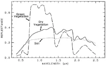
Spectral resolution, on the other hand, is the number and width of specific wavelength interval (bands/channels) in the electromagnetic spectrum to which a remote sensing instrument is sensitive. Bands/channels refer to recorded radiances by the sensor in different portions of the electromagnetic spectrum for the same material on the ground. As indicated by Colwell (1983), the surface of the Earth is illuminated by the sun’s radiation covering a large spectrum of wavelengths. Different materials have different characteristic absorption when solar radiation impinges on them. For instance, vegetation has a relatively strong absorption around the red wavelength. What is not absorbed by an object is reflected into space and is partially captured by the sensor. The reflection capacity of a material through the solar spectrum is described by its spectral signature (Figure 2). These signatures are often used in remote sensing as a means to identify LULC classes. Thus a multispectral sensor with fine spectral resolution offers a higher discrimination potential of ground features than another with few spectral bands (Colwell (1983).

Figure 2: Typical spectral signature for soil, green vegetation and dry vegetation. (Adopted from Rencz, 1999)

2.3.2 Previous findings

Very few studies addressed the question of how both spectral and spatial resolutions affect the discrimination capacity of LULC on medium-resolution satellite images especially in urban environments. Concerning the spatial resolution we have to go back in the 1980’s and the study of Welch (1985). The author compared two types of satellite images over an urban

(29)

environment of Athens in Greece, LANDSAT TM (30 m) and merged panchromatic and multispectral SPOT HRV imagery (10 and 20 m respectively), simulated from airborne images. Enhanced false color composites created from these images were then visually interpreted. Figure 3 reproduces the principal results of this study. Figure 3-b shows that the taxonomy system used in their study included Level II and III categories of the USGS system. The impact of change in image resolution from 30 m to 10 m is obvious comparing the obtained LULC maps (figure 3-a). The accuracies per LULC category was about 80% and even better with simulated SPOT images. Whereas in the case of simulated TM images the accuracy is about 60% (figure3-c). The authors note also that the application of automatic classification techniques was not successful to give thematic detail at the Level II and III categories.

Figure 4 shows an example of the impact on the visual appearance of an urban environment by choosing the resolution of the imageries from 30m to 15m used in this study (chapter 4). According to the results of Welch (1985) and given the fact that our study is based entirely on digital image analysis, it is expected that the application of ASTER will provide higher accuracy in classifying our images at least at the Level II of the USGS. A study for Phoenix metropolitan area by Waler and Blaschke (2008) using the method of object-oriented LULC classification to analyze the image in 0.61 m resolution acquired by a sensor called Landiscor with 3 bands (RGB). The overall accuracy is about 80% in Level II categories with 5 classes: soil, grass, woody, building and impervious. The major confusion for this study is caused by the big shadows of objects and to find the ‘best’ segmentation for a classification of many land-cover types with different sizes, shapes, and spectral characteristics. Based on this study, it shows that only the improvement of the resolution of spatial resolution will not able to derive more accurate classification result. The object-oriented classification technique is different with the techniques based on spectral per pixel (more in chapter 3). It is first introduced in the 1970s (de Kok et al. 1999). However, the method was limited by hardware, software, poor resolution of images and interpretation theories (Flanders et al. 2003). With an increase in hardware capability and availability of high spatial resolution images, specially, after the first commercial IKONOS 4 m MMS images available, the demand for object-oriented analysis has also increased (de Kok et al. 1999) because the techniques of "per-pixel" are no longer adequate for high resolution (less than 10 m) images. Due to the high cost of purchasing the high

(30)

resolution imageries, this study are only focus on these medium resolution images with free access from USGS.

a

b c

Figure 3: Comparative results obtained with two types of medium spatial resolution images (Adopted from Welch, 1985)

(31)

Figure 4: One example for difference in spatial resolution between LANDSAT 30m data and ASTER 15m data in same spectral band: band 2

A study by Herold et al. (2003) indicates, however, that these expectations have to be lowered since ASTER-VNIR images are poorer in terms of spectral resolution (Table 4) compared to LANDSAT images (Table 3). Even if this study concerns the classification of surface materials (asphalt, metal roof, water, vegetation, etc.), it provides interesting cues to understand the impact of spectral resolution alone. The authors using standard spectral signatures first established 14 narrow spectral bands in the solar spectrum useful for recognizing 25 different materials common in urban environments. A hyperspectral airborne image (224 spectral bands) was then used as a basis to simulate the signal which would be measured with the far more large spectral bands of two multispectral sensors while maintaining the spatial resolution fixed. The first simulated sensor is the IKONOS having four spectral bands (blue, green, red and NIR) while the second was the LANDSAT TM with six spectral bands (Table 3) in the solar spectrum. The hyper-spectral image and the two multispectral simulated images were then classified and the classification results quantitatively assessed. As expected, the best classification results of the 25 materials were obtained with the hyperspectral imageries. The accuracy is about 70%. Classification using the simulated IKONOS images produced a score 30% lower than those using the hyper spectral imageries, while the classification of the simulated TM image was only 13% lower. This higher performance of the TM image is explained by the presence of the two bands in the SWIR not available in the case of the IKONOS image. However, as the authors stress many misinterpretations exist between materials having

(32)

similar spectral signatures, such as the soil of bare land the concrete of built-up. Thus even if the hyperspectral imagery includes the 14 optimal bands global classification accuracy is lower than 70%.

In conclusion, the impact of both spatial and spectral resolution in the quality of LULC mapping and change detection is largely unexplored and in this sense, our study will contribute to find an answer to the question addressed in this section.

Table 3: Spectral bands of LANDSAT 5/7 TM/ETM+ sensors in the solar spectrum LANDSAT TM/ETM+ Spectral Sensitivity (µm) Nominal Spectral Location Band 1 0.45-052 Blue Band 2 0.52-0.6 Green Band 3 0.63-0.69 Red Band 4 0.76-0.9 Near-IR Band 5 1.55-1.75 Shortwave-IR Band 7 2.08-2.35 Shortwave-IR

(Source: adopted from USGS, retrieved from

http://LANDSAT.usgs.gov/about_mission_history.php)

Table 4: Spectral bands of ASTER VNIR sensor in the solar spectrum ASTER_VNIR Spectral Sensitivity_(µm) Nominal Spectral_Location

Band 1 0.52-0.60 Green

Band 2 0.63-0.69 Red

Band 3N 0.78-0.86 Near-IR

(Source: adopted from USGS, retrieved from

(33)

Chapter 3 Methods for LULC change detection based on

medium resolution multitemporal imagery

3.1 Basic Concepts

According to Green et al. (1994) change detection implies the comparison of the spatial representation of the same area in two different times and the measure of differences in the variables of interest while controlling differences caused by variables that are not of interest. In the case of comparison of multi-temporal remotely-sensed images the variable of interest is usually the spectral signature of objects included in the same area. A significant difference in spectral signatures means a change in the land cover. However as measured radiances are influenced by many other factors such as solar illumination conditions and atmospheric conditions during image acquisition, the direct comparison of images could lead to erroneous results. In order to obtain optimal results specific spatial, temporal, spectral and radiometric data issues have to be addressed. A typical list of criteria would include the following issues (Coppin

et al., 2004; Jensen et al., 1997; Lunetta and Elvidge, 1998; Millward et al., 2006):

 The sensors should have similar sensitivity imaging - ideally, the data from the same sensor has to be used to minimize spectral, radiometric and spatial resolution differences;

 The images should be from the same time of year or season to minimize solar illumination angle effects and differences in seasonal vegetation cover;

 The images should be co-registered to better than one half pixel accuracy to minimize spatial offset and distortion,

 Radiometric normalization may be necessary in order to remove atmospheric effects – differences caused by scattering and absorption by atmospheric constituents, and by differing solar zenith angles.

In the past four decades, there have been many studies proposing various algorithms for obtaining LULC change information using a wide variety of remotely sensed data. Lu et al. (2003) provides an extensive review of these studies. According to these authors the proposed algorithms for change detection can be categorized into two main categories. The first category

(34)

includes methods focused on the detection of detailed change trajectories (“from-to” classes), and the second focuses on detection of binary change and non-change features. Post-classification comparison is the most often used approach to detect detailed "from-to" change trajectory; while image differencing, image rationing, vegetation index differencing, and principal component analysis (PCA) are often used to detect binary change and non-change information. The adopted methods in this study in both categories are presented in the next section.

3.2 Adopted Automated Change Detection Techniques

Few studies present comparative results of the various change detection approaches. The most relevant ones are briefly summarized here. Civco et al. (2002) used five LULC change detection methods - post–classification cross tabulation, cross correlation analysis, neural networks, knowledge–based expert systems, and object–oriented classification. Nine land use/cover classes were selected for analysis. It was observed that there were merits to each of the five examined methods, and no single approach can solve the land use change detection problem. Mas (1997) tested 6 change detection techniques using LANDSAT Multi-Spectral Scanner (MSS) images for detecting areas of changes in the region of the Terminos Lagoon, Mexico. The change detection techniques considered were image differencing, vegetation index differencing, principal components analysis (PCA), direct multi-date unsupervised classification, post-classification change differencing and combination of image enhancement and post-post-classification comparison. The accuracy of the results was evaluated by comparison with aerial photographs through Kappa coefficient calculation. Besides providing information on the nature of changes, post-classification comparison was found to be the most accurate procedure. The author also pointed out that methods based on classification were found to be less sensitive to spectral variations and more robust when dealing with data captured at different times of the year. Yuan

et al. (2005) found also that the post classification comparison method provides good-accuracy

results (between 80% and 90%) when applied to LANDSAT images of the Twin Cities (Minnesota) Metropolitan Area. In his particular study the emphasis was put on the generation of transition matrix (“from-to” classes).

Based on the merits and complexity of the studies cited earlier, we decided to compare four automated change detection techniques in the case of our study area: (1) image differencing,

(35)

(2) change vector analysis, (3) principal components analysis, and (4) post-classification comparison. Table 5 summarizes the advantage and disadvantages of these four methods.

Table 5: Summary of Change Detection Techniques as outlined in Singh (1989), Coppin and Bauer (1996), Lunetta and Elvidge (1998), Coppin et al. (2004), and Lu et al. (2003)

Technique Method Advantage Disadvantage

Image differencing

Subtraction of multi temporal imagery on a spectral band

basis-original or transformed data

Simple and easy to interpret

Cannot provide transition matrix ("from-to" classes) and requires the definition of a threshold

Change Vector analysis

Multivariate change detection that exploits

the full

dimensionality of the image data; Produce two outputs: change

magnitude and change direction Ability to process any number of spectral bands desired and to provide detailed change information

Difficult to identify land cover change trajectories

Principal component analysis (PCA) Applied to two-date imagery to produce uncorrelated data; variations in land-covers are usually appear in specific principal components

Reduces data redundancy between bands and

emphasizes different information in the derived components

Requires comprehensive knowledge of the study

area; the changes are often difficult to interpret

and to label because of PCA depending on the input data statistics; it

cannot provide a complete matrix of change classes and need

to determine the thresholds to identify the

changed areas

Post classification

comparison

Spectral classification of each image in the

multi-temporal set; comparison of the classified images on pixel-by-pixel basis Minimizes impacts of differences caused by atmosphere, sensor and environment between multi-temporal images; provides a complete matrix of change information Requires comprehensive knowledge of the study

area; time consuming; final accuracy depends

on the result of classification of each

date

(36)

3.2.1 Image Differencing

Image differencing is a commonly used technique to rapidly locate changed areas by subtracting pixel values in a specific spectral band of two or more images of the same area acquired at different times (Coppin and Bauer 1996; Lunetta and Elvidge 1998, Coppin et al. 2004). To use this technique effectively, it requires a process of rigorous normalization of the data to the same geometric and radiometric referential. In the case of rugged terrain this normalization is far more complicated than in the case of a low relief terrain. In fact, even with medium-resolution imagery, ortho-rectification has to be applied for geometric normalization. When applying the radiometric normalization one has to take into account not only atmospheric effects but also topographic effects on image radiometry (Bouroubi et al., 2006). Assuming that such rigorous normalization has been done, application of this technique is simple and straight forward and the result is easy to interpret (Lu et al., 2003). The operation results in either positive or negative values where a change has occurred. Values close to zero indicate unchanged areas. However, proper choice of spectral bands and thresholds are crucial for providing accurate results. In practice, spectral bands offering a high contrast between vegetation cover and other land covers (such as the red band) are chosen for detecting urban development (Jensen and Toll, 1982), while the infrared bands are used for detecting changes within agricultural and forested terrains. In many cases, the shortwave infrared band (around 2.5 μm) is used for forest regeneration and deforestation monitoring. Concerning the thresholds, one has to decide on the minimum absolute difference value representing a change on the land cover of each pixel. Such threshold is usually empirically defined by observing areas of a priori known changes. As indicated in Table 5, the most important weakness of this method is that it can provide only a binary image of changes.

3.2.2 Change Vector Analysis (CVA)

Change Vector Analysis can be thought as an extension of the previous technique in a multi-dimensional spectral space. The difference in location of a given pixel in this spectral space in two (or more) moments in time provides the necessary information to measure the degree of changes (distance) as well as the direction of changes (for example for low values to high values in all bands) (Michalek et al., 1993). Assuminga pixel with grey-level values in two

(37)

images on dates t1, t2 given by A = [a1, a2, a3,..., an]T_{and B = [b1, b2, b3,..., bn]}T_{, respectively,} where n is the number of bands, a change vector is defined as follows:

1 1 2 2 3 3 -n n a b a b G A B a b a b     _                _    Equation (1)

The change magnitude ΔG for that particular pixel is the Euclidean distance in multidimensional space: 2 2 2 2 1 1 2 2 3 3 ( ) ( ) ( ) ... ( n )n G a b a b a b a b          Equation (2)

Whereas its direction with reference to a particular axis (spectral band) is given by: 1 cos a bi i G



_      _    Equation (3)

Although this method has the advantage of being able to treat any number of spectral bands and to produce detailed change detection information, it is difficult to identify land cover change trajectories, especially when the number of bands is high (Lu et al., 2003). Michalek et

al. (1993) have tested the CVA method for a coastal zone and concluded that it is a valuable tool

for costal resource surveys and monitoring. Lambin and Strahler (1994) also used CVA combined with PCA (see below) and found that it was effective in detecting and categorizing inter-annual changes. As previously, this method to be effective, rigorous normalization in both geometry and radiometry is necessary.

3.2.3 Principal Components Analysis (PCA)

PCA is a linear transformation which rotates the axes of image space along lines of maximum variance. The rotation is based on the orthogonal eigenvectors of the covariance matrix (non-standardized data) or of the correlation matrix (standardized principal components) generated from a sample of image data from the input layers. The output from this transformation is a new set of image layers. In the case of multi-temporal analysis the eigenvectors are computed using all the available spectral bands of two (or more) multi-temporal

(38)

images. Alternatively, PCA is applied separately to reduce data dimensionality and then one of the previous methods can be applied in order to detect changes. However, as pointed out by Fung and LeDrew (1987), for land cover change detection, it is best to derive the eigen-structure from the entire data set. Li and Yeh (1998) classified the stacked components of PCA using interactive editing method to detect the changes and derived the change land cover nature of “from-to”. It reported that the accuracy is about 86% and that their approach reduces the over-estimation of changed areas observed with the post-classification comparison approach (see next section).

An alternative method to the PCA is the “tasseled cap” transformation. This method uses a different algorithm to process the available spectral bands. It is customized for LANDSAT data. Contrary to the PCA, where the orientation of the new orthogonal axes of data representation is defined statistically, the tasseled cap transformation is operated using fixed a priori orthogonal axes. Also PCA generates a new representation space of dimension equal to the dimension of the original space whereas tasseled cap transformation generates a new space of only three axes termed in the case of LANDSAT images: brightness, greenness and wetness. The tasseled cap transformation rotates the LANDSAT data such that 95% or more of the total variability is expressed in the first two bands: brightness and greenness (Lillesand and Kiefer, 2004). Brightness is defined in the direction of the principal variation in soil reflectance and greenness is strongly related to the amount of green vegetation present in the scene. Fung (1990) compared the PCA and Tasseled Cap transformations and found that both techniques were not able to detect all types of land cover changes over the Waterloo area, Ontario, Canada.

As previously, all these methods require a rigorous normalization in both geometry and radiometry to minimize false change detections.

3.2.4 Post Classification Comparison (PCC)

Post classification comparison is carried out by overlaying two independently classified multi-temporal images, and then comparing the classes on pixel by pixel basis. A complete matrix of change information is thus provided. The resulting thematic map shows both the nature of change as well as the amount of change. In this method, errors due to atmospheric, sensor and environmental differences between multi-temporal images are minimized. However,

(39)

errors in the individual data classification map would remain in the final change detection map. Hence, the result depends on the quality of the classified image of each date.

Post-classification comparison is a common approach used for change detection in practice, but the difficulty in classifying historical image data can seriously affect the change detection results (Lu et al. 2003). As mentioned, Mas (1997) identified the post-classification comparison as the most effective change detection technique. He pointed out that this method has the advantage of indicating the nature of the change and should be used as the reference for evaluating other change detection methods. Yuan et al. (2005) used post-classification comparison method and successfully analyzed changes in Twin Cities (Minnesota) Metropolitan area over a period from 1986 to 2002. The accuracy was between 80 to 90% for over a 16 years period. Foody (2001) found that post-classification comparison underestimated the areas of land-cover change, but where the change was detected, it typically overestimated. Petit et al. (2001) used the combination of image differencing and post classification to detect detailed ‘from–to’ land-cover changes in south-eastern Zambia and such a hybrid change detection method was considered as better than using only post-classification comparison.

(40)

Chapter 4 Framework of the study

4.1 Study Area and Data Sets

Our study area is the Montreal Metropolitan Community (MMC) territory. This territory, encompassing 82 municipalities including the city of Montreal, covers about 4,500 km2_{and has a}

population of more than 3.5 million. 10% of the MMC area is covered by water (mostly a portion of the Saint-Lawrence River), about 40% is allocated to urban activities and 50% are protected agricultural land under law. All the tests described in this study were undertaken within the urban perimeter where the changes in land cover are the most important. According to a land cover map published circa 1995 by the Ministry of Municipal Affairs, Quebec, the urbanized area was reserved to residences (40.6%), commercial/industrial uses (14.7%), institutional use (9.7%), green spaces and major highways (10.1%), while 26.5% were unoccupied (vacant areas). Among the archived LANDSAT and ASTER images available from the USGS we selected the set indicated in Table 6 for the following reasons. The year of 1994 has been chosen as the basis for comparison with the present situation because of the availability of many publications (ortho-photographies, forestry maps, topographic maps, etc.) very useful invalidating the results of our analysis. For that year only LANDSAT-5 TM was in operation. A cloud free image covering almost the entire urbanized area acquired in August of 1994 was available. LANDSAT-7 ETM+ is in operation since 1999, however after 2003 the generated images have blank stripes over the terrain without data due to a mechanical problem. For that reason a LANDSAT-5 TM image has been selected for this study. The selected image has been acquired in August of 2008 in order to minimize seasonal variations between the two images. The image is also cloud free and covers almost the same area as the 1994 image. Figure 4 shows as an example the portion of the urbanized area of the MMC covered by a LANDSAT TM image. The area shown in this figure constitutes our experimental site for change detection (period 1994-2008) using LANDSAT images. ASTER is in operation since 1999 but the coverage of a particular area is far less frequent than in the case of LANDSAT (same revisit time as LANDSAT, but only 10% of LANDSAT coverage. Also, because of a limited duty cycle (about 750 scenes per day), ASTER was scheduled to selectively obtain images based on requests from researchers or specific missions). Two ASTER-VNIR images covering partially

(41)

the MMC territory have been found, the one acquired in 2001 (early summer) and the second in 2007 (early fall). The two LANDSAT images acquired in 2001 and 2007 indicated in Table 6 were used in order to evaluate the effects of spatial resolution (30 m vs. 15 m) on the quality of change detection. Coincidentally, in 2001 the LANDSAT-7 ETM+ was collected at the same day only half an hour after the ASTER image acquisition. This pair of images will eliminate atmospheric effects. The common portion of these 4 images is indicated as site II in figure 5. Figure 6 presents as an example the portion of a LANDSAT image covering this second experimental site.

Table 6: Image set used in this study

Data source Acquisition date Spatial resolution Processing Level Source LANDSAT 5 TM (1994) 8/16/1994 30m L1T USGS LANDSAT 7 TM (2001) 6/15/2001 30m L1T USGS LANDSAT 5 TM (2007) 9/05/2007 30m L1T USGS LANDSAT 5 TM (2008) 8/22/2008 30m L1T USGS ASTER VNIR (2001) 6/15/2001 15m 1B USGS ASTER VNIR (2007) 9/04/2007 15m 1A USGS

(42)

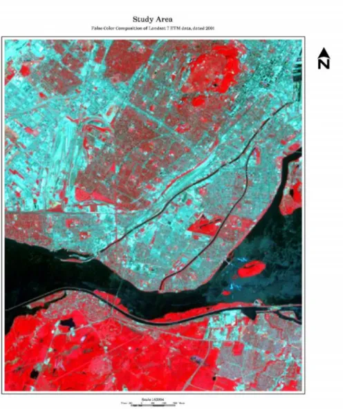
Figure 5: Study sites: site I is the entire ubanized portion of the Montreal Metropolitan Community area ; site II is the area indcated by the yellowrectangle (see Figure 6)

(43)

Figure 6: Study site – II (False color composite of 1994 LANDSAT data : red-band4, green-band 3 and blue-band 2)

Other data used in this study included the following:

1. Digital ortho-photographies (1 m spatial resolution) acquired in April, 1994. This data set was used for the evaluation the 1994 image analysis results.

2. A QUICKBIRD image (1 m resolution images) presented on Google Earth acquired in August 26th_{, 2008 used as the “ground truth” (as reference) data for evaluating the}

(44)

3. Road network database over Montreal region at scale 1: 10 000 from the government of Canada. This set of data was updated in 2003 and used to locate tie points for geo-referencing the ASTER images.

4. Digital Elevation Model (DEM) for Montreal region in 30 m resolution downloaded from government of Canada atwww.geobase.comused for the ortho-rectification of the ASTER images.

4.2 Methodological approach

The first two objectives of this study concern LANDSAT imagery and its potential for providing information on the location of changed areas as well as on the types of changes. Four change-detection techniques are examined: image differencing, CVA, PCA, and PCC. The third objective is to evaluate the impact of a finer spatial resolution (ASTER images) to the results. In order to obtain the objectives of this study, our methodological approach includes the following steps:

1. Selection of a land cover classification scheme; 2. Data preparation

3. Application of the selected change detection techniques on the LANDSAT images and accuracy assessment

4. Comparison of LANDSAT and ASTER images using the standard approach of post-classification comparison and conclusions on the impact of spatial resolution on the results These four steps are described in more details in the following paragraphs and the major procedures of this study are shown as figure 7.

(45)

Figure 7: Procedures of the study

4.2.1 Land use / land cover classification scheme

There is no a simple classification scheme of LULC which could be used with all types of imagery and all scales. As mentioned in Chapter 2 in this study the USGS scheme was chosen. Among the 9 classes of Level I (see Table 2), the following are applicable in our case: 1) Urban or Built-up Land; 2) Agriculture; 3) Rangeland; 4) Forest Land; 5) Water; 6) Wetland; and 7) Barren Land. Since only changes within the urbanized area are studied, the class “Agriculture”