HAL Id: hal-01332507
https://hal.archives-ouvertes.fr/hal-01332507
Submitted on 16 Jun 2016
HAL is a multi-disciplinary open access
archive for the deposit and dissemination of
sci-entific research documents, whether they are
pub-lished or not. The documents may come from
teaching and research institutions in France or
abroad, or from public or private research centers.
L’archive ouverte pluridisciplinaire HAL, est
destinée au dépôt et à la diffusion de documents
scientifiques de niveau recherche, publiés ou non,
émanant des établissements d’enseignement et de
recherche français ou étrangers, des laboratoires
publics ou privés.
Forecast scheduling for mobile users
Hind Zaaraoui, Zwi Altman, Eitan Altman, Tania Jimenez
To cite this version:
Hind Zaaraoui, Zwi Altman, Eitan Altman, Tania Jimenez. Forecast scheduling for mobile users. 27th
IEEE International Symposium on Personal, Indoor and Mobile Radio Commuinications (PIMRC’16),
Sep 2016, Valence, Spain. �hal-01332507�
Forecast scheduling for mobile users
Hind Zaaraoui
∗, Zwi Altman
∗, Eitan Altman
†and Tania Jimenez
‡∗Orange Labs
38/40 rue du G´en´eral Leclerc,92794 Issy-les-Moulineaux Email:{hind.zaaraoui,zwi.altman}@orange.com
†INRIA Sophia Antipolis and LINCS, France
Email:[email protected]
‡Avignon University
Email:[email protected]
Abstract—In future networks, Radio Resource Management (RRM) could benefit from Geo-Localized Measurements (GLM) thanks to the Minimization of Drive Testing (MDT) feature introduced in Long Term Evolution (LTE). Such measurements can be processed by the network and be used to optimize its
performance. The purpose of this papera is to use GLM to
significantly improve scheduling. We introduce the concept of forecast scheduler for users in high mobility that exploit GLM. It is assumed that a Radio Environment Map (REM) can provide interpolated Signal to Interference plus Noise Ratio (SINR) values along the user trajectories. The diversity in the mean SINR values of the users during a time interval of several seconds allows to achieve a significant performance gain. The forecast scheduling is formulated as a convex optimization problem namely the maximization of an α−fair utility function of the cumulated rates of the users along their trajectories. Numerical results for thee different mobility scenarios illustrate the important performance gain achievable by the forecast scheduler.
Index Terms—Forecast scheduler, alfa-fair, high mobility, Min-imizing Drive Tests, MDT, Radio Environment Maps, REM, geo-localized measurements
I. INTRODUCTION
The use of GLM for the optimization and troubleshooting of the Radio Access Network (RAN) is one of the challenging topics in future RANs. The feature that allows to perform such measurements has been introduced into the LTE standard under the term MDT. The term MDT was motivated by the need to replace costly drive tests needed to manage and to troubleshoot the network by mobile based automatic GLM. However, as is shown in this paper, GLM has the potential to be used not just for troubleshooting the RAN but for designing powerful RRM algorithms that can considerably improve the network performance.
MDT measurements can be performed in immediate or idle mode [1]. In immediate mode a connected mobile performs the GLM and immediately reports them to the Base Station (BS). In idle mode the mobile performs the measurements according to the predefined configuration (storing periodicity, logging duration, etc, and reports them to the BS once it enters a connected mode. The MDT feature is presently available in mobile chipsets but not yet activated.
The perspective of having GLM has opened an active research and development domain, namely the construction
aThis work has been partially financed by the ANR IDEFIX project.
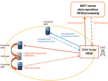
of a REM using spatial interpolation techniques ([2], [3]). The REM can be created and updated in a MDT server in the management plane and be downloaded into each BS (see Fig.1). It can provide maps for different quantities such as the received signal strength or SINR. The BS can then use the REM to optimize RRM algorithms e.g. for association, handover, or resource allocation.
Fig. 1. MDT data collection and coverage prediction
In this paper we introduce the concept of Forecast
Schedul-ingwhich is a scheduling model for users in high mobility that
uses GLM. Vehicular users are considered, and it is assumed that by means of a Global Positioning System (GPS) the users can report their location and speed to the BS. It is further
assumed that during a time windowT of the order of seconds,
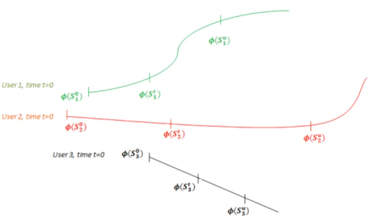
the BS can predict the SINR and data-rate variations of the users along their trajectories, e.g. using a REM. Figure 2 depicts the trajectories of three users with the corresponding data-rates. Various techniques for vehicle speed modelling and prediction have been developed, such as one related to the ARIMA model [4]; non-parametric regression [5]; Kalman filtering model [6]; or Neural Network [7].
In public transport (bus, tramway, train...), highways and trunk roads, the users trajectories are well known and can be considered as deterministic. However, trajectories may not
always be predictable, e.g. in urban environment. Previous works (e.g. [8]) developed trajectory prediction in order to manage the handoff and rerouting of connection problems. The uncertainty in the trajectory prediction can be reduced by
decreasing the time windowT , according to the environment.
Interestingly, it is shown that even for a time window of two seconds, the forecast scheduler can achieve significant performance gain.
The forecast scheduler allocation during a time windowT
is formulated as a convex optimization problem, namely the
maximization of anα−fair utility function of the cumulated
rates of the mobile users along their trajectories. Similarly to
the classical α−fair scheduling such as the Proportional Fair
(PF) [9], the forecast scheduler is an opportunistic scheduler
with a degree of fairness depending on the choice of theα−fair
parameter. However, the scheduling gain is not related to the user diversity in fast fading states (measured in a millisecond
timescale) as in classicalα−fair scheduler. In fact, vehicular
users moving with speeds of 30km/h and above experience
a too short coherence time to benefit from fast fading. The forecast scheduling gain is due to the diversity in the average SINR which is known in advance at any given time along the users’ trajectories.
The difference between the SINR predictions and the actual values is referred here as an error, and its estimation is addressed in the paper. This error may distort the forecast scheduling strategy and impact the network performances. In this paper we consider the errors due to interference variations. The idea of improving resource allocation by anticipating the future state of the mobile user has recently became an active research arena, mainly for video streaming services, see for example [10] and [11]. This research area has been denoted as anticipatory or proactive resource allocation. [12] for example develops a formulation based on Markov Decision Process (MDP) that allocates higher rates when channel deteri-oration is anticipated. The present paper considers elastic type of traffic and proposes a solution that integrates any desired
degree of fairness via theα−fair formulation. Furthermore, to
our knowledge, this is the first contribution that investigates the utilization of a REM in the design of an advanced scheduler. The paper is organized as follows. Section II describes briefly the system model. Section III presents the forecast scheduling model and its formulation as a convex optimization problem. A methodology for evaluating the impact of SINR prediction errors is addressed in Section IV. Numerical results for the evaluation of the performance of the forecast scheduler are presented in Section V followed by concluding remarks in Section VI.
II. SYSTEM MODEL
Consider an omni-directional macro-cell (BS) surrounded by six interfering neighbouring macro-cells. A Virtual Small Cell (VSC) is deployed close to the border of the cell (see Figure 3a). A VSC (also denoted as Virtual Sectorization (ViS)) is a remotely created small cell using an antenna array
that radiates a narrow beam, and can be installed beside the macro-cell antenna [13]. The purpose of considering a VSC is to create a limited area in the cell in which important SINR variations can be experienced. A single scheduler allocates resources to the macro-cell and the VSC which share the same frequency bandwidth (with no frequency reuse).
A REM is deployed in the BS and provides SINR values corresponding to the mobile location. Vehicular mobile users
with a fixed speed of50km/h are considered along one or two
trajectories. The spatial resolution of the REM is of 1m (it is
recalled that the REM interpolates GLM), and in50km/h it
corresponds to a70ms time intervals over which the SINR is
considered constant. Hence the time resolution of the forecast
scheduling is of 70ms. During this time interval, a fixed
allocation is applied, namely the same users are scheduled
at a rate depending on the technology (e.g. 1ms for LTE. The data rates are calculated from the SINR values using the Shannon formula:
φ(SIN R) = W log2(1 + SIN R), (1)
whereW is the bandwidth.
We suppose that there are no arrivals or departures of users during the scheduling duration. Full buffer users are assumed, namely having an infinite volume to transmit. The general-ization of the model to account for arrivals and departures is addressed in the next section.
III. FORECAST SCHEDULING MODEL
Consider n users moving at a constant speed during a
time interval T - the scheduling period, over which n is
considered constant. Suppose that time is in discrete space: t ∈ {1, 2, .., T } = [|1, T |] and i denotes the user number, i ∈ {1, 2, .., n} = [|1, n|]. During a scheduling period denoted here for simplicity as a unit time (e.g. 70ms), the bandwidth
is shared among the scheduled users. Letai denote the
band-width proportion allocated to a useri, ai(t) ∈ [0, 1], according
to the scheduling strategy, andW - the total bandwidth. Then
the throughput of useri is given by
aiφ(SIN Ri) = aiW log2(1 + SIN Ri), (2)
Denote byφ(St
i) the throughput of user i at time t with S
t i
being the predicted SINR. Denote byai(t) as the scheduling
allocation of the user i at time t where ∀t,Pn
i=1ai(t) = 1.
The forecast scheduling allocation policy is defined by the
following optimization problem, with α 6= 1:
maximize: f (a) = n X i=1 (PT t=1ai(t)φ(Sit))1−α 1 − α (3) with: ∀i, ∀t, ai(t) ≥ 0 and: ∀t, n X i=1 ai(t) = 1
Fig. 2. Example of 3 users with 3 different predictable trajectories.φ(St i) is
the predicted data-rate of useri at time t.
For α → 1, the optimization problem with the same
constraints reads: maximize: f (a) = n X i=1 log( T X t=1 ai(t)φ(Sit)). (4)
Both problems (3) and (4) are convex, and can be solved using powerful convex optimization solvers, e.g. CVX (see Section V for more details). The size of the optimization problem is defined by the number of unknown variables,
namelyn × T .
The formula (4) is used in this study. The interpretation of (4) is the following: resources are shared fairly among the users according to the data-rate variation in their future trajectories. For example, if a user has a coverage hole in his future trajectory, the forecast scheduler will take this into account and allocate this user as much data as possible before reaching the coverage hole while remaining fair with respect to the other users. Detailed examples are given in Section V.
In case the number of users during the intervalT changes
due to a new arrival or departure, the forecast scheduler could start from the beginning. However certain users may
have not yet been scheduled duringT , causing a problem in
the scheduler optimality. One can envisage simple heuristic approaches for handling arrival and departures. For example, the time slots scheduled for a user that leaves the network can be allocated in a Round Robin (RR) fashion to the remaining users.
One can let the number of users vary during time but in
this case the functionf in (3) should be modified to take into
account a stopping timeτ , namely the time when the users’
number varies. Denote byftthe new function to maximize in
the case where users’ number can vary. The constraints remain the same as in (3): ft(a) = E( n(t) X i=1 (Pt+τ j=tai(t)φ(Sit))1−α 1 − α ), (5)
where τ = inf{j > t, n(j) − n(j − 1) 6= 0}, and n(t) is
the number of users in the cell at timet. τ is measured from
time t. The expectation is calculated for the variable τ . The
rational of (5) is to maximize ft as long as the number of
users is fixed.
IV. SINRPREDICTION ERROR
The forecast scheduler utilizes SINR values provided by a REM. These values are averaged and depend on the in-terference level during the measurement time, which depend on the loads of the interfering cells. We expect that the dominant contribution to the difference between the actual SINR experienced by the user and the predicted value is interference. This difference is denoted as the prediction error. Example of other sources of errors include fast fading, and interpolated errors of the REM. We consider here only the error due to interference.
In order to evaluate the impact of the prediction error on the performance of the forecast scheduler, we assume an extreme (pessimistic) case: The REM provides SINR predictions for an overloaded network, i.e. the interfering cell have maximum load that equals 1. The forecast scheduler performance will be compared with that of a network with low mean load value, and is denoted as actual network. The interference in the actual network varies in time and its impact is calculated in two different ways. In the first, dynamic interference fluctuations is simulated at each scheduling iteration. In the second, the mean interference fluctuation is calculated together with the mean
distance betweenE(I) or max(I) and the random variable I
as is explained presently.
Interference modeling: We assume elastic traffic model in
which all the BS resources are allocated, even if there is just one user. A any time, a neighboring cell can have one of two states: it can be empty and produce no interference, or it has at least one user and produce maximum interference. The interference term is therefore described as follows:
I= n X i=1 1(Ni>0) Pihi rγi , (6)
where Ni is the number of users in the neighboring cell i,
Pi - the transmitted power, hi - the channel gain including
the path loss and antenna gain, andri - the distance from the
base stationi to the desired location. We rewrite 1Ni>0= Vi
whereVi is a Bernoulli random variable with parameterp
I= n X i=1 Vi Pi riγ. (7)
All theVihave the same distribution, but typically they are
not independent since each cell interferes with the other ones.
However we suppose thatVi are independent due to the small
impact on the interference estimation.p is defined as the mean
load of the cell.
We want to know how the variation of distance d
be-tween the mean E(I) or max(I) and the random variable
I impacts the forecast scheduling. We define the distance d
deviation of I, σ(I). We use the following approximation
for the SINR taking into account the interference σ(I) (if
σ(I) E(I) < 1): SIN R= P h E(I) + σ(I) ≈ P h E(I)(1 − σ(I) E(I)+ σ(I) E(I) 2 ) (8)
We estimateσ(I) empirically as following:
σ(I) = v u u t1 Z Z X z=1 (Iz−E(I))2 (9)
where Z is the number of experiments, {I1, ...IZ} - a set
of iid experiments. Eσ(I)(I) depends on the distances between a
location and neighbor BSs.
If we do not have any experience value of E(I) then we
replace it bymax(I) where we suppose that all the neighbor
cells have at least one user and interfer the principal studied cell: SIN R= P h max(I) − σm(I) ≈ P h max(I)(1+ σm(I) max(I)+ σm(I) max(I) 2 ), (10)
whereσm(I) empirically as following:
σm(I) = v u u t1 Z Z X z=1 (Iz−max(I))2 (11)
By comparing the throughput gain achieved using predicted and actual SINR values, one can estimate the impact of pre-diction error. Interestingly, one can also compare the scheduler decisions in two cases using the following formula:
error= 1 n × T X i∈users X t∈times 1{|ai(t)−aei(t)|>ǫ}, (12)
where a is the forecast scheduling strategy using the REM,
namely the predicted SINR values and ae is the forecast
scheduling strategy using measurements from the actual
net-work andǫ - the tolerated error. One can observe (see Section
V) that the two strategies provide almost identical Mean User Throughput (MUT).
V. NUMERICAL RESULTS
A. CVX resolution
The optimization problem (3) is convex. We choose in this work the CVX library implemented in Matlab to resolve this convex problem (see [14] and [15]). The CVX resolution process verifies the convexity of the problem and solves it using SDPT3 or SeDuMi. SDPT3 is a Matlab implementa-tion of infeasible path-following algorithms for solving conic programming problems whose constraint cone is a product of semidefinite cones. It uses a predictor-corrector primal-dual path-following method with different types of search direction. SeDuMi is a linear/quadratic/semidefinite solver for Matlab and Octave.
(a) Trajectory with VSC deploy-ment 0 50 100 150 200 250 300 0 50 100 150 200 250 Iteration (1 iteration = 70ms) SI N R (l in e a r) (b) SINR trajectories Fig. 3. Scenario 1 trajectories
B. Forecast scheduling gain
Consider mobile users driving at 50km/h. At this speed,
coherence time is too short to benefit from fast fading diversity and therefore a RR scheduling is used as a baseline. The forecast scheduling model using a REM for a highly loaded network (i.e. for high interference) is compared to the RR baseline scheduler. Simulation parameters including network and mobility parameters are given in Table I.
In order to assess the performance of the forecast scheduler, three scenarios of mobility are considered. They differ from one another by the degree of variation (or smoothness) of the predicted SINR along the mobile trajectories:
• Scenario 1: a VSC (fixed beam) near the cell edge is
crossed by a road with vehicular users (Figs.3a and 3b);
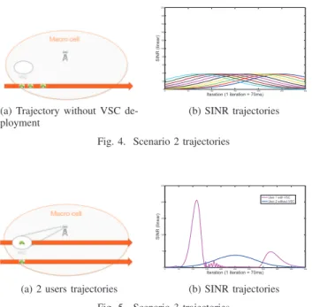
• Scenario 2: a road with vehicular users crosses the
macro-cell (no VSC, Figs.4a and 4b);
• Scenario 3: two vehicular users are considered; one user
drives along a road that traverses a VSC close to the cell edge, and the other user drives on another road without a VSC (Figs.5a and 5b).
TABLE I
NETWORK ANDTRAFFIC CHARACTERISTICS
Network parameters
Number of macro BSs 1
Number of interfering BSs 6
Macro-cell layout hexagonal omni sector
Intersite distance 500m
Bandwidth 20M Hz
Channel characteristics
Thermal noise −174dBm/Hz
Macro Path loss (d in km) 128.1 + 37.6log10(d) dB
Mobility traffic characteristics
User speed 50km/h
Number of users 10
Time between vehicles 1.4s
File sizeσ full buffer (∞)
Error toleratedǫ (eq.12) 0.05 Forecast scheduling durationT 20sec One iteration = Scheduling delay 70ms Average sliding window 15iter.
Figure 6 presents the mean user throughput gains for the three scenarios achieved by the forecast scheduler with respect to the baseline RR scheduler. As expected, the gain depends on the degree of SINR variation along the trajectories of the different scenarios. The bigger the SINR variations, the higher
(a) Trajectory without VSC de-ployment 0 50 100 150 200 250 300 0 20 40 60 80 100 120 140 160 180 200 Iteration (1 iteration = 70ms) SI N R (l in e a r) (b) SINR trajectories Fig. 4. Scenario 2 trajectories
(a) 2 users trajectories
0 50 100 150 200 250 300 350 400 450 500 0 50 100 150 200 250 Iteration (1 iteration = 70ms) SI N R (l ine a r) User 1 with VSC User 2 without VSC (b) SINR trajectories Fig. 5. Scenario 3 trajectories
is the forecast scheduling gain. The achieved gains are of 117%, 33%, 40% for scenarios 1, 2 and 3 respectively. While the throughput gain for scenario 1 is huge due to the steep SINR variations caused by VSC, it is interesting to see that significant gain can also be achieved for very moderate SINR variations of scenario 2.
With VSC (Scenario 1) 2 trajectories (Scenario 3) Without VSC (Scenario 2) 0 20% 40% 60% 80% 100% 120% 140% g a in i n % Forecast scheduling
Fig. 6. Forecast scheduling gain compared to the baseline RR scheduling for the three scenarios
C. Interference error impact
We investigate the impact of interference on the forecast scheduling for scenarios 1-3 (see Figs.3a-3b to 5a-5b). We recall that the REM data corresponds to maximal interference
(neighboring cell load of100%). We compute the error using
eq. (12)) for the three scenarios in the case where the neighbor
cells’ load is of10%. In Fig.7, one can notice that the mean
variation of the interference (formula (10)) has little impact on the scheduling strategy (red, blue and black charts). However if interference changes randomly in each iteration with average
neighbor cells’ load of 10%, the error reaches 22% for the
worst case, namely scenario 3 (green curve).
In the case of the mean variation of the interference, a
scheduling strategy error of at most 5% is observed for
scenario 1. The error for scenario 3 reaches10% for T = 2sec.
For all the scenarios, the error decreases with the increase of
the durationT of the forecast scheduling. When the scheduling
interval is too short, the SINR dynamics is likely to be limited, and the diversity in the mean SINR along the trajectory can be less exploited. In this case, the impact of interference variations on the scheduler strategy (decisions) will be higher, which explains the increase in the scheduling error for smaller T .
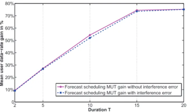
Figure 8 shows the forecast scheduling gain in MUT with respect to the baseline RR scheduler for scenario 1. The gain
increases with the scheduling duration T . The more SINR
information is available in time, the higher is the predictive scheduling gain. One can see that interference error of the REM with respect to the actual network has little impact on the schedular performance measured in terms of mean user throughput.
Figures 9 and 10 depict the normalized throughput varia-tions in time for the three strategies: Forecast scheduling with interference error, forecast scheduling without errors, and the baseline RR scheduling. One can see how the MUT varies
dynamically in time for the two extreme cases:T = 2sec and
T = 20sec for scenario 1 (with a sliding averaging window
of 1sec = 15 iterations). One can observe that the MUTs for
the forecast scheduling with and without interference error are practically the same and are almost always better than the
baseline scheduling strategy for bothT = 2s and T = 20s.
2 5 10 15 20 1% 3% 5% 7% 9% 11% 13% 15% 17% 19% 21% 23% Duration T Sc h e d u li n g s tr a te g y e rr o rs i n %
Scenario 1 mean errors Scenario 3 errors, dynamic Scenario 3 mean errors Scenario 2 mean errors
Fig. 7. Forecast scheduling strategy error in% for the three scenarios and for10% mean load of the interfering cells as a function of the scheduling intervalT .
VI. CONCLUSION
This paper has introduced the forecast scheduling which is a novel scheduling approach for users in high mobility that utilizes geo-localized measurements. Such measurements can be generated by a REM thanks to MDT data. This scheduling model consists of exploiting predicted SINR variations along the users’ trajectories and allocate resources fairly between the users during the scheduling period. The model is based on maximizing a convex utility function under constraints and
2 5 10 15 20 0 10% 20% 30% 40% 50% 60% 70% 80% Duration T Me a n u s e r d a ta −r a te g a in i n %
Forecast scheduling MUT gain without interference error Forecast scheduling MUT gain with interference error
Fig. 8. Forecast scheduling gain in MUT comparing to RR with and without interference error 0 50 100 150 200 250 300 2.5 3 3.5 4 4.5 5 5.5 6 6.5 7 7.5 Iteration (1 it. = 70 ms) MU T w ith o u t b a n d w id th fa c to r
Forecast scheduling without interference error MUT in time Forecast scheduling with interference error MUT in time RR MUT in time
Fig. 9. Time variation of the data-rate for the forecast scheduler with T=2s and the base line RR scheduler, averaged with 15 iteration sliding window
0 50 100 150 200 250 300 2 3 4 5 6 7 8 9 10 Iteration (1 it. = 70 ms) MU T w ith o u t b a n d w id th fa c to r
Forecast scheduling without interference error MUT in time Forecast scheduling with interference error MUT in time RR MUT in time
Fig. 10. Time variation of the data-rate for the forecast scheduler with T=20s and the base line RR scheduler, averaged with 15 iteration sliding window
depends on a α fairness parameter. In this study, the CVX
solver has been used to resolve this optimization problem. We have shown that the forecast scheduling model can achieve very high MUT gains compared to RR scheduling in case of high SINR variations and a long scheduling interval. The gain remains significant also for moderate SINR variations along the trajectory. Simulation scenarios have shown that errors in SINR measurements with respect to the predicted ones (e.g. from a REM) due to interference variations have
negligible impact on the obtained throughputs. Such error may distort the forecast scheduling strategy (decisions). This work is just one example of how geo-localised measurements can improve RRM and optimize the network performance. Such measurements are likely to be available thanks to the MDT capable mobiles introduced in 4G networks.
REFERENCES
[1] W. Hapsari, A. Umesh, M. Iwamura, M. Tomala, B. Gyula, B. Sebire et al., “Minimization of drive tests solution in 3GPP,” IEEE Communi-cations Magazine, vol. 50, no. 6, pp. 28–36, 2012.
[2] H. Braham, S. Ben Jemaa, B. Sayrac, G. Fort, and E. Moulines, “Coverage mapping using spatial interpolation with field measurements,” in 2014 IEEE 25th Annual International Symposium on Personal, Indoor, and Mobile Radio Communication (PIMRC). IEEE, 2014, pp. 1743– 1747.
[3] A. Galindo-Serrano et al., “Cellular coverage optimization: A radio environment map for minimization of drive tests,” in Cognitive Com-munication and Cooperative HetNet Coexistence. Springer, 2014, pp. 211–236.
[4] B. M. Williams and L. A. Hoel, “Modeling and forecasting vehicular traffic flow as a seasonal arima process: Theoretical basis and empirical results,” Journal of transportation engineering, vol. 129, no. 6, pp. 664– 672, 2003.
[5] J. You and T. J. Kim, “Empirical analysis of a travel-time forecasting model,” Geographical Analysis, vol. 39, no. 4, pp. 397–417, 2007. [6] Y.-J. Yu and M.-G. Cho, “The system for predicting the traffic flow
with the real-time traffic information,” Journal of the Korea Institute of Information and Communication Engineering, vol. 10, no. 7, pp. 1312– 1318, 2006.
[7] E.-M. Lee, J.-H. Kim, and W.-S. Yoon, “Traffic speed prediction under weekday, time, and neighboring links’ speed: back propagation neural network approach,” in Advanced Intelligent Computing Theories and Applications. With Aspects of Theoretical and Methodological Issues. Springer, 2007, pp. 626–635.
[8] T. Liu, P. Bahl, and I. Chlamtac, “Mobility modeling, location tracking, and trajectory prediction in wireless atm networks,” IEEE Journal on Selected Areas in Communications, vol. 16, no. 6, pp. 922–936, 1998. [9] R. Combes, Z. Altman, and E. Altman, “Scheduling gain for
frequency-selective Rayleigh-fading channels with application to self-organizing packet scheduling,” Performance Evaluation, Feb. 2011.
[10] N. Bui, S. Valentin, and J. Widmer, “Anticipatory quality-resource allocation for multi-user mobile video streaming,” in 2015 IEEE Confer-ence on Computer Communications Workshops (INFOCOM WKSHPS). IEEE, 2015, pp. 245–250.
[11] I. Triki, R. El-Azouzi, and M. Haddad, “Anticipating resource manage-ment and qoe provisioning for mobile video streaming,” arXiv preprint arXiv:1512.05705, 2015.
[12] W. Bao and S. Valentin, “Bitrate adaptation for mobile video streaming based on buffer and channel state,” in 2015 IEEE International Confer-ence on Communications (ICC). IEEE, 2015, pp. 3076–3081. [13] A. Tall, Z. Altman, and E. Altman, “Virtual sectorization: design and
self-optimization,” in 5th International Workshop on Self-Organizing Networks (IWSON 2015), Glasgow, Scotland, May 2015.
[14] I. CVX Research, “CVX: Matlab software for disciplined convex programming, version 2.0,” http://cvxr.com/cvx, Aug. 2012.
[15] M. Grant and S. Boyd, “Graph implementations for nonsmooth convex programs,” in Recent Advances in Learning and Control, ser. Lecture Notes in Control and Information Sciences, V. Blondel, S. Boyd, and H. Kimura, Eds. Springer-Verlag Limited, 2008, pp. 95–110.