Finding the needle in a high-dimensional haystack: Canonical correlation analysis for neuroscientists

HAL Id: hal-02541124

https://hal.archives-ouvertes.fr/hal-02541124

HAL is a multi-disciplinary open access archive for the deposit and dissemination of sci-entific research documents, whether they are pub-lished or not. The documents may come from teaching and research institutions in France or abroad, or from public or private research centers.

L’archive ouverte pluridisciplinaire HAL, est destinée au dépôt et à la diffusion de documents scientifiques de niveau recherche, publiés ou non, émanant des établissements d’enseignement et de recherche français ou étrangers, des laboratoires publics ou privés.

Finding the needle in a high-dimensional haystack:

Canonical correlation analysis for neuroscientists

Hao-Ting Wang, Jonathan Smallwood, Janaina Mourao-Miranda, Cedric Xia,

Theodore Satterthwaite, Danielle Bassett, Danilo Bzdok

To cite this version:

Hao-Ting Wang, Jonathan Smallwood, Janaina Mourao-Miranda, Cedric Xia, Theodore Satterth-waite, et al.. Finding the needle in a high-dimensional haystack: Canonical correlation analysis for neuroscientists. NeuroImage, Elsevier, 2020. �hal-02541124�

1

Finding the needle in a high-dimensional haystack:

Canonical correlation analysis for neuroscientists

Hao-Ting Wang1,2,*, Jonathan Smallwood1, Janaina Mourao-Miranda3, Cedric Huchuan Xia4, Theodore D. Satterthwaite4, Danielle S. Bassett5,6,7,8,

Danilo Bzdok9,10,11,12,13,*

1

Department of Psychology, University of York, Heslington, York, United Kingdom

2

Sackler Center for Consciousness Science, University of Sussex, Brighton, United Kingdom

3_{Centre for Medical Image Computing, Department of Computer Science, University College London, London, United Kingdom;}

Max Planck University College London Centre for Computational Psychiatry and Ageing Research, University College London, London, United Kingdom

4_{Department of Psychiatry, Perelman School of Medicine, University of Pennsylvania, Philadelphia, PA, 19104, USA} 5

Department of Bioengineering, University of Pennsylvania, Philadelphia, Pennsylvania 19104, USA

6

Department of Electrical and Systems Engineering, University of Pennsylvania, Philadelphia, Pennsylvania 19104, USA

7

Department of Neurology, Perelman School of Medicine, University of Pennsylvania, Philadelphia, PA 19104 USA

8_{Department of Physics & Astronomy, School of Arts & Sciences, University of Pennsylvania, Philadelphia, PA 19104 USA} 9_{Department of Psychiatry, Psychotherapy and Psychosomatics, RWTH Aachen University, Germany}

10

JARA-BRAIN, Jülich-Aachen Research Alliance, Germany

11

Parietal Team, INRIA, Neurospin, Bat 145, CEA Saclay, 91191, Gif-sur-Yvette, France

12

Department of Biomedical Engineering, Montreal Neurological Institute, Faculty of Medicine, McGill University, Montreal, Canada

13

Mila - Quebec Artificial Intelligence Institute

* Correspondence should be addressed to:

Hao-Ting Wang H.Wang@bsms.ac.uk

Sackler Center for Consciousness Science, University of Sussex, Brighton United Kingdom

Danilo Bzdok

danilo.bzdok@mcgill.ca

Department of Biomedical Engineering, Montreal Neurological Institute, McGill University, Montreal, Canada

Mila - Quebec Artificial Intelligence Institute

2

1 A

BSTRACT

The 21st century marks the emergence of “big data” with a rapid increase in the availability of data sets with multiple measurements. In neuroscience, brain-imaging datasets are more commonly accompanied by dozens or even hundreds of phenotypic subject descriptors on the behavioral, neural, and genomic level. The complexity of such “big data” repositories offer new opportunities and pose new challenges for systems neuroscience. Canonical correlation analysis (CCA) is a prototypical family of methods that is useful in identifying the links between variable sets from different modalities. Importantly, CCA is well suited to describing relationships across multiple sets of data and so is well suited to the analysis of big neuroscience datasets. Our primer discusses the rationale, promises, and pitfalls of CCA.

Keywords: machine learning, big data, data science, neuroscience, deep phenotyping.

3

2

INTRODUCTION

The parallel developments of large biomedical datasets and increasing computational power have opened new avenues with which to understand relationships among brain, cognition, and disease. Similar to the advent of microarrays in genetics, brain-imaging and extensive behavioral phenotyping yield datasets with tens of thousands of variables (Efron, 2010). Since the beginning of the 21st century, the improvements and availability of technologies, such as functional magnetic resonance imaging (fMRI), have made it more feasible to collect large neuroscience datasets (Poldrack and Gorgolewski, 2014). At the same time, problems in reproducing the results of key studies in neuroscience and psychology have highlighted the importance of drawing robust conclusion based on large datasets (Open Science Collaboration, 2015).

The UK Biobank, for example, is a prospective population study with 500,000 participants and comprehensive imaging data, genetic information, and environmental measures on mental disorders and other diseases (Allen et al., 2012; Miller et al., 2016). Similarly, the Human Connectome Project (van Essen et al., 2013) has recently completed brain-imaging of >1,000 young adults, with high spatial and temporal resolution, featuring approximately four hours of brain scanning per participant. Further, the Enhanced Nathan Kline Institute Rockland Sample (Nooner et al., 2012) and the Cambridge Centre for Aging and Neuroscience (Shafto et al., 2014; Taylor et al., 2017) offer cross-sectional studies (n > 700) across the lifespan (18–87 years of age) in large population samples. By providing rich datasets that include measures of brain imaging, cognitive experiments, demographics, and neuropsychological assessments, such studies can help quantify developmental trajectories in cognition as well as brain structure and function. While “deep” phenotyping and unprecedented sample sizes provide opportunities for more robust descriptions of subtle population variability, the abundance of measurement for each subject does not come without challenges.

Modern datasets often provide more variables than observations of these variable sets (Bzdok and Yeo, 2017; Smith and Nichols, 2018). In this situation, classical statistical approaches can often fail to fully capitalize on the potential of these data sets. For example, even with large samples the number of participants is often smaller than the number of brain locations that have been sampled in high-resolution brain scans. On the other hand, in datasets with a particularly high number of participants, traditional statistical approaches will identify associations that are highly statistically significant but may only account for a small fraction of the variation in the data (Miller et al., 2016; Smith and Nichols, 2018). In such scenarios, investigators who aim to exploit the full capacity of big data sets to reveal important relationships between brain, cognition and disease require techniques that are

4 better suited to the nature of their data than are many of the traditional statistical tools.

Canonical correlation analysis (CCA) is one tool that is useful in unlocking the complex relationships among many variables in large datasets. A key strength of CCA is that it can simultaneously evaluate two different sets of variables, without assuming any particular form of precedence or directionality (such as in partial least squares, cf. section 4.2). For example, CCA allows a data matrix of brain measurements (e.g., connectivity links between a set of brain regions) to be simultaneously analyzed with respect to a second data matrix of behavioral measurements (e.g., response items from various questionnaires). In other words, CCA identifies the source of common statistical associations in two high-dimensional variable sets.

CCA is a multivariate statistical method that was introduced in the 1930s (Hotelling, 1936). However, CCA is more computationally expensive than many other common analysis tools and so is only recently becoming applicable for biomedical research. Moreover, the ability to accommodate two multivariate variable sets allows the identification of patterns that describe many-to-many relations. CCA, therefore, opens interpretational opportunities that go beyond techniques that map one-to-one relations (e.g., Pearson’s correlation) or many-to-one relationships (e.g., ordinary multiple regression).

Early applications of CCA to neuroimaging data focused initially on its ability in spatial signal filtering (Cordes et al., 2012; Friman et al., 2004, 2003, 2001; Zhuang et al., 2017) and more recently on the ability to combine different imaging modalities together (see Calhoun and Sui, 2016; N. Correa et al., 2010 for review). These include functional MRI and EEG (Sui et al., 2014) and grey and white matter (Lottman et al., 2018). This work used CCA to help bring together multiple imaging modalities, a process often referred to as multi-modal fusion. However, with the recent trend towards rich phenotyping and large cohort data collection, the imaging community has also recognized the capacity for CCA to provide compact multivariate solutions to big data sets. In this context, CCA can efficiently chart links between brain, cognition, and disease (Calhoun and Sui, 2016; Hu et al., 2019; Liu and Calhoun, 2014; Marquand et al., 2017; Smith et al., 2015; Tsvetanov et al., 2016; Vatansever et al., 2017; Wang et al., 2018a; Xia et al., 2018).

In this context our conceptual primer describes how CCA can deepen understanding in fields such as cognitive neuroscience that depend on uncovering patterns in complex multi-modal datasets. We consider the computational basis behind CCA and the circumstances in which it can be useful, by considering several recent applications of CCA in studies linking brain to behavior. Next, we consider the types of conclusions that can be drawn from applications of the CCA algorithm, with a focus on the scope and limitations of applying this technique. Finally, we provide a set of practical guidelines for the implementation of CCA in scientific investigations.

5

3 M

ODELING INTUITIONS

One way to appreciate the utility of CCA is by viewing this pattern-learning algorithm as an extension of principal component analysis (PCA). This widespread matrix decomposition technique identifies a set of latent dimensions as a linear approximation of the main components of variation that underlie the information contained in the original set of observations. In other words, PCA can re-express a set of correlated variables in a smaller number of hidden factors of variation. These latent sources of variability are not always directly observable in the original measurements, but in combination explain a substantial feature of how the actual observations are organized.

PCA and other matrix-decomposition approaches have been used frequently in the domain of personality research. For example, the ‘Big Five’ describes a set of personality traits that are identified by latent patterns that are revealed when PCA is applied to how people describe other people’s time-enduring behavioral tendencies (Barrick and Mount, 1991). This approach tends to produce five reliable components that explain a substantial amount of meaningful variation in data gathered by personality assessments. A strength of a decomposition method such as PCA is that it can produce a parsimonious description of the original dataset by re-expressing it as a series of compact dimensional representations. These can also often be amenable to human interpretation (such as the concept of introversion). The ability to re-express the original data in a more compact form, therefore, has appeal both computationally and statistically (because it reduces the number of variables), and because it can also aid our interpretations of the problem space (as it did in the case of the ‘Big Five’ as main personality traits).

Although similar to PCA, CCA maximizes the linear correspondence between two sets of variables. The CCA algorithm, therefore, seeks dominant dimensions that describe shared variation across different sets of measures. In this way, CCA is particularly applicable when describing observations that bridge several levels of observation. Examples include charting correspondences between i) genetics and behavior, ii) brain and behavior, or iii) brain and genetics. In order to fully appreciate these features of CCA, it is helpful to consider how the assessment of the association between high-dimensional variable sets is achieved.

3.1

M

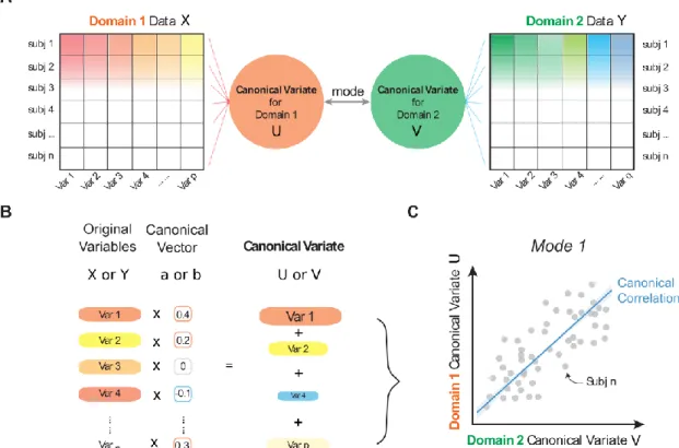
Canonical correlation analysis (Hotelling, 1936) determines the relationship between variable sets from two domains. Given and of dimensions and on the same set of observations, the first CCA mode is reflected in a linear combination of the variables in and another linear combination of the variables in

6 that maximize the first mode’s correlation

.

In addition to optimizing the correspondence between and as the first canonical mode, it is possible to continue to seek additional pairs of linear combinations that are uncorrelated with the first canonical mode(s). This process may be continued up to times. In this primer, we will refer to and as the canonical vectors, and we will refer to and as the canonical variates. The

canonical correlation denotes the correlation coefficient of the canonical variates

(see Figure 1). Let = , and , so

We can then reduce (1) to (2) subject to the constraints above.

Put differently, we define a change of basis (i.e., the coordinate system in which the data points live):

The formal relationship between canonical vectors ( and ) and canonical variates ( and ) can also be expressed as:

The relationship between the original data (X and Y) and the canonical variates U and V can be understood as the best way to rotate the left variable set and the right variable set from their original spaces to new spaces that maximize their linear correlation. The fitted parameters of CCA thus describes the rotation of the coordinate systems: the canonical vectors encapsulating how to get from the original measurement coordinate system to the new latent space, the canonical variates encoding the embedding of each data point in that new space. This coordinate system rotation is formally related to singular value decomposition (SVD). SVD is perhaps the most common means to compute CCA (Healy, 1957). Assuming X and Y are centered, the CCA solution can be obtained by applying SVD to the correlation matrix (for detailed mathematical proof, see Uurtio et al., 2017).

From a practical application perspective, there are three properties of CCA that are perhaps particularly relevant for gaining insight into the variable-rich datasets available to cognitive neuroscience: (1) joint-information compression, (2) multiplicity and (3) symmetry. We consider each of these properties in turn.

7

3.2

A key feature of CCA is that it identifies the correspondence between two sets of variables, typically capturing two different levels of observation (e.g., brain and behavior). The salient relations among each set of variables is represented as a linear combination within each domain that together reflect conjoined variation across both domains. Similar to PCA, CCA re-expresses data in form of high-dimensional linear representations (i.e., the canonical variates). Each resulting canonical variate is computed from the weighted sum of the original variable as indicated by the canonical vector. Similar to PCA, CCA aims to compress the information within the relevant data sets by maximizing the linear correspondence between the low-rank projections from each set of observations, under the constraint of uncorrelated hidden dimensions (cf. multiplicity below). This means that the canonical correlation quantifies the linear correspondence between the left and right variable sets based on Pearson’s correlation between their canonical variates; how much the right and left variable set can be considered to approach each other in a common embedding space (Fig 1). Canonical correlation, therefore, can be seen as a metric of successful joint information reduction between two variable arrays and, therefore, routinely serves as a performance measure for CCA that can be interpreted as the amount of achieved parsimony. Analogous to other multivariate modeling approaches, adding or removing even a single variable in one of the variable sets can lead to larger changes in the CCA solution (Hastie et al., 2001).

8

(A) Multiple domains of data, with p and q variables respectively, measured in the same sample of participants can be submitted to co-decomposition by CCA. The algorithm seeks to re-express the datasets as multiple pairs of canonical variates that are highly correlated with each other across subjects. Each pair of the latent embedding of the left and right variable set is often referred to as ‘mode’. (B) In each domain of data, the resulting canonical variate is composed of the weighted sum of variables by the canonical vector. (C) In a two-way CCA setting, each subject can thus be parsimoniously described two canonical variates per mode, which are maximally correlated as represented here on the scatter plot. The linear correspondence between these two canonical variates is the canonical correlation - a primary performance metric used in CCA modeling.

3.3 S

Another important feature of CCA is that the two co-analyzed variable sets can be exchanged without altering the nature of the solution. Many classical statistical approaches involve ‘independent variables’ or ‘explanatory variables’ which usually denote the model input (e.g., several questionnaire response items) as well as ‘dependent variable’ or ‘response variable’ which describes the model output (e.g., total working memory performance). However, such concepts lose their meaning in the context of CCA (Friston et al., 2008). Instead, the solutions provided by CCA reflect a description of how a unit change in one series of measurements is related to another series of measurements in another set of observations. These relationships are invariant to changes to which is the left vs. right flanking matrix to be jointly analyzed. We call this property of CCA ‘symmetry’.

The symmetry in analysis and neuroscientific interpretation produced via CCA is distinct from many other multivariate methods, in which the dependent and independent variables play distinct roles in model estimation. For instance, linear-regression-type methods account for the impact of a unit change in the (dependent) response variable as a function of the (independent) input variable. In this case, changing the dependent and independent variables can alter the nature of any specific result. A second important characteristic of CCA, therefore, is that the co-relationship between two sets of variables is determined in a symmetrical manner and describes mappings between each domain of data analyzed.

3.4 M

As third important property of CCA is that it can produce multiple pairs of canonical variates, each describing patterns of unique variation in the sets of variables. Each CCA mode carries a low-rank projection of the left variable set (one canonical variate associated with that mode) and a second linear low-rank projection of the right variables (the other canonical variate associated with that mode). After extracting the first mode, which describes the largest variation in the observed data (cf. above), CCA determines the next pair of latent dimensions whose variation

9 between both variable sets is not accounted for by the first mode. Since every new mode is found in the residual variation in the observed data, the classical formulation of CCA optimizes the modes to be mutually uncorrelated with each other, a property known as orthogonality. The use of orthogonality to constraint CCA modes is analogous to what happens using PCA. Consequently, the different modes produced by CCA are ordered by the total variation explained in the domain-domain associations. To the extent that the unfolding modes are scientifically meaningful, interpretations can afford complex data sets to be considered as being made up of multiple overlapping descriptions of the processes underlying question. For instance, much genetic variability in Europe can be jointly explained by orthogonal directions of variation along a north-south axis (i.e., one mode of variation) and a west-east axis (i.e., another mode of variation) (Moreno-Estrada et al., 2013). The ability for CCA to produce many pairs of canonical variates we refer to as ‘multiplicity’.

Figure 1 illustrates how the three core properties underlying CCA modeling and guidance of neuroscientific interpretation make it a particularly useful technique for the analysis of modern biomedical datasets – joint information compression, symmetry and multiplicity. First, CCA can provide a description that succinctly captures variation present across multiple variable sets. Second, CCA models are symmetrical in the sense that exchanging the two variable sets makes no difference to the results gained. Finally, we can estimate a collection of modes that describe the correspondence between two variable sets. As such, CCA modeling does not attempt to describe the “true” effects of any single variable (cf. below), instead targets the prominent correlation structure shared across dozens or potentially thousands of variables (Breiman and Friedman, 1997). Together these allow CCA to efficiently uncover symmetric linear relations that compactly summarize complex multivariate variable sets.

3.5 E

CCA

C

C

N

The suitability of CCA to big data sets available in modern neuroscience can be illustrated by considering examples of how it has been used to address specific questions that bear on the relationships between brain, cognition and disease. In the following section we consider 3 examples of how CCA can help describe the relationships between phenotypic measurements and neurobiological measurement such as brain activity.

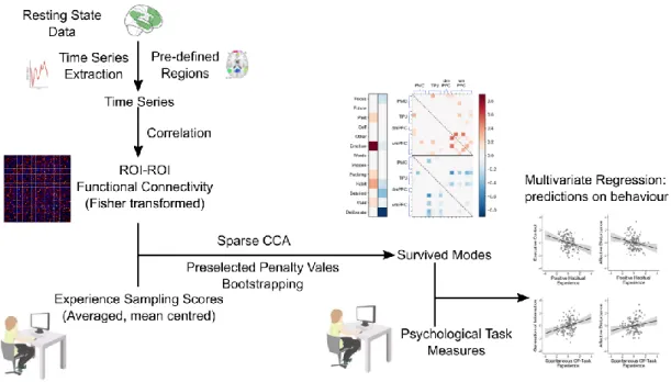
Example 1: Smith and colleagues (2015) employed CCA to uncover

brain-behavior modes of population co-variation in approximately 500 healthy participants from the Human Connectome Project (van Essen et al., 2013). These investigators aimed to discover whether specific patterns of whole-brain functional connectivity, on the one hand, are associated with specific sets of various demographics and behaviors on the other hand (see Fig 2 for the analysis pipeline). Functional brain

10 connectivity was estimated from resting state functional MRI scans measuring brain activity in the absence of a task or stimulus (Biswal et al., 1995). Independent component analysis (ICA; Beckmann et al., 2009) was used to extract 200 network nodes from fluctuations in neural activity. Next, functional connectivity matrices were calculated based on the pairwise correlation of the 200 nodes to yield a first variable set that quantified inter-individual variation in brain connectivity “fingerprints” (Finn et al., 2015). A rich set of phenotypic measures including descriptions of cognitive performance and demographic information provided a second variable set that captured inter-individual variation in behavior. The two variable arrays were submitted to CCA to gain insight into how latent dimensions of network coupling patterns present linear correspondences to latent dimensions underlying phenotypes of cognitive processing and life experience. The statistical robustness of the ensuing brain-behavior modes was determined via a non-parametric permutation approach in which the canonical correlation was the test statistic.

Smith and colleagues identified a single statistically significant CCA mode which included behavioral measures that varied along a positive-negative axis; measures of intelligence, memory, and cognition were located on the positive end of the mode, and measures of lifestyle (such as marijuana consumption) were located on the negative end of the mode. The brain regions exhibiting strongest contributions to coherent connectivity changes were reminiscent of the default mode network (Buckner et al., 2008). It is notable that prior work has provided evidence that regions composing the default mode network are associated with episodic and semantic memory, scene construction, and complex social reasoning such as theory of mind (Andrews-Hanna et al., 2010; Bzdok et al., 2012; Spreng et al., 2009). The finding of Smith and colleagues (Smith et al., 2015) provide evidence that functional connectivity in the default mode network is important for higher-level cognition and intelligent behaviors and that have important links to life satisfaction. This study illustrates the capacity of CCA for joint compression because it was able to successfully extract multivariate descriptions of data sets containing both brain measurements and a broad array of demographic and lifestyle indicators.

11

Fig 2. The analysis pipeline of Smith et al., 2015.

These investigators aimed to discover whether specific patterns of whole-brain functional connectivity, on the one hand, are associated with specific sets of correlated demographics and behaviors on the other hand. The two domains of the input variables were transformed into principle components before the CCA model evaluation. The significant mode was determined by permutation tests. The finding of Smith and colleagues (2015) provide evidence that functional connectivity in the default mode network is important for higher-level cognition and intelligent behaviors and are closely linked to positive life satisfaction.

Example 2: Another use of CCA has been to help understand the complex

relationship between neural function and patterns of ongoing thought. In both the laboratory and in daily life, ongoing thought can often shift from the task at hand to other personally relevant characteristics - a phenomenon that is often referred to by the term ‘mind-wandering’ (Seli et al., 2018). Studies suggest there is a complex pattern of positive and negative associations between states of mind-wandering(Mooneyham and Schooler, 2013). This apparent complexity raises the possibility that mind-wandering is a heterogeneous rather than homogeneous state.

Wang and colleagues (2018b) used CCA to empirically explore this question by examining the links between connectivity within the default mode network and patterns of ongoing self-generated thought recorded in the lab (Fig 3). Their analysis used patterns of functional connectivity within the default mode network as one set of observations, and patterns of self-reported descriptions recorded in the laboratory across multiple days as the second set of observations (Witten et al., 2009). The connectivity among 16 regions in the default mode network and 13 self-reported aspects on mind-wandering experience were fed into a sparse version of CCA (see Section 4.2 for further information on this variant of CCA). This analysis found two modes, one describing a pattern of positive-habitual thoughts, and a second that reflected spontaneous task-unrelated thoughts and both were

12 associated with unique patterns of connectivity fluctuations within the default mode network. As a means to further validate the extracted brain-behavior modes in new data, follow-up analyses confirmed that the modes were uniquely related to aspects of cognition, such as executive control and the ability to generate information in a creative fashion, and the modes also independently distinguished well-being measures. These data suggest that the default mode network can contribute to ongoing thought in multiple ways, each with unique behavioral associations and underlying neural activity combinations. By demonstrating evidence for multiple brain-experience relationships within the default mode network, the authors (2018b) underline that greater specificity is needed when considering the links between brain activity and neural experience (see also Seli et al., 2018). This study illustrates the property of CCA for multiplicity because it was able to identify multiple different patterns of thought each of which could be validated based on their associations with other sets of observations.

Fig 3. The analysis pipeline of Wang et al., 2018b.

Wang and colleagues (2018b) used CCA to interrogate the hypothesis that various distinct aspects of ongoing thought can track distinct components of functional connectivity patterns within the default mode network. Sparse CCA was used to perform feature selection simultaneously with the model fitting on the brain-experience data. The identified CCA modes showed robust trait combinations of positive-habitual thoughts and spontaneous task-unrelated thoughts with linked patterns of connectivity fluctuations within the default mode network. The two modes were also related to distinct high-level cognitive profiles respectively.

Example 3: In the final example, Xia and colleagues (2018, see Fig 4) mapped

item-level psychiatric symptoms to brain connectivity patterns in brain networks using resting-state fMRI scans in a sample of roughly 1000 subjects from the Philadelphia Neurodevelopmental Cohort. Recognizing the marked level of

13 heterogeneity and comorbidity in existing diagnostic psychiatric diagnoses, these investigators were interested in how functional connectivity and individual symptoms can form linked dimensions of psychopathology and brain networks (Insel and Cuthbert, 2015). Notably, the study used a feature-selection step based on median absolute deviation to first reduce the dimensionality of the connectivity feature space prior to running CCA. As a result, about 3000 functional edges and 111 symptom items were analyzed in conjunction. As the number of features was still greater than the number of subjects, sparse CCA was used (Witten et al., 2009). This variant of the CCA family penalizes the number of features selected by the final CCA model. Based on covariation-explained and subsequent permutation testing (Mišić et al., 2016), the analysis identified four linked dimensions of psychopathology and functional brain connectivity – mood, psychosis, fear, and externalizing behavior. Through a resampling procedure that conducted sparse CCA in different subsets of the data, the study identified stable clinical and connectional signatures that consistently contributed to each of the four modes. The resultant dimensions were relatively consistent with existing clinical diagnoses, but additionally cut across diagnostic boundaries to a significant degree. Furthermore, each of these dimensions were associated with a unique pattern of abnormal connectivity. However, a loss of network segregation was common to all dimensions, particularly between executive networks and the default mode network. As network segregation is a normative feature of network development, loss of network segregation across all dimensions suggests that common neurodevelopmental abnormalities may be important for a wide range of psychiatric symptoms. Taking advantage of CCA’s ability to capture common sources of variation in more than one datasets, these findings support the idea behind NIMH Research Domain Criteria that specific circuit-level abnormalities in the brain’s functional network architecture may give rise to a diverse psychiatric symptoms (Cuthbert and Insel, 2013). This study illustrates the flexible use of CCA to reveal trans-diagnostic, continuous symptom dimensions based on whole-brain intrinsic connectivity fingerprints that can cut across existing disease boundaries in clinical neuroscience.

14

Fig 4. The analysis pipeline of Xia et al., 2018.

Xia and colleagues (2018) were interested in how functional connectivity and individual symptoms can form linked dimensions of psychopathology and brain networks. The study took a feature selection step based on median absolute deviation in preprocessing to first reduce the dimensionality of the functional connectivity measures. A sparse variation of CCA was applied to extract modes of linked dimensions of psychopathology and functional brain connectivity. Based on covariation-explained and subsequent permutation testing, the analysis identified four linked dimensions – mood, psychosis, fear, and externalizing behavior – each were associated with a unique pattern of abnormal brain connectivity. The results suggested that specific circuit-level abnormalities in the brain’s functional network architecture may give rise to diverse psychiatric symptoms.

Example 4: Hu and colleagues (2018) demonstrated the successful application

of sparse multiple CCA (Witten and Tibshirani, 2009) to imaging epigenomics data of Schizophrenia. The multivariate nature of CCA is beneficial in extending our understanding of complex disease mechanism such as reflected by gene expressions, on the one hand, and high-content measurements of the brain, on the other hand. Epigenetics can be characterized into heterogeneous biological processes based on single nucleotide polymorphisms (SNPs), mRNA sequencing and DNA methylation to the primary tissue or organ level changes in the brain. The complex interplay of different genetic features affects gene expression on the regulation system of gene expression in tissues and biological structure of DNA. Combined with neuroimaging data, this exciting new avenue to chart brain-genetics relationships is an expanding field of interest in complex brain related diseases. In particular, sparse multiple CCA finds correlations across three or more domains of variables hence a good tool for exploring genetics and imaging data. This seminal multi-scale investigation proposed an adaptively reweighted sparse multiple CCA based on the conventional sparse multiple CCA proposed by Witten et al (2009). However, the conventional SMCCA is likely to overlook smaller pairwise covariance’s and/or over-considerate of omics

15 data with larger covariances. The referred study therefore proposed an enhanced algorithm variant to relieve the unfair combination by introducing weights coefficients in an adaptive manner. The adapted SMCCA was applied to schizophrenia subjects as an example. The multi-view analysis combined two genetic measures, genomic profiles from 9273 DNA methylation sites and genetic profiles from 777365 SNPs loci, for joint consideration with brain activity from resting state fMRI data across 116 anatomical regions based on the AAL brain atlas (Tzourio-Mazoyer et al., 2002). The model hyper-parameter was selected with a 5-fold cross validation. The total samples were divided into 5 subgroups, and during each fit-evaluate step, the authors picked up one subgroup as testing sample and use the rest 4 subgroups as training sample set. A score quantifying fitting success was determined by the difference between the correlation of training sample and that of the test sample, which was used in this particular study to evaluate the performance of selecting the sparsity parameters. After the sparsity parameters are selected based on the data, a bootstrapping stability selection (Meinshausen and Bühlmann, 2010) approach was used to select a stable subset of variables that most commonly occurred among the 200 bootstrapped samples. The frequency cutoff was set to be 0.6 based on Meinshausen and Bühlmann’s work (2010). The new algorithmic methodology revealed consistent brain regions and genetic variants with the past studies, such as (i) hippocampus and fusiform in the fMRI data (Kircher and Thienel, 2005), (ii) SNPs related to brain development including BSX that has influence on methylation level (Park et al., 2007), PFTK1, which is relevant to brain degenerative diseases gene THR (Shibusawa et al., 2008), and AMIGO2 which is associated with hippocampus (Laeremans et al., 2013), and (iii) neuro tube development pathway in DNA methylation that is relevant to brain development (Kamburov et al., 2013). The overall experiment has readily showcased the elegant data fusion in an multi-omics application to epigenetics and brain imaging integration. The ensuing discoveries in primary biology can provide important new perspectives on complex diseases, such as schizophrenia, with potential applications to other brain-genetics associated.

4 I

NTERPRETATION

A

ND

L

IMITATIONS OF

CCA

The goal of CCA to achieve a common decomposition of multiple matrices makes this modeling tool particularly useful for getting a handle on richly sampled descriptions of a population with observations that cross multiple levels of investigation. However, it remains a matter of ongoing debate whether this analysis technique corresponds more closely to a descriptive re-expression of the data (i.e., unsupervised modeling) or should be more readily understood as a form of

predictive reduced-rank regression (i.e., supervised modeling, cf. Bach and Jordan,

2005; Breiman and Friedman, 1997; Witten et al., 2009). There are legitimate arguments in support of both views. A supervised algorithm depends on a

16 designated modeling target to be predicted from an array of input variables, whereas an unsupervised algorithm aims to extract coherent patterns in observations without associated ground-truth labels that can be used during model estimation (Hastie et al., 2001). It is possible that as the dimensionality of one of the variable sets declines to approach the single output of most linear-regression-type methods, in which case CCA may be more similar to a more supervised modeling approach. Conversely, with increasingly large variable sets on both sides, applying CCA is perhaps closer in spirit to an unsupervised modeling approach.

Whether the investigator considers CCA as either a supervised or unsupervised method has a consequence for both the interpretation of the results and their choice of eligible strategies to validate the model solutions. For example, cross-validation is a technique that is commonly used for supervised model evaluation by comparing model-derived predictions in unseen data. In an unsupervised setting, however, there is typically no unambiguous criterion for optimization (such as low residual sum of squares in supervised linear regression) that could be used for model selection or model evaluation, such as in cross-validation schemes (Hastie et al., 2001). However, cross validation is seldom used to buttress unsupervised model solutions, such as clustering methods like k-means or matrix decomposition techniques like PCA, because in these cases there is often no label upon which to evaluate performance (Bzdok, 2017; Hastie et al., 2001; Pereira et al., 2009). In situations when a CCA model describes the data without a known quantity to be predicted, cross-validation procedures can evaluate a CCA model by projecting data from new, previously unseen individuals using the canonical vectors observed from the initial sample. If this is not possible, an alternative validation strategy is to demonstrate whether the canonical variates of the obtained CCA solution are useful in capturing variation in other unseen measurements in the same set of individuals (e.g. Wang et al., 2018a). Yet another validation strategy for CCA is to show that the solutions it produces are robust when repeating the analysis on random subsets of the (already seen) individuals in so-called split-half analyses (Miller et al., 2016; Smith et al., 2015).

From a formal perspective, the optimization objective governing parameter estimation during CCA fitting is unusual for a supervised model because it is based on Pearson’s correlation metric. The majority of linear-regression-type predictive models have an optimization function that describes the degree of deviation from the ground-truth labels, including different residual-sum-of-squares loss functions (Casella and Berger, 2002; Hastie et al., 2001). Moreover, the symmetry of the variable sets in CCA is another reason why CCA may be considered an example of an unsupervised analysis tool. We are not aware of any existing supervised predictive model that would yield identical sets of model parameter fits after the independent and dependent variables have been swapped (if possible). To conclude, the CCA

17 model is a relatively unique approach that shares features of what are classically features of both supervised and unsupervised methods.

Another way to categorize statistical methods is based on their modeling goal:

estimation, prediction, or inference (Efron and Hastie, 2016; Hastie and Tibshirani,

1990). Model estimation refers to the process of adjusting randomly initialized parameters by fitting them to the data at hand; an intuitive example of these are beta parameters in classical linear regression. As model estimation can often be performed without applying the model to unseen observations or assessing the fundamental trueness of the effects, some authors recently called this modeling regime “retrodiction” (McElreath, 2015; Pearl and Mackenzie, 2018). Prediction is concerned with maximizing model fit in terms of optimizing its usefulness for predicting unseen data in the future. Finally, drawing inferences on model fits has frequently been based on statistical null hypothesis testing and accompanying methodology (Wasserstein and Lazar, 2016). This form of drawing rigorous conclusions from data is especially useful in the classical analysis paradigm where the primary goal is to make precise statements about the contribution of single input variables.

In the context of this tripartite view of general modeling goals, CCA most naturally qualifies for the estimation category, rather than either primarily a predictive or inferential tool. Because of its exploratory nature, CCA can often be useful for applications focused on uncovering parsimonious structure in complex high-dimensional spaces as alternative descriptions of the observations at hand. Identifying the predictive value of individual variables in new data is not an integral part of the optimization objective underlying CCA. In fact, CCA applications often do not seek to establish statistically significant links between subsets of the variables in each set, because the analytic goal is targeted at relevant patterns found across the entirety of both variable arrays. Even if p-values are obtained based on non-parametric null hypothesis testing in the context of CCA, the particular null hypothesis at play (commonly: the left and right variable matrix carry no corresponding information) is really centered on the overall robustness of the latent space correlations, as measured by the canonical correlations between the (projected) variable sets, and is not centered on specific single measurements; let alone on any particular link between one measurements from the left and one measurements from the right variable set. Thus, using CCA to pinpoint specific relations should only be done in a cautious manner. Stated in another way, CCA is not an optimal choice when the investigator wishes to make strong statements about the relevance and relationships of individual variables of the interrogated within a variable sets - a property shared with many other pattern-learning tools.

18

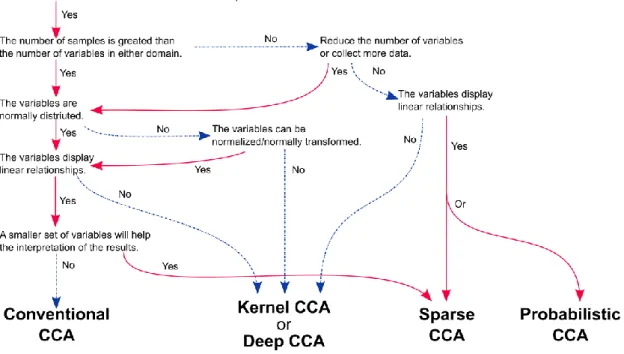
4.1

Having considered the relationship between CCA and existing classifications of statistical techniques, we next consider some of the challenges that researchers may encounter when considering whether CCA is a good choice for a given data-analysis problem. We summarize the choices that a researcher is faced with in the form of a flowchart (see Fig 5). As with many statistical approaches, the number of observations n in relation to the number of variables p is a key aspect when considering whether CCA is likely to be useful (Giraud, 2014; Hastie et al., 2015). Ordinary CCA can only be expected to yield useful model fits in data with more observations than the number of variables of the larger variable set (i.e., ). Concretely, if the number of individuals included in the analysis is too close to the number of brain or behavior or genomics variables, then CCA will struggle to approximate the latent dimensions in the population (but see regularized CCA variants below). In these circumstances, even if CCA reaches a solution, without throwing an error, the derived canonical vectors can be meaningless (Hastie et al., 2015). More formally, in such degenerate cases, CCA loses its ability to find unique identifiable solutions (despite being a non-convex optimization problem) that another laboratory with the same data and CCA implementation could also obtain (Jordan, 2018). Additionally, as an important note on reproducibility, with increasing number of variables in one or both sets, the ensuing canonical correlation often tends to increase due to higher degrees of freedom. An importance consequence is that the canonical correlations obtained from CCA applications with differently sized variables sets cannot be directly used to decide which of the obtained CCA models are “better”. The CCA solution is constraint by the sample as well as the number of variables. As a cautionary note, the canonical correlation effect sizes obtained from the training data limit statements about how the obtained CCA solution at hand would perform on future or other data.

In a similar vein, smaller datasets offering measurements from only a few dozen individuals or observations may have difficulty in fully profiting from the strengths of multivariate procedure such as CCA. Moreover, the ground-truth effects in areas like psychology, neuroscience, and genetics are often small, which are hard to detect with insufficient sampling of the variability components. One practical remedy that can alleviate modeling challenges in small datasets is using data reduction methods such as PCA or other data-reduction method for preprocessing each variable before applying CCA (e.g. Smith et al., 2015) or to adopt a sparse variant of CCA (see below). Reducing the variable sets according to their most important directions of linear variation can facilitate the CCA approach and the ensuing solution, including canonical variates, can be translated back to and interpreted within the original variable space. These considerations illustrate why

19 CCA applications have long been less attractive in the context of many neuroscience studies, while its appeal and feasibility are now steadily growing as evermore rich, multi-modal, and open datasets become available (Davis et al., 2014).

A second limitation concerns the scope of the statistical relationships that CCA can discover and quantify in the underlying data. As a linear model, classical CCA imposes the assumption of additivity on the underlying relationships to unearth relevant linked co-variation patterns, thus ignoring more complicated variable-variable interactions that may exist in the data. CCA can accommodate any metric variable without strict dependence on normality. However, Gaussian normality in the data is desirable because CCA exactly operates on differences in averages and spreads that parameterize this data distribution. Before CCA is applied to the data, it is common practice that one evaluates the normality of the variable sets and possibly apply data an appropriate transformation, such as z-scoring (variable normalization by mean centering to zero and unit-spread scaling to one) or Box-Cox transformations (variable normalization involving logarithm and square-root operations). Finally, the relationships discovered by CCA solutions have been optimized to highlight those variables whose low-dimensional projection is most (linearly) coupled with the low-dimensional projection of the other variable set. As such, the derived canonical modes provide only one window into which multivariate relationships are most important given the presence of the other variable set, rather than identifying variable subsets that are important in the dataset per se.

Fig 5. A flowchart illustrating the choices when considering the application of CCA a dataset.

This flowchart summarizes some of the decision choices faced by a researcher when considering whether to use CCA to analyze her data. Note some of the choices of CCA variation depend on the interpretative context (i.e. conventional vs sparse CCA and sparse CCA vs probabilistic CCA).

20

4.2

CCA is probably the most general statistical approach to distill the relationships between two high-dimensional sources of quantitative measurements. In fact, CCA can be viewed as a broad class of methods that generalizes many more specialized approaches from the general linear model (GLM Gelman and Hill, 2007). In fact, most of the linear models commonly used by behavioral scientists for parametric testing (including ANOVA, MANOVA, multiple regression, Pearson’s correlation, and t-test) can be interpreted as special cases of CCA (Knapp, 1978; Thompson, 2015). Because these techniques are closely related, when evaluating CCA it will often be beneficial to more deeply understand the opportunities and challenges of similar approaches. Related methods:

i) PCA has certain similarities to CCA, although PCA performs unsupervised matrix decomposition of one variable set (Shlens, 2014a). A shared property of PCA and CCA is the orthogonality constraint imposed during structure discovery. As such, the set of uncovered sources of variation (i.e., modes) are assumed to be uncorrelated with each other in both methods. As an important difference, there are PCA formulations that minimize the reconstruction error between the original variable set and the back-projection of each observation from the latent dimensions of variation (Hastie et al., 2015). CCA instead directly optimizes the correspondence between the latent dimensions directly in the embedding space, rather than the reconstruction loss in the original variables incurred by the low-rank bottleneck. Moreover, PCA can be used for dimensionality reduction as a pre-processing step before CCA (e.g. Smith et al., 2015). ii) Analogous to PCA and CCA, independent component analysis (ICA) also extracts hidden

dimensions of variation in a potentially high-dimensional variable sets. While CCA is concerned with revealing multivariate sources of variation based on linear covariation structure, ICA can identify more complicated non-linear relationships in data that can capture statistical relationships that go beyond differences in averages and spreads (Shlens, 2014b). A second aspect that departs from CCA is the fact that latent dimensions obtained from ICA are not naturally ordered from highest to lowest contribution in reducing the reconstruction error, which needs to be computed in a later step. Another difference between CCA and ICA is how both approaches attempt to identify solutions featuring a form of uncorrelatedness. As described earlier, CCA’s uses the constraint of orthogonality to obtain uncorrelated latent dimensions; in contrast, ICA optimizes the independence between the emerging hidden sources of variation. In this context independence between two variables implies their uncorrelatedness, but the lack of a linear correlation between the two variables does not ensure the lack of a nonlinear statistical relation between the two variables. Finally, it is worth mentioning that ICA can also be used as a post-processing step to further inspect effects in CCA solutions (Miller et al., 2016; Sui et al., 2010).

iii) Partial least squares (PLS) regression is more similar to CCA than PCA or ICA. This is because PLS and CCA can identify latent dimensions of variation across two variable sets (McIntosh et al., 1996). A key distinctive feature of PLS is that the optimization goal

21 is to minimize the covariance rather than the linear correlation. As such, the relationship between PLS and CCA can be more formally expressed as:

.

While PLS is consistently viewed and used as a supervised method, it is controversial whether CCA should counted as part of the supervised or unsupervised family (see above)(Hastie et al., 2001). Further, many PLS and CCA implementations are similar in the sense that they impose an orthogonality constraint on the hidden sources of variation to be discovered. However, the two methods are also different in the optimization objective in the following sense: PLS maximizes the variance of the projected dimensions with the original variables of the designed response variables. Instead, CCA operates only in the embedding spaces of the left and right variable sets to maximize the correlation between the emerging low-rank projections, without correlation any of the original measurements directly. CCA thus indirectly identifies those canonical vectors whose ensuing canonical variates correlate most. In contrast to CCA, PLS is scale-variant (by reliance on the covariance), which leads to different results after transforming the variables.

As well as considering the alternative methods, there are also a number of important extensions to the CCA model, each of which are optimized with respect to specific analytic situations. These different model extension are presented at the foot of Figure 5.

Model extensions:

i. Probabilistic CCA is a modification that motivates classical CCA as a generative model (Bach and Jordan, 2005; Klami et al., 2013). One advantage of this CCA variant is that it has a more principled definition of the variation to be expected in the data and so has more opportunity to produce synthetic but plausible observations once the model has been fit. Additionally, because probabilistic CCA allows for the introduction of prior knowledge into the model specification, an advantageous aspect of many Bayesian models, this approach has been shown to yield more convincing results in small biomedical datasets which would otherwise be challenging to handle using ordinary CCA (e.g. Fujiwara et al., 2009; Huopaniemi et al., 2009).

ii. Sparse CCA (SCCA Witten et al., 2009) is a variant for identifying parsimonious sources of variation by encouraging exactly-zero contributions from many variables in each variable set. Besides facilitating interpretation of CCA solutions, the imposed -norm penalty term is also effective in scaling CCA applications to higher-dimensional variable sets, where the number of variables can exceed the number of available observations (Hastie et al., 2015). One consequence of the introduction of the sparsity constraint is that it can interfere with the orthogonality constraint of CCA. In neuroscience applications, the sparser the CCA modes that are generated, the more the canonical variates of the different modes can be correlated with one another. Additionally, it is important to note that the variation that each mode explains will not decrease in order from the first mode onwards as occurs in ordinary

22 CCA. As a side node, other regularization schemes can also be an interesting extension to classical CCA. In particular, imposing an -norm penalty term stabilizes CCA estimation in the wide-data setting using variable shrinkage, without the variable-selection property of the sparsity-inducing constraint (Witten and Tibshirani, 2009).

iii. Multiset CCA (Parra, 2018) or multi-omics data fusion (Hu et al., 2018) expend the analysis for more than two domains of data. In the field of neuroimaging, the application of multiset CCA is common blind source separation among subjects or among multiple imaging features (e.g. fMRI, structural MRI, and EEG). The advantage of multiset CCA is the flexibility in addressing variability in each domain of data without projecting data into a common space (c.f. ICA). The sparse variation of multiset CCA is also a popular choice to overcome the limitations when handling high number of variables. Discriminative CCA, or Collaborative Regression (Gross and Tibshirani, 2015; Luo et al., 2016), is a form of multiset sparse CCA (Hu et al., 2018; Witten and Tibshirani, 2009). In discriminative CCA, one data domain is a vector of labels. The labels help identify label/phenotype related cross-data associations in the other two domains, hence created a supervised version of CCA.

iv. Kernel CCA (KCCA; Hardoon et al., 2004) is an extension of CCA designed to capture more complicated nonlinear relationships. Kernels are mapping functions that implicitly express the variable sets in richer feature spaces, without ever having to explicitly compute the mapping, a method known as the ‘kernel trick’ (Hastie et al., 2001). KCCA first projects the data into this enriched virtual variable space before performing CCA in that enriched input space. It is advantageous that KCCA allows for the detection of complicated non-linear relationships in the data. The drawback is that the interpretation of variable contributions in the original variable space is typically more challenging and in certain cases impossible. Further, KCCA is a nonparametric method; hence, the quality of the model fit scales poorly with the size of the training set.

v. Deep CCA (DCCA Andrew et al., 2013) is a variant of CCA that capitalizes on recent advances in “deep” neural-network algorithms (Jordan and Mitchell, 2015; LeCun et al., 2015). A core property of many modern neural network architectures is the capacity to learn representations in the data that emerge through multiple nested non-linear transformations. By analogy, DCCA simultaneously learns two deep neural network mappings of the two variable sets to maximize the correlation of their (potentially highly abstract) latent dimensions, which may remain opaque to human intuition.

5 P

RACTICAL CONSIDERATIONS

After these conceptual considerations, we next consider the implementation of CCA. The computation of CCA solutions is possible by built-in libraries in MATLAB (canocorr), R (cancor or the PMA package), and the Python machine-learning library scikit-learn (sklearn.cross_decomposition.CCA). The sparse CCA mentioned in the examples is implemented in R package PMA. These code implementations provide

23 comprehensive documentation for how to deploy CCA. For readers interested in reading more on detailed technical comparisons and discussions of CCA variants, please refer to the texts in Table 1.

Table 1. Further reading on variations of CCA

Fusion CCA Calhoun, V.D., Sui, J., (2016). Multimodal Fusion of Brain Imaging Data: A Key to

Finding the Missing Link(s) in Complex Mental Illness. Biol. Psychiatry Cogn. Neurosci. Neuroimaging 1, 230-244.

Correa, N.M., Adali, T., Li, Y., Calhoun, V.D., (2010). Canonical Correlation Analysis for Data Fusion and Group Inferences. IEEE Signal Process Mag 27, 39-50.

Sui, J., Castro, E., He, H., Bridwell, D., Du, Y., Pearlson, G.D., Jiang, T., Calhoun, V.D., (2014). Combination of FMRI-SMRI-EEG data improves discrimination of

schizophrenia patients by ensemble feature selection. Conf. Proc. ... Annu. Int. Conf. IEEE Eng. Med. Biol. Soc. IEEE Eng. Med. Biol. Soc. Annu. Conf. 2014, 3889-3892.

CCA application to signal processing

Cordes, D., Jin, M., Curran, T., Nandy, R., (2012). Optimizing the performance of local canonical correlation analysis in fMRI using spatial constraints. Hum. Brain Mapp. 33, 2611-2626.

Friman, O., Borga, M., Lundberg, P., Knutsson, H., (2003). Adaptive analysis of fMRI data. Neuroimage 19, 837-845.

Friman, O., Borga, M., Lundberg, P., Knutsson, H., (2002). Detection of neural activity in fMRI using maximum correlation modeling. Neuroimage 15, 386-395. Friman, O., Cedefamn, J., Lundberg, P., Borga, M., Knutsson, H., (2001). Detection of neural activity in functional MRI using canonical correlation analysis. Magn. Reson. Med. 45, 323-330.

Lottman, K.K., White, D.M., Kraguljac, N. V., Reid, M.A., Calhoun, V.D., Catao, F., Lahti, A.C., (2018). Four-way multimodal fusion of 7 T imaging data using an mCCA+jICA model in first-episode schizophrenia. Hum. Brain Mapp. 1-14. Yang, Z., Zhuang, X., Sreenivasan, K., Mishra, V., Curran, T., Byrd, R., Nandy, R., Cordes, D., (2018). 3D spatially-adaptive canonical correlation analysis: Local and global methods. Neuroimage 169, 240-255.

Zhuang, X., Yang, Z., Curran, T., Byrd, R., Nandy, R., Cordes, D. (2017). A Family of Constrained CCA Models for Detecting Activation Patterns in fMRI. NeuroImage, 149:63-84.

Multipe CCA / Multi-omics data fusion

Correa, N.M., Eichele, T., Adali, T., Li, Y.-O., Calhoun, V.D., (2010). Multi-set canonical correlation analysis for the fusion of concurrent single trial ERP and functional MRI. Neuroimage 50, 1438-45. doi:10.1016/j.neuroimage.2010.01.062 Hu, W., Lin, D., Cao, S., Liu, J., Chen, J., Calhoun, V.D., Wang, Y., (2018). Adaptive Sparse Multiple Canonical Correlation Analysis With Application to Imaging (Epi)Genomics Study of Schizophrenia. IEEE Trans. Biomed. Eng. 65, 390–399. https://doi.org/10.1109/TBME.2017.2771483

24

CCA vs multivariate methods

Hair, J.F., Black, W.C., Babin, B.J., Anderson, R.E., (2010). Multivariate data analysis, 7th editio. Ed.

Le Floch, É., Guillemot, V., Frouin, V., Pinel, P., Lalanne, C., Trinchera, L., Tenenhaus, A., Moreno, A., Zilbovicius, M., Bourgeron, T., Dehaene, S., Thirion, B., Poline, J.-B., Duchesnay, É., (2012). Significant correlation between a set of genetic

polymorphisms and a functional brain network revealed by feature selection and sparse Partial Least Squares. Neuroimage 63, 11-24.

doi:10.1016/j.neuroimage.2012.06.061

Liu, J., Calhoun, V.D., (2014). A review of multivariate analyses in imaging genetics. Front. Neuroinform. 8, 29. doi:10.3389/fninf.2014.00029

Parra, L.C., (2018). Multiset Canonical Correlation Analysis simply explained. Arxiv. Pituch, K.A., Stevens, J.P., (2015). Applied multivariate statistics for the social sciences: Analyses with SAS and IBM’s SPSS, Routledge.

https://doi.org/10.1017/CBO9781107415324.004

Sui, J., Adali, T., Yu, Q., Chen, J., Calhoun, V.D., (Sui et al., 2012). A review of multivariate methods for multimodal fusion of brain imaging data. J. Neurosci. Methods 204, 68-81. doi:10.1016/j.jneumeth.2011.10.031

CCA vs PLS Grellmann, C., Bitzer, S., Neumann, J., Westlye, L.T., Andreassen, O.A., Villringer, A., Horstmann, A., (2015). Comparison of variants of canonical correlation analysis and partial least squares for combined analysis of MRI and genetic data. Neuroimage 107, 289-310. doi:10.1016/j.neuroimage.2014.12.025

Sun, L., Ji, S., Yu, S., Ye, J., (2009). On the equivalence between canonical

correlation analysis and orthonormalized partial least squares. Proc. 21st Int. jont Conf. Artifical Intell.

Uurtio, V., Monteiro, J.M., Kandola, J., Shawe-Taylor, J., Fernandez-Reyes, D., Rousu, J., (2017). A Tutorial on Canonical Correlation Methods. ACM Comput. Surv. 50, 1-33. doi:10.1145/3136624

5.1 P

Some minimal data preprocessing is usually required as for most machine-learning methods. CCA is scale-invariant in that standardizing the data should not change the resulting canonical correlations. This property is inherited from Pearson’s correlation defined by the degree of simultaneous unit change between two variables, with implicit standardization of the data. Nevertheless, z-scoring of each variable of the measurement sets is still recommended before performing CCA to facilitate the model estimation process and to enhance interpretability. To avoid outliers skewing CCA estimation, it is recommended that one applies outlier detection and other common data-cleaning techniques (Gelman and Hill, 2007). Several readily applicable heuristics exist to identify unlikely variable values, such as

25 replacing extreme values with 5th and 95th percentiles of the respective input dimension, a statistical transformation known as ‘winsorizing’. Missing data is a common occurrence in large dataset. It is recommended to exclude observations with too many missing variables (e.g. those missing a whole domain of a questionnaire). Alternatively, missing variables can be “filled in” with mean or median when the proportion of missing data is small, or more sophisticated data-imputation techniques.

Besides unwarranted extreme and missing values, it is often necessary to account for potential nuisance influences on the variable sets. Deconfounding procedures are a preprocessing step in many neuroimaging data analysis settings to reduce the risk of finding non-meaningful modes of variation (such as motion). The same procedures that are commonly applied prior to the use of linear-regression analyses can also be useful in the context of CCA. Note that deconfounding is typically performed as an independent preceding step because the CCA model itself has no explicit noise component. Deconfounding is often carried by creating a regression model that captures the variation in the original data that can be explained by the confounder. The residuals of such regression modeling will be the new “cleaned” data with potential confound information removed. In neuroimaging, for example, head motion, age, sex, and total brain volume have frequently been considered unwanted sources of influence in many analysis contexts (Baum et al., 2018; Ciric et al., 2017; Kernbach et al., 2018; Miller et al., 2016; Smith et al., 2015). While some previous studies have submit one variable set to a nuisance-removal procedure, in the majority of the analysis scenarios the identical deconfounding step should probably be applied on each of the variable sets.

5.2 D

When the number of variables exceeds the number of samples, dimensionality-reduction techniques can provide useful data preprocessing before performing CCA. The main techniques include features selection based on statistical dispersion, such as mean or median absolute deviation, and matrix factorizing methods, such as PCA and ICA. The application of PCA to compresses the number of variables in each matrix to a smaller set of most explanatory dimension prior to performing CCA can allow this technique to be applied to smaller, computationally more feasible set of variables (besides a potentially beneficial denoising effect). To interpret the CCA solutions in the original data, some authors have related the canonical variates with the original data to recover the relevant variate relationships with the original variables as captured by each CCA mode. A potential limitation of performing the PCA first before CCA is that the assumptions implicit in the PCA application carry over into the CCA solution.