P
LANT SPECIES EXTINCTION DEBT IN A TEMPERATE BIODIVERSITY
HOTSPOT
:
COMMUNITY
,
SPECIES AND FUNCTIONAL TRAITS APPROACHES
Julien Piqueray1*, Emmanuelle Bisteau1, Sara Cristofoli1, Rodolphe Palm2, Peter Poschlod3, Grégory Mahy1
1University of Liege, Gembloux Agro-Bio Tech, Laboratory of Ecology. 2, Passage des
Déportés B-5030 Gembloux. Belgium.
2University of Liege, Gembloux Agro-Bio Tech, Department of Applied Statistics and
Mathematics. 2, Passage des Déportés B-5030 Gembloux. Belgium.
3University of Regensburg, Institute of Botany. D-93040 Regensburg, Germany.
Biological Conservation, accepted. DOI: 10.1016/j.biocon.2011.02.013
Abstract
Destruction and fragmentation of (semi-) natural habitats are considered the main causes of biodiversity loss worldwide. Plant species may exhibit a slow response to fragmentation, resulting in the development of an extinction debt in fragmented plant communities. The detection of extinction debt is of primary importance in habitat conservation strategies. We applied two different approaches proposed in the literature to identify extinction debt in Southeast Belgium calcareous grasslands. The first method compared species richness between stable and fragmented habitat patches. The second explored correlations between current species richness and current and past landscape configurations using multiple regression analyses. We subsequently examined results generated by both methods. In addition, we proposed techniques to identify species that are more likely to support extinction debt and associated functional traits. We estimated a respective extinction debt of approximately 28% and 35% of the total and specialist species richness. Similar results were obtained from both methods. We identified 15 threatened specialist species under the current landscape configuration. It is likely the landscape configuration no longer supports the species habitat requirements. We demonstrated that non-clonal species are most threatened, as well as taxa that cannot persist in degraded habitats and form only sparsely distributed populations. We discussed our results in light of other studies in similar habitats, and the overall implications for habitat conservation.
Keywords: Belgium; Calcareous grasslands; Extinction debt; Functional traits; Methodology comparisons; Species level approaches; Vascular plants.
Introduction
Changes in land use are responsible for destruction and fragmentation of natural and semi natural habitats, and have been identified as the primary cause of biodiversity decline (Balmford et al. 2005). The consequences of fragmentation include loss of suitable habitat for plant and animal species, progressive habitat isolation among remaining habitat patches, and increased edge effects at the expense of interior habitats (Andrén 1994; Fahrig 2003). The rate of species extinction or colonization can be altered due to the effects of these influences on remnant habitat, and consequently affect species richness (Levins 1970; Hanski 1998). Species may almost immediately respond to fragmentation, but a time lag in the response (relaxation time) may also occur, creating an extinction debt: a condition in which following environmental changes, populations and metapopulations are still present in a habitat patch, even if the population/metapopulation is expected to go deterministically extinct (Tilman et al. 1994; Hanski & Ovaskainen 2002; Jackson & Sax 2009; Kuussaari et al. 2009). Consequently, current species patch occupancy patterns may overestimate the carrying capacity of the present landscape, resulting in an underestimate of the present threat to species in fragmented habitats (Hanski & Ovaskainen 2002; Adriaens et al. 2006). Recent data indicates that when developing conservation programs based on spatial patterns of species richness, the history of the study landscape must be investigated (Poschlod et al. 2008; Karlík & Poschlod 2009; Cristofoli et al. 2010), and detection of extinction debt is of prime importance (Cousins 2009).
Despite increased attention in recent years, the number of studies that directly test for extinction debt in fragmented plant communities remains limited (Lindborg & Eriksson 2004; Berglund & Jonsson 2005; Adriaens et al. 2006; Helm et al. 2006; Piessens & Hermy 2006; Vellend et al. 2006; Cousins et al. 2007; Ellis & Coppins 2007; Lindborg 2007). Cousins (2009) notes that consideration of the landscape history itself has rarely been addressed in ecological studies at a landscape scale. Moreover, the outcomes of extinction debt studies are variable, even for similar habitats. For example, studies have evaluated natural and semi-natural grasslands in different regions of Western Europe. Lindborg and Erikson (2004) found evidence for an extinction debt in semi-natural grasslands of Sweden. Helm et al. (2006) reported that on the basis of results obtained from the Alvar grasslands in Estonia, extinction debt should be general in temperate grasslands. However, in respective studies in Belgium and Sweden, Adriaens et al. (2006) and Cousins et al. (2007) detected low evidence for extinction debt in calcareous semi-natural grasslands. Studies conducted at different sites are expected to generate different results due to species specific regional pools and/or differences in land use history and fragmentation processes (Adriaens et al. 2006; Cousins et al. 2007). However, in addition to ecological considerations, appropriate quantitative methodologies should be implemented, particularly to compare among studies, interpret data, and draw reliable conclusions (Tremlová &
Münzbergová 2007). Furthermore, special attention should be given to the compatibility among different statistical approaches. Two main methods have been formulated to evaluate extinction debt: 1) an approach to compare habitats highly impacted by fragmentation versus relatively stable habitats (Berglund & Jonsson 2005; Helm et al. 2006; Vellend et al. 2006); and 2) a test to assess a relationship between present day species richness and historical landscape configuration (Lindborg & Eriksson 2004; Adriaens et al. 2006; Helm et al. 2006; Piessens & Hermy 2006; Cousins et al. 2007; Ellis & Coppins 2007; Lindborg 2007). Tests to determine if different methodological approaches result in the same or similar conclusions in site-specific conditions have not been reported (but see Helm et al. 2006).
Because response to fragmentation is species-dependent (Lindborg 2007; Mildén et al. 2007), identifying species at increased risk of extinction in the near future is vital for developing conservation programs. Managers must identify individual species that require urgent action due to the threat of extinction. The relationships between species traits, landscape attributes, and species distribution have been topics of several studies (e.g. Dupré & Ehrlén 2002; Kolb & Diekmann 2005; Tremlová & Münzbergová 2007; Römermann et al. 2008), and have recently been extended to include relationships with past landscape structure. These studies have served to test if different functional groups possess different sensitivity to extinction debt (Adriaens et al. 2006; Lindborg 2007). Investigations of this nature are of heuristic value because they are able to generalize beyond particular case studies.
Among temperate plant communities, semi-natural calcareous grasslands rank as one of the most species-rich, and are therefore considered biodiversity hotspots (Prendergast et al. 1993; WallisDeVries et al. 2002). These grassland ecosystems are well suited for studies of extinction debt because they (1) are delimited from other habitat types; (2) are highly fragmented; and (3) support species-rich plant communities with a high proportion of specialist species. These habitats suffered past intensive fragmentation due to abandonment of a traditional agro-pastoral system and resulting encroachment due to natural succession, re-forestation, and urbanization or transformation into arable lands (Poschlod & WallisDeVries 2002). A number of recent studies have examined the effects of landscape spatial structure on grassland species richness, and at least four studies have explicitly tested for extinction debt in fragmented semi-natural grasslands (Lindborg & Eriksson 2004; Adriaens et al. 2006; Helm et al. 2006; Lindborg 2007). Hence, semi-natural grasslands are currently ideal habitats for comparative studies.
In the present study, the following objectives were addressed: (i) test for the presence of an extinction debt in South-East Belgium calcareous grasslands applying two different approaches proposed in the literature; (ii) compare the results generated by both methods; (iii) identify the species most likely to support an extinction debt; and (iv) identify the traits increasing the likelihood species will support an extinction debt.
Methodology
Study site
The study site (approximately 25 km²) is located in the Lesse Valley, Calestienne region of southern Belgium (50°05’ to 50°09’ N; 5°06’ to 5°15’ E; alt. 150 to 250 m) (Fig. 1). The Calestienne region is a 5 km-wide belt of Devonian limestone hills and plateaus, with a SW-NE orientation. The site matches the proposed Site of Community Importance (pSCI) BE35038, delineated as part of the Natura 2000 network according to the European Directive 92/43/EEC. Calcareous grasslands developed on Devonian limestone hills and plateaus under traditional agro-pastoral practices, primarily sheep herding. Due to abandonment of traditional agriculture in the 19th century, and subsequent re-forestation, calcareous grassland ecosystems have dramatically
declined in the region (Bisteau & Mahy 2005; Adriaens et al. 2006). Calcareous semi-natural grasslands are presently located in well-delimited patches surrounded by forests, intensively managed meadows, or arable lands. Calcareous grassland management did not occur at the study site from the 1920s until the end of the 1990s. At that time, enclosed experimental grazing was introduced at a few sites (Delescaille 1999; Delescaille 2002). In 2003 (concomitant with our floristic survey), a migrating sheep flock management regime was introduced to the study site. Therefore, the recent management influence was probably negligible in our study.
Fig.1:Evolution of calcareous grassland networks and landscape parameters between 1920 and 2002.
Present and past landscape configuration
All calcareous grassland patches included in the study site were localized on the basis of aerial photographs and field surveys in 2002 and digitized in GIS (ArcView 3.2, ESRI 2000). The extent of calcareous grasslands was reconstructed for 1920 and 1965 using historical detailed topographical maps (scale 1:20,000), and aerial photographs for 1965 (Belgium National Geographic Institute). The 1920 period roughly corresponds to the end of shepherding in Belgium and the beginning of a rapid calcareous grassland decline (Delescaille 2005). For each time period (1920, 1965, and 2002), calcareous grasslands patch area and connectivity were calculated in reference to the corresponding landscape configuration. Patch area was directly derived from GIS data. Current patch connectivity was estimated using the IFM index derived
from Hanski (1994), and edge-to-edge distances between all patches. This metric takes into account distances to (no multiplication factor was used for the distance) and the area of all possible source populations in the landscape (Moilanen & Nieminen 2002).
IFMi=∑Aj*e-dij
, where IFMi is the connectivity of the ith patch, Aj is the area of the jth patch, and dij is
the distance between the ith and the jth patch.
Vascular plant species were recorded in all calcareous grassland patches during spring and summer 2002 and 2003. All patches were dominated by Mesobromion calcareous grasslands, which is the main calcareous grassland community in the study area (Piqueray et al. 2007). Specialist species of Mesobromion grasslands were identified on the basis of recent community classifications (Royer 1991; Butaye et al. 2005; Piqueray et al. 2007). Nomenclature followed Lambinon et al. (2004).
Data analysis
COMMUNITY EXTINCTION DEBT
Extinction debt was estimated applying two different methods independently for 1920 and 1965 landscape structure for total and specialist species richness. Only current grassland patches that occurred on all historical documents were retained for analysis. The first method was based on a comparison between “low loss” grasslands (less than 80% loss in area since the historical date) and “high loss” grasslands (more than 80% loss in area since the historical date). The 80% loss limit was chosen so our analysis was comparable to other studies (Helm et al. 2006). High and low loss patches were assessed independently for 1920 and 1965. For each historical date, only high and low loss patches that covered approximately the same range of current surface area were retained. The magnitude of the extinction debt was estimated by comparing two linear regression models, built independently for high and low loss patches, where current species richness was explained by current patch metrics. The comparisons were made independently for 1920 and 1965. We built both models with the following requirements: the same independent variable (area or connectivity), identical transformations, the absence of non-normality or heteroscedasticity of residuals, and a regression test P-value as low as possible. In each model, we maintained the independent variable (area or connectivity) exhibiting the highest correlation with species richness. We applied only current patch metrics as independent variables, therefore it is likely this method provided an underestimate of the extinction debt in low loss patches (Helm et al. 2006). Different transformations on dependent and independent variables were tested to improve normality and homoscedasticity of residuals using Minitab macro (Palm 2002). Non-parallelism was tested between regression lines of the two models
(General Linear Model, GLM). Non-parallelism indicated a significant interaction between the independent variable (patch metrics) and the low loss/high loss factor, i.e. in such a case, species richness would not respond similarly to patch metrics for low and high loss patches. Perfect parallelism between both straight regression lines was forced by removing the interaction effect. We investigated extinction debt by testing for a significance of difference between the regression line y-intercepts from the two models (see Draper & Smith 1998 for more details). This difference provided a measurement (number of species) of the mean extinction debt over all high loss patches relative to low loss patches.
The second method was based on a more widespread approach of explaining current species richness by present and past patch metrics (independent variables) with multiple regression analysis. A preliminary analysis revealed a marked effect of current patch area on species richness. Therefore, we specifically searched for past metrics to improve the model built with current patch area. In addition to current and past area/connectivity, the proportion of patch area loss between each historical date (1920, 1965) and the present date was considered an additional independent variable. Included in the same model under current patch area, this variable tests if for a given current area, patches that lost more area in the past are currently richer, and therefore exhibit an extinction debt. We used the best-subset method to select independent variables that, in addition to current patch area, significantly influenced current species richness. We maintained the model that exhibited the lowest mean square error, and with all independent variables significant at α=5%. A measurement of extinction debt was computed as a mean species surplus due to past metrics. Best subset models were built for 1920 and 1965 independently. All analyses were performed using Minitab 15 (Minitab, Inc.)
The validity of both methods relies on the assumption that area loss does not depend on ecological conditions. Indeed, if ecological conditions have an influence on area loss, there is the risk of comparing patches supporting different plant communities, rather than patches with different area loss. In order to test this assumption, we computed Spearman’s rank correlations between area loss (since 1920 and 1965), and Ellenberg indicator values (Ellenberg 1974) for light (L), temperature (T), soil moisture (F), soil reaction (R), and soil nutrient richness (N).
SPECIES CONTRIBUTION TO EXTINCTION DEBT AND TRAITS INFLUENCE
Specialist species that most likely contributed to an extinction debt were identified as follows: a significant difference was tested between each specialist species current occurrence (% of patch colonized) in patches historically larger than the largest current patch (4,061 ha) and the current occurrence in patches historically smaller than the largest current patch. A unilateral Fisher’s Exact Test (FET) (Siegel 1956) was applied. We considered that species significantly contributed to an extinction debt when the P-value was less than 0.05.
We hypothesized that species significantly associated with historically large patches (larger than the current) no longer meet their habitat requirements in the current landscape,
and therefore support an extinction debt (given this methodology). Only specialist species were tested due to their high conservation value and low ability to establish in other habitat types. In addition, for use in further analyses, we computed the exact FET power related to the highest possible association with historical large patches, given species occurrence and the number of large and small patches for a given date. This approach resulted in an estimate of FET ability to detect a species contribution to extinction debt with a given occurrence in the landscape. It was designated Safeness, and computed using a Javascript applet (Schoenfeld 2007).
We subsequently evaluated traits to explain plant associations in historically large patches (former area > 4.061 ha). We chose a suite of traits with different contributions to survival in fragmented habitats i.e. those characterizing dispersal, establishment, and persistence (Table 1) (Weiher et al. 1999; Poschlod et al. 2000). Trait values were derived from the BIOPOP database (Poschlod et al. 2003; Jackel et al. 2006), with the exception of persistence in degraded habitats, which was obtained from Poschlod et al. (1998) (Table1). It is worth noting that persistence in degraded habitats is not strictly a trait i.e. a measurable characteristic of an organism. However, for convenience, we treated it as other actual “traits”. We assumed the following: a species can exhibit several dispersal types (e.g. an anemochorous species can also be zoochorous); and a species that persists in late successional stages may also occur in earlier stages (e.g. a species maintained in forest is also supported in pre-forest and young fallows). The dispersal type and persistence in degraded habitat traits were therefore defined as “non-exclusive” (Table 1). The non-exclusive traits were broken down into as many nominal traits as were available values. The trait “only present in grazed grasslands” was excluded because, due to the non-exclusive character of this trait, it resulted to be the inverse of “persistent in young fallows”.
Population size is considered of primary importance for survivorship in a fragmented landscape (Henle et al. 2004; Leimu et al. 2006), and integral in a species capacity to form large populations in a given habitat area. In order to characterize these attributes, we computed two density indices. We extracted 227 1-m² vegetation samples derived from 46 patches in the study site, for which data was available, from the dataset presented in Piqueray et al. (2007). We computed individual species alpha-density as the species mean cover in each 1-m² sample where species occurred, and the beta-density as the mean proportion in each 1-m² sample in the sites where species occurred (Table 1).
For each species, we measured its association with historically large patches. (ALP) = pL/pL+ pS, where pL was the occurrence of the species in patches historically larger than the
currently largest patch, and pS was the current occurrence of the species in patches historically
smaller than the currently largest patch. ALP was computed using 1920 and 1965 as historical dates, and only the highest value was retained. ALP values ranged from 0 to 1 for species that were found only in historically small and historically large patches, respectively. We tested for the relationship between ALP and plant traits by linear regression (numeric traits) or ANOVA
(nominal/ordinal traits). ALP was arcsin-transformed to improve its normality. Safeness was introduced to down weight rare species (as ALP is very sensitive to accidental presence) and very abundant species (that are indifferent by definition), and increase the weight of intermediate occurrence species. We tested independence among traits that significantly influence ALP using chi-square tests (nominal vs. nominal traits), ANOVA (numeric vs. nominal traits), or regression (numeric vs. numeric traits) analyses.
Table 1: Trait selection for the species-approach extinction debt analysis (BIOPOP - see Jackel et al. 2006)
Trait Values Variable type Data sources
Branching species 1:True, 2:False Nominal BIOPOP
Canopy height Value [m] Numeric BIOPOP
Clonal growth 1:True, 2:False Nominal BIOPOP
Dispersal type 1:Epi- or endo-zoochory,
2:Meteorochory, 3:Unspecialized
Nominal, non-exclusive
BIOPOP
Dormancy 1:True, 2:False Nominal BIOPOP
Flowering window Value [months] Numeric BIOPOP
Evergreen 1:True, 2:False Nominal BIOPOP
Autofertility 1:True, 2:False Nominal BIOPOP
Strict autogamy 1:True, 2:False Nominal BIOPOP
Presence of mycorhyze 1:True, 2:False Nominal BIOPOP
Nitrogen fixing ability 1:True, 2:False Nominal BIOPOP
Eaten by animals 1:True, 2:False Nominal BIOPOP
Releasing height Value [m] Numeric BIOPOP
Seed bank 1:transient, 2:short-term persistent, 3:long-term persistent
Nominal BIOPOP
Seed mass Value [mg] Numeric BIOPOP
Seedling emergence 1:spring, 2:autumn, 3:all year Nominal BIOPOP
SLA Value [mm²/mg] Numeric BIOPOP
Persistence in degraded habitats
1:Occurring only in grazed sites, 2:Still occurring in young fallow sites (recently abandoned), 3:Still occurring in older fallow sites (pre-forest stages), 4: still occurring in very old fallow sites (forest stages)
Ordinal, non-exclusive
Poschlod et al., 1998
Life form 1:Chamaephyte, 2:Hemicryptophyte, 3:Therophyte; 4:Geophyte
Nominal BIOPOP
Leaf disposition 1:Rosette, 2:Semi-rosette, 3:Regularly distributed
Nominal BIOPOP
Alpha-density Value [/] Numeric
Results
Landscape configuration, species richness, and ecological conditions
The current landscape supports 190 calcareous grassland patches that clearly originated from a fragmentation process (Fig. 1). Total habitat area decreased by 87% within c. 80 years, with a higher rate of decrease during recent decades (21% loss from 1920 to 1964; 83% loss from 1964 to 2002). Median patch area collapsed from 1.81 ha (range: 0.012- 45.27) in 1920 to a current 0.08 ha (range: 0.001-4.061); a 96% decrease. The patch area decrease from 1920-1964 was the result of large patch fragmentation, in addition to total habitat loss, as indicated by a doubling in the number of patches. In contrast, between 1964 and 2002, the number of patches remained stable but the total grassland area was reduced. Median patch connectivity decreased from 58.0 in 1920 to 4.91 in 2002. A total of 492 species were identified with 46 grassland specialists.
Area loss was largely independent of ecological conditions. Since 1965, area loss showed no significant Spearman correlation with the Ellenberg indicator value (P > 0.25). Area loss since 1920 was significantly negatively correlated (P = -0.29; P = 0.031) to the Ellenberg indicator values for temperature (T), indicating the more thermophilous grassland areas decreased slower. However, T had no influence on species richness in our study patches (results not shown). Therefore, it is unlikely ecological conditions interfered with spatial characteristics in the extinction debt survey.
Community extinction debt based on ‘low loss’ – ‘high loss’ method
Forty-four patches (28 high and 16 low loss) were conserved for analysis in the 1965 models, and 22 (14 high and 8 low loss) for the 1920 models. The corresponding area ranges were respectively 0.048 – 2.794 ha and 0.222 – 2.162 ha. The 1920 average area loss in high and low loss patches was respectively 96% and 48%; the 1965 average high and low loss was respectively 92% and 44%. A simple linear regression between current species richness and current patch metrics for each set of patches (low and high loss with reference to each historical date) indicated a predominant effect of current area on species richness compared with connectivity (Table 2). Connectivity was significantly related to species richness in the 1920 high loss patches (r = 0.54; P = 0.048), but the relationship (r-value) was comparable to area (r = 0.46; P = 0.098). Therefore, area was the independent variable selected to build the regression models. Parallelism between the regression models testing area influence on species richness for “low loss” and “high loss” patches was accepted in all cases.
Table 2: Coefficient of linear regression between current species richness (total and specialist species richness) and current patch spatial metrics (area and connectivity) for patches that have retained > 20% of their area (low loss) and patches that have retained < 20% of their area (high loss) relative to two historical dates (1920, 1965): * : 0.05 > P > 0.01; ** : 0.01 > P > 0.001; *** : P < 0.001). n is the number of patches.
Species richness Patch metrics 1920 1965 high loss (n=14) low loss (n=8) high loss (n=28) low loss (n=16) Total area 0.53 0.93*** 0.64*** 0.65** connectivity 0.49 -0.54 0.08 0.42 Specialist area 0.46 0.87** 0.57** 0.63** connectivity 0.54* 0.03 0.37 0.4
A significant extinction debt in high loss patches was demonstrated for total species richness and specialist species for 1920 and 1965. Mean extinction debt per high loss patch for specialist species was a respective 6.68 and 6.06 species for 1920 and 1965, corresponding to 34.3% and 35.1% of the mean specialist species richness per patch (Table 3). Mean total species extinction debt per high loss patch was 26.5 species using 1920 as the reference date (27.3% of the total species richness). A logarithmic transformation of species richness and a square root transformation of area were performed for the 1965 total species richness model. Extinction debt was therefore estimated as a percentage of species present in the patch. For 1965, 27.2% corresponded to a mean extinction debt of approximately 21 species.
Table 3: Extinction debt evaluation for 1920 and 1965, using a method based on the comparisons of regression models between area and current species richness for patches that have retained > 20% of their area (low loss) and patches that have retained < 20% of their area (high loss) relative to two historical dates (1920, 1965). For each model: n is the number of patches, R² is the model determination coefficient with the associated P -value in brackets. The parallelism test provides the P-value generated between both straight regression lines. Extinction is measured as the difference between y-intercepts for the two models. Values in brackets are the confidence interval at a 95% level and P is the P-value associated with the analysis for the difference in intercepts.
Species
richness Date Loss level R²
Parallelism
test Extinction debt Total
1920 low loss (n=8) 86.3% (P=0.001) P=0.341 26.51 species (2.72-50.30) P=0.032
high loss (n=14) 28.1% (P=0.051)
1965 low loss (n=16) 51.9% (P=0.002) P=0.914 27.2% (7.5-46.9) P=0.006 high loss (n=28) 50.0% (P<0.001)
Specialist
1920 low loss (n=8) 74.8% (P=0.006) P=0.218 6.68 species (1.74-11.62) P=0.011 high loss (n=14) 21.1% (P=0.098)
1965 low loss (n=16) 40.0% (P=0.009) P=0.502 6.06 species (2.43-9.69) P=0.002 high loss (n=28) 31.6% (P=0.002)
Community extinction debt based on multiple regression with
current and past patch spatial metrics
Multiple regressions between species richness (total and specialist) and patch metrics (current and historical) were performed on the 54 patches present on all cartographic data (Table 4). No significant debt was detected for 1920 total species richness (no past metrics were able to improve the model built with current patch area). This differed from results generated with the previous method. In addition to the current area, past patch metrics explained a significant component of current species richness under three other conditions (total species richness for 1965, and specialist species richness for 1920 and 1965), suggesting the presence of an extinction debt. Current specialist species richness was influenced by 1920 patch connectivity and area, with an estimated extinction debt of 5.99 species. Current total and specialist species richness were influenced by area loss since 1965 (i.e. the percentage area lost by a patch between the historical date and present). For a given current area, species richness increased with the percentage of area loss since 1965. Additional past patch metrics were not included in the regression models for specialist species in 1965. Extinction debts were 23.27 species and 7.06 species for total species richness and specialist species richness, respectively.
Table 4: Extinction debt evaluation for 1920 and 1965, using a multiple regression of current species richness to current and past metrics (area and connectivity), and area loss. Global fit provided the R² and P-value of the multiple regression analysis. Partial P is the effect of each independent variable. Extinction debt is the partial contribution of past linked variables (past metrics and area loss in bold). Values in brackets are the 95% confidence intervals. Species group Date Model Extinction debt Global P Independant variables Partial P All species 1920 R²=0.51,
P<0.001 Current area <0.001 No extinction debt 1965 R²=0.55, P<0.001 Current area <0.001 23.27species (0.23-46.3) Area loss 0.048 Specialist species 1920 R²=0.48, P<0.001 Current area <0.001 5.99 species (0.82-11.2) Past connectivity 0.020 Past area 0.030 1965 R²=0.54, P<0.001 Current area <0.001 7.06 species (2.48-11.64) Area loss 0.003 Current connectivity 0.003
Species contribution to extinction debt and traits influence
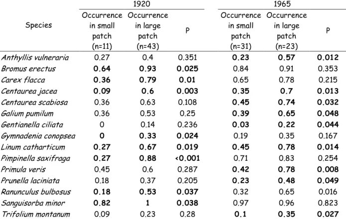
Contribution to extinction debt was measured using the 54 patches from all cartographic data. Of the 46 specialist species, 44 were present in at least one of the patches. Following our approach, 15 species contributing to extinction debt were identified (related to at least one historical date) (Table 5). Eight and nine of the species exhibited a significantly higher current occurrence in patches larger than 4.061 ha, in 1920 and 1965, respectively. Two of the species (Centaurea jacea and Linum catharticum), showed a significantly higher current occurrence in patches larger than 4.061 ha at both periods. Four other species (i.e. Carlina vulgaris, Gentianella germanica, Centaurium erythrea, and Polygala comosa) also exhibited a strong association to historically large grasslands, although the probability this correlation was due to chance was greater than 0.05 (Appendix 1).
Table 5: List of specialist species significantly contributing to extinction debt (at least with reference to one historical period) and their occurrence (% presence) in patches that were larger or smaller than the currently largest patch (large patch and small patch, respectively) at two historical dates (1920, 1965). n is the number of patches. P is the P -value associated with the Fisher Exact Test (FET). FET tested for a difference in occurrence between historically large and small patches. Species contributed to extinction debt at P < 0.05. Species 1920 1965 Occurrence in small patch (n=11) Occurrence in large patch (n=43) P Occurrence in small patch (n=31) Occurrence in large patch (n=23) P Anthyllis vulneraria 0.27 0.4 0.351 0.23 0.57 0.012 Bromus erectus 0.64 0.93 0.025 0.84 0.91 0.353 Carex flacca 0.36 0.79 0.01 0.65 0.78 0.215 Centaurea jacea 0.09 0.6 0.003 0.35 0.7 0.013 Centaurea scabiosa 0.36 0.63 0.108 0.45 0.74 0.032 Galium pumilum 0.36 0.53 0.25 0.39 0.65 0.048 Gentianella ciliata 0 0.14 0.236 0.03 0.22 0.044 Gymnadenia conopsea 0 0.33 0.024 0.19 0.35 0.167 Linum catharticum 0.27 0.67 0.019 0.45 0.78 0.014 Pimpinella saxifraga 0.27 0.88 <0.001 0.71 0.83 0.254 Primula veris 0.45 0.6 0.287 0.42 0.78 0.008 Prunella laciniata 0.18 0.37 0.205 0.23 0.48 0.049 Ranunculus bulbosus 0.18 0.53 0.037 0.32 0.65 0.016 Sanguisorba minor 0.82 1 0.038 0.97 0.96 0.823 Trifolium montanum 0.09 0.23 0.28 0.1 0.35 0.027
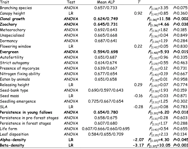
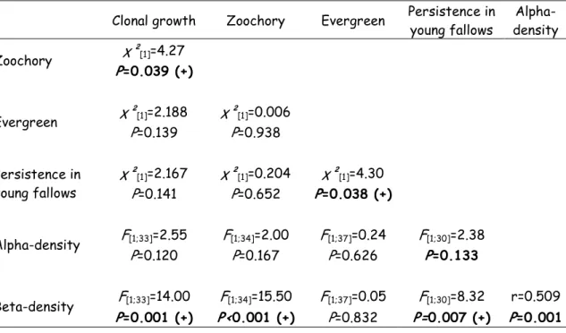
The magnitude of ALP (a measure of the association with historically large patches) was significantly associated with six of the 26 traits examined, including clonality, zoochory, evergreenness, high alpha and beta densities, and persistence in young fallow (Table 6). Species that exhibited at least one of the traits exhibited a lower association to historically large patches (lower ALP) than species lacking the traits. Therefore, they are likely to contribute less to extinction debt. Associations between these six traits are shown in Table 7. Evergreenness was indicated as one of the most independent traits, and was only correlated with persistence in young fallows (χ²[1]=4.30; P = 0.038). Beta-density was associated with all other traits, with the
exception of evergreenness.
Table 6: Relationships between traits and contribution to extinction debt (measured as the highest ALP - Association to historically Large Patches- detected for each species). Significant differences from mean ALP were tested with ANOVA for nominal and ordinal traits. Linear regressions (LR) between ALP and trait values were used for numeric traits. Mean ALP was estimated for each class of non-numeric traits (see Table 1 for order). T
represents the T-values for traits from linear regressions. Traits significantly associated to ALP are in bold.
Trait Test Mean ALP T
Branching species ANOVA 0.657/0.733 F[1;38]=3.35 P=0.075
Canopy height LR 0.92 F[1;42]=0.85 P=0.360
Clonal growth ANOVA 0.624/0.749 F[1;36]=11.58 P=0.002
Zoochory ANOVA 0.645/0.731 F[1;36]=4.66 P=0.038 Meteorochory ANOVA 0.692/0.643 F[1;36]=1.82 P=0.185 Unspecialised ANOVA 0.665/0.668 F[1;36]=0.04 P=0.849 Dormancy ANOVA 0.687/0.641 F[1;28]=1.19 P=0.284 Flowering window LR 0.22 F[1;42]=0.05 P=0.830 Evergreen ANOVA 0.594/0.698 F[1;42]=5.93 P=0.019 Autofertility ANOVA 0.651/0.687 F[1;32]=0.96 P=0.335
Strict autogamy ANOVA 0.614/0.674 F[1;29]=0.55 P=0.463
Presence of mycoryze ANOVA 0.639/0.667 F[1;31]=0.12 P=0.731
Nitrogen fixing ability ANOVA 0.677/0.654 F[1;40]=0.19 P=0.667
Eaten by animals ANOVA 0.651/0.658 F[1;18]<0.01 P=0.958
Releasing height LR 0.29 F[1;42]=0.07 P=0.774
Seed-bank type ANOVA 0.690/0.597/0.643 F[2;38]=1.93 P=0.159
Seed mass LR -0.16 F[1;32]=0.03 P=0.871
Seedling emergence ANOVA 0.725/0.667/0.654 F[2;31]=1.25 P=0.302
SLA LR -0.28 F[1;27]=0.08 P=0.783
Persistence in young fallows ANOVA 0.654/0.780 F[1;31]=6.20 P=0.018
Persistence in pre-forest stages ANOVA 0.658/0.675 F[1;31]=0.28 P=0.603
Persistence in forest stages ANOVA 0.607/0.680 F[1;31]=1.17 P=0.288
Life form ANOVA 0.607/0.666/0.660/0.695 F[3;40]=0.54 P=0.655
Leaf disposition ANOVA 0.584/0.655/0.709 F[2;35]=2.13 P=0.134 Alpha-density LR -2.07 F[1;37]=4.30 P=0.045
Table 7: Relationship between traits significantly associated to species contribution to extinction debt (measured with ALP). Relationship between two nominal traits, one nominal and one numeric trait, and two numeric traits was respectively tested by chi-square tests (χ²[degree of freedom]), ANOVA (F[degrees of freedom]), and regression (Pearson’s r[n=number of observations]).
P is the P-value for each test, significant values are in bold. (+) for chi-square tests indicates that the presence of one trait significantly promoted the presence of the other trait. (+) for ANOVA indicates that the presence of the nominal trait significantly increased the value of the numeric trait.
Clonal growth Zoochory Evergreen Persistence in young fallows Alpha-density Zoochory χ²[1]=4.27 P=0.039 (+) Evergreen χ²[1]=2.188 χ²[1]=0.006 P=0.139 P=0.938 Persistence in young fallows χ²[1]=2.167 χ²[1]=0.204 χ²[1]=4.30 P=0.141 P=0.652 P=0.038 (+) Alpha-density F[1;33]=2.55 F[1;34]=2.00 F[1;37]=0.24 F[1;30]=2.38 P=0.120 P=0.167 P=0.626 P=0.133 Beta-density F[1;33]=14.00 F[1;34]=15.50 F[1;37]=0.05 F[1;30]=8.32 r=0.509 P=0.001 (+) P<0.001 (+) P=0.832 P=0.007 (+) P=0.001
Discussion
Extinction debt in South-East Belgium calcareous grasslands
The probability that a plant community suffers from an extinction debt depends on the time since the habitat was altered, the extent of habitat fragmentation, and the nature of the alteration (Kuussaari et al. 2009). It is hypothesized that 1) an extinction debt is most likely to exist in landscapes where habitat fragmentation occurred recently, and 2) an extinction debt will be paid off faster in landscapes with large reductions in habitat (Hanski and Ovaskainen 2002; Kuussaari et al. 2009). Some support has been provided for the last hypothesis by extinction debt studies on semi-natural grasslands in Europe. In landscapes with <10% of the grasslands remaining, evidence of extinction debt has not been detected, compared to less fragmented grassland ecosystems (Adriaens et al. 2006; Cousins 2009; Cousins et al. 2007).
In contrast to these previous studies, our results point to an elevated extinction debt in a highly fragmented calcareous grassland landscape. The extinction debt was estimated at approximately 28% of the total species richness, and higher for specialist species (34 - 41% based on method and reference date). Cousins and Vanhoenacker (2010) demonstrated that extinction debt may differ with species specialization. We report a substantial decrease in calcareous grasslands, with an 87% loss in grassland area over c. 80 years, which is among the highest fragmentation levels in Europe for semi-natural grasslands (Krauss et al. 2010). Mean patch area and mean patch connectivity also strongly decreased within this time lag. This spatio-temporal dynamics was very similar to a neighboring landscape in the same region described by Adriaens et al. (2006), where an extinction debt was not reported for calcareous grasslands. One reason for differences between the two studies may be due to fragmentation timing. A sizable grassland reduction occurred during the last forty years in our study area; with an 83% decrease in area compared to 21% between 1920-1965. Provided such a recent fragmentation process, extinction debt may not be paid off, even in very small isolated remaining grasslands.
A second reason extinction debt estimations may differ among landscapes with similar history may be due to differences in methodology. If an empirical study fails to detect extinction debt, it is important to assess if adequate methods have been applied (Kuussaari et al. 2009). In this study, we employed two widespread methods that test for an extinction debt in communities of fragmented habitats (Kuussaari et al. 2009). Each method holds its own unique challenges. Therefore, it was relevant to our study that the approaches resulted in the same conclusions: calcareous grasslands suffered from an extinction debt. One difference was detected between the two approaches. The regression model did not indicate an extinction debt for 1920 total species, however a significant extinction debt (on average 26.51 species) was detected under the high loss/low loss model, which revealed the lowest probability (P = 0.032). Furthermore, the two methods showed a similar magnitude of extinction debt.
Results showed that current area exhibited the main effect on species richness. However, multiple regressions indicated that the variation in species richness that remained unexplained was in part due to patch history, suggesting a possible extinction debt in our study site. We concluded an extinction debt from the multiple regression approach primarily because we included area loss as an independent variable, in addition to past and current landscape structure. For a given present day area, grasslands that have lost a higher proportion of area in the last 40 years host a higher species richness, which can be interpreted as a legacy of their past spatial structure. If we excluded area loss in the regression models, an extinction debt would not have been detected for 1965, indicating a discrepancy among methods. This is an important point, because studies that have reported the absence of extinction debt (Adriaens et al. 2006; Cousins et al. 2007) in highly fragmented grasslands have done so based on the lack of a correlation with past landscape structure, and have not considered individual patch dynamics.
In our study, we had to eliminate numerous very small patches (< 0.048 ha) distributed in the current landscape, in order to make the current cartographic data comparable to the historic data. It is likely comparable grasslands were present in the past, but historical cartographic documents are not adequate to detect habitat details at this scale. Consequently, extinction debt could not be calculated in the very small patches using our present methodologies.
Species contribution to extinction debt
Identifying species that have not yet paid an extinction debt is important, as it may not be a random sample of the habitat species pool. The probability of an extinction debt likely depends on the life-history traits of a particular species. However, information is scarce on the influence of species traits on extinction debt (Kuussaari et al. 2009).
We developed a method that mirrors community extinction debt estimations to detect species where the present occurrence pattern in the landscape is influenced by past habitat configuration. Specifically, we tested whether the current specialist species occurrence in calcareous grassland patches was significantly associated to grasslands that have been historically larger than the current largest patch. This was the case for 15 specialist species. Among them, Trifolium montanum is critically endangered (CR), Gentianella ciliata is endangered (EN), and Gymnadenia conopsea is vulnerable (VU) at a regional scale following IUCN criteria (Saintenoy-Simon et al. 2006). In addition, in all cases where data were available, all specialist species were shown to have reduced fitness in small populations. Schleuning et al. (2009) showed that, in Trifolium montanum, isolation, population size and population density decreased seed production per individual. Gentianella ciliata exhibits a reduction in reproductive performance in small populations (Kéry and Matthies 2004), and limited populations of the species are more likely to go extinct than large populations. Primula veris exhibits lower fitness in small populations (Brys et al. 2003; Kéry et al. 2000). Centaurea jacea shows reduced germination rates as well as a lower seedling survival rate in small populations (Soons and Heil 2002).
It is worth noting that high ALP (= association with large patch) values were associated with several rare species for 1920, and species rarity rejected the hypothesis that distribution was due to chance. However, some common species (e.g. Bromus erectus and Sanguisorba minor) were significantly associated with former large patches, although their ALP values were close to 0.5, suggesting indifference (Appendix 1). The high number of observations for these common species may result in statistical significance, which does not always indicate ecological significance.
Our results suggested that species comprising scarce populations require larger habitat patches. It is likely these species cannot maintain relatively large populations in small habitat patches and contribute more to fragmentation. Species exhibiting persistence traits (clonality, evergreenness, persistence in young fallows, and density) were less dependent on large habitat patches. These traits were not independent; clonal species and species persistent in young fallows exhibited the highest beta-density. Clonal species are more likely to survive in small habitat patches and are often long-lived and less prone to extinction (Fischer and Stöcklin 1997; Poschlod et al. 2000). Other traits that reduce the risk of extinction, such as seed banks and long-term seed viability (Fréville et al. 2007; Stöcklin and Fischer 1999) might have similar effects, which were not observed in our study. This indicated that in our study landscape, species with transient seed banks are not more likely to support the extinction debt. Zoochory also appeared to reduce dependence on large habitat patches. In a large scale study, Römermann et al. (2008) demonstrated that epizoochorous species were underrepresented among declining species. However, because grazing was abandoned almost one century ago in our grasslands, an explanation for this effect is not clear. It is probably an artefact of the link between persistence and dispersal traits. We showed that clonal species are mainly zoochorous; this does not exclude an effect of dispersal ability itself. However, it is difficult to differentiate from clonality. We can therefore conclude that non-clonal, deciduous species that form sparse populations, that cannot persist in degraded habitats, are the most likely to pay an extinction debt. The present day occurrence of these species might be the heritage of a past landscape configuration.
Implications for conservation
Extinction debt had the greatest effect on remnant areas of fragmented habitat. However, we argue that the establishment of an extinction debt in a given habitat landscape can be considered a benefit. Most habitats respond slowly to fragmentation. Therefore, identifying an extinction debt enables managers to begin damaged habitat restoration with adequate time to implement recovery programs. The lag time inherent in an extinction debt is variable and difficult to predict. Vellend et al. (2006) argued that an extinction debt in forest habitat could persist for more than a century. A forest is hardly comparable to a grassland, but it is worth noting that Pärtel et al. (1998) and Zobel et al. (1996) estimated that 50-100 years are required to restore a calcareous grassland from a forest stand. However, response to restoration is species-dependent and many typical calcareous grassland species are able to rapidly colonize restored sites (Piqueray et al. 2011). Exclusive of the time necessary, restoration is required for the long-term conservation of fragmented habitats (Piqueray and Mahy 2010). Our study indicated that priority should be given to grassland patches that suffered a substantial loss in the past. It also showed that patches larger than the current maximum patch area are needed to maintain a set of specialist species that have not yet paid their extinction debt.
If extinction debt provides a new opportunity to support habitat restoration, it also imposes an undefined deadline. While we wait to launch large-scale restoration programs, the extinction debt payment is in progress.
Acknowledgements
This work was undertaken as part of the project “Development and test of a methodology for the elaboration of Natura 2000 sites designation acts”, funded by the Walloon Public Service (DGARNE-DNF). This study was supported by the FRS-FNRS (contract FRFC 2.4556.05).
R
EFERENCES
Adriaens D., Honnay O., Hermy M. (2006). No evidence of a plant extinction debt in highly fragmented calcareous grasslands in Belgium. Biol. Conserv. 133: 212-224.
Andrén H. (1994). Effects of habitat fragmentation on birds and mammals in landscapes with different proportions of suitable habitats: a review. Oikos 71: 355-366.
Balmford A., et al. (2005). The convention on biological diversity's 2010 target. Science 307: 212-213.
Berglund H., Jonsson B.G. (2005). Verifying an extinction debt among lichens and fungi in Northern Swedish boreal forests. Conserv. Biol. 19: 338-348.
Bisteau E., Mahy G. (2005). Vegetation and seed bank in a calcareous grassland restored from a Pinus forest. Appl. Veg. Sci. 8: 167-174.
Brys R., Jacquemyn H., Endels P., Hermy M., De Blust G. (2003). The relationship between reproductive success and demographic structure in remnant populations of Primula veris. Acta Oecologica 24: 247-253.
Butaye J., Honnay O., Adriaens D., Delescaille L.M., Hermy M. (2005). Phytosociology and phytogeography of the calcareous grasslands on Devonian limestone in Southwest Belgium. Belg. J. Bot. 138: 24-38.
Cousins S.A.O. (2009). Extinction debt in fragmented grasslands: paid or not? J. Veg. Sci. 20: 3-7.
Cousins S.A.O., Ohlson H., Eriksson O. (2007). Effects of historical and present fragmentation on plant species diversity in semi-natural grasslands in Swedish rural landscapes. Landscape Ecol. 22: 723-730.
Cristofoli S., Piqueray J., Dufrêne M., Bizoux J.P., Mahy G. (2010). Colonization credit in restored wet heathlands. Restor. Ecol. 18: 645-655.
Delescaille L.M. (1999). La gestion conservatoire des pelouses sèches par le pâturage ovin. Aspects théoriques et pratiques. Parcs & Réserves 54: 2-9.
Delescaille L.M. (2002). Nature conservation and pastoralism in Wallonia. Pages 39-52 in Redecker B., Finck P., Härdtle W., Riecken U., Schröder E., eds. Pasture landscapes and nature conservation. Berlin: Springer-Verlag.
Delescaille L.M. (2005). La gestion des pelouses sèches en Région wallonne. Biotechnol. Agron. Soc. Environ. 9: 119-124.
Draper N.R., Smith H. (1998). Applied regression analysis. New York: Wiley. 706 p.
Dupré C., Ehrlén J. (2002). Habitat configuration, species traits and plant distributions. J. Ecol.
90: 796-805.
Ellenberg H. (1974). Zeigerwerte von Pflanzen in Mitteleuropa. Scripta Geobotanica 9: 3-122. Ellis C.J., Coppins B.J. (2007). 19th century woodland structure controls stand-scale epiphyte
diversity in present-day Scotland. Divers. Distrib. 13: 84-91.
Fahrig L. (2003). Effects of habitat fragmentation on biodiversity. Ann. Rev. Ecol. Evol. Syst. 34: 487-515.
Fischer M., Stöcklin J. (1997). Local extinctions of plants in remnants of extensively used calcareous grasslands 1950-1985. Conserv. Biol. 11: 727-737.
Fréville H., McConway K., Dodd M., Sivertown J. (2007). Prediction of extinction in plants: interaction of extrinsic threats and life history traits. Ecology 88: 2662-2672.
Hanski I. (1994). A practical model of metapopulation dynamics. J. Anim. Ecol. 63: 151-162. Hanski I. (1998). Metapopulation Ecology. Oxford, UK: Oxford University Press. p.
Hanski I., Ovaskainen O. (2002). Extinction debt at extinction threshold. Conserv. Biol. 16: 666-673.
Helm A., Hanski I., Pärtel M. (2006). Slow response of plant species richness to habitat loss and fragmentation. Ecol. Lett. 9: 72-77.
Henle K., Davies K.F., Kleyer M., Margules C.R., Settele J. (2004). Predictors of species sensitivity to fragmentation. Biodiversity and Conservation 13: 207-251.
Jackel A.K., Dannemann A., Tackenberg O., Kleyer M., Poschlod P. (2006). Funktionelle Merkmale von Pflantzen und ihre Anwendungsmöglichkeiten im Arten-, Biotop- und Naturschutz.: Naturschutz und Biologische Vielfalt 32. 168 p.
Jackson S.T., Sax D.F. (2009). Balancing biodiversity in a changing environment: extinction debt, immigration credit and species turnover. Trends Ecol. Evol. 25: 153-159.
Karlík P., Poschlod P. (2009). History or abiotic filter: which is more important in determining the species composition of calcareous grasslands. Preslia 81: 321-340.
Kéry M., Matthies D. (2004). Reduced fecundity in small populations of the rare plant Gentianopsis ciliate (Gentianaceae). Plant Biology (Stuttgart) 6: 683-688.
Kéry M., Matthies D., Spillmann H.H. (2000). Reduced fecundity and offspring performance in small populations of thedeclining grassland plants Primula veris and Gentiana lutea. J. Ecol. 88: 17-30.
Kolb A., Diekmann M. (2005). Effects of Life-History Traits on Responses of Plant Species to Forest Fragmentation. Conserv. Biol. 19: 929-938.
Kuussaari M., et al. (2009). Extinction debt: a challenge for biodiversity conservation. Trends Ecol. Evol. 24: 564-571.
Lambinon J., Delvosalle L., Duvigneaud J. (2004). Nouvelle flore de Belgique, du Grand-Duché de Luxembourg, du Nord de la France et des régions voisines. Meise: Jardin botanique national de Belgique. p.
Leimu R., Mutikainen P., Koricheva J., Fischer M. (2006). How general are positive relationships between plant population size, fitness and genetic variation? J. Ecol. 94: 942-952.
Levins R. (1970). Extinction. Pages 77-107 in Desternhaber M., ed. Some Mathematical Problems in Biology. Providence: American Mathematical Society.
Lindborg R. (2007). Evaluating the distribution of plant life-history traits in relation to current and historical landscape configurations. J. Ecol. 95: 555-564.
Lindborg R., Eriksson O. (2004). Historical landscape connectivity affects present plant species diversity. Ecology 85: 1840-1845.
Mildén M., Cousins S.A.O., Eriksson O. (2007). The distribution of four grassland plant species in relation to landscape history in a Swedish rural area. Annales Botanici Fennici 44: 416-426.
Moilanen A., Nieminen M. (2002). Simple connectivity measures in spatial ecology. Ecology 83: 1131-1145.
Palm R. 2002. Macros Minitab pour la régression linéaire. (15th December 2008 2008;
http://www.fsagx.ac.be/si/reglin/accueil.htm)
Pärtel M., Kalamees R., Zobel M., Rosén E. (1998). Restoration of species-rich limestone grassland communities from overgrown land: the importance of propagule availability. Ecol. Eng. 10: 275-286.
Piessens K., Hermy M. (2006). Does the heathland flora in north-western Belgium show an extinction debt? Biol. Conserv. 132: 382-394.
Piqueray J., Bisteau E., Bottin G., Mahy G. (2007). Plant communities and species richness of the calcareous grasslands in southeast Belgium. Belg. J. Bot. 140: 157-173.
Poschlod P., WallisDeVries M.F. (2002). The historical and socioeconomic perspective of calcareous grasslands: lessons from the distant and recent past. Biol. Conserv. 104: 361-376.
Poschlod P., Kleyer M., Tackenberg O. (2000). Databases on life history traits as a tool for risk assessment in plant species. Zeitschrift für Ökologie und Naturschutz 9: 3-18.
Poschlod P., Karlík P., Baumann A., Wiedmann B. (2008). The history of dry calcareous grasslands near Kallmünz (Bavaria) reconstructed by the application of palaeoecological, historical and recent-ecological methods. Pages 130-143 in Szabó P., Hédl R., eds. Human nature: Studies in historical ecology and environmental history. Pruhonice: Institute of Botany of the Czech Academy.
Poschlod P., Kiefer S., Tränkle U., Fischer S., Bonn S. (1998). Plant species richness in calcareous grasslands as affected by dispersability in space and time. Appl. Veg. Sci. 1: 75-90. Poschlod P., Kleyer M., Jackel A.K., Dannemann A., Tackenberg O. (2003). BIOPOP - A database
of plant traits and internet application for nature conservation. Folia Geobot. 38: 263-271.
Prendergast J.R., Quinn R.M., Lawton J.H., Eversham B.C., Gibbons D.W. (1993). Rare species, the coincidence of diversity hotspots and conservation strategies. Nature 365: 335-337. Römermann C., Tackenberg O., Jackel A.K., Poschlod P. (2008). Eutrophication and fragmentation
are related to species' rate of decline but not to species rarity: results from a functional approach. Biodiversity and Conservation 17: 591-604.
Royer J.M. (1991). Synthèse eurosibérienne, phytosociologique et phytogéographique de la classe des Festuco-Brometea. Berlin-Stuttgart: J.Cramer. 296 p.
Saintenoy-Simon J., Barbier Y., Delescaille L.M., Dufrêne M., Gathoye J.L., Verté P. 2006. Première liste des espèces rares, menacées et protégées de la Région Wallonne (Ptéridophytes et Spermatophytes). (29th September 2008
http://mrw.wallonie.be/dgrne/sibw/especes/ecologie/plantes/listerouge/)
Schleuning M., Niggemann M., Becker U., Matthies D. (2009). Negative effects of habitat degradation and fragmentation on the declining grassland plant Trifolium montanum. Basic Appl. Ecol. 10: 61-69.
Schoenfeld D.A. 2007. Statistical considerations for clinical trials and scientific experiments. (2nd February 2009 http://hedwig.mgh.harvard.edu/sample_size/size.html)
Siegel S. (1956). Nonparametric statistics for the behavioral science. New York: McGraw Hill. 312 p.
Soons M.B., Heil G.W. (2002). Reduced colonization capacity in fragmented populations of wind-dipersed grassland forbs. J. Ecol. 90: 1033-1043.
Stöcklin J., Fischer M. (1999). Plants with longer-lived seeds have lower local extinction rates in grasslands remnants 1950-1985. Oecologia 120: 539-543.
Tilman D., May R.M., Lehman C.L., Nowak M.A. (1994). Habitat destruction and the extinction debt. Nature 371: 65-66.
Tremlová K., Münzbergová Z. (2007). Importance of species traits for species distribution in fragmented landscapes. Ecology 88: 965-977.
Vellend M., Verheyen K., Jacquemyn H., Kolb A., Van Calster H., Peterken G., Hermy M. (2006). Extinction debt of forest plants persits for more than a century following habitat fragmentation. Ecology 87: 542-548.
WallisDeVries M.F., Poschlod P., Willems J.H. (2002). Challenges for the conservation of calcareous grasslands in northwestern Europe: integrating the requirements of flora and fauna. Biol. Conserv. 104: 265-273.
Weiher E., van der Werf A., Thompson K., Roderick M., Garnier E., Eriksson O. (1999). Challenging theophrastus: a common core list of plant traits for functional ecology. J. Veg. Sci. 10: 609-620.
Zobel M., Suurkask M., Rosén E., Pärtel M. (1996). The dynamics of species richness in an experimentally restored calcareous grassland. J. Veg. Sci. 7: 203-210.
Appendix
Appendix 1: Specialist species with their occurrence in small and large patches, corresponding ALP (= association with large patches), Contribution, and Safeness.
1920 1965 Contribution Safeness Occurrence in small patch (n=11) Occurrence in large patch (n=43) ALP Occurrence in small patch (n=31) Occurrence in large patch (n=23) ALP Allium oleraceum 0.45 0.47 0.506 0.35 0.61 0.632 0.632 1 Anacamptis pyramidalis 0 0 - 0 0 - - - Anthyllis vulneraria 0.27 0.4 0.592 0.23 0.57 0.715 0.715 1 Brachypodium pinnatum 0.82 0.91 0.526 0.87 0.91 0.512 0.526 0.997 Bromus erectus 0.64 0.93 0.594 0.84 0.91 0.521 0.594 0.999 Carex caryophyllea 0.27 0.37 0.577 0.26 0.48 0.65 0.65 1 Carex flacca 0.36 0.79 0.685 0.65 0.78 0.548 0.685 1 Carex tomentosa 0.09 0.02 0.204 0.03 0.04 0.574 0.574 0.135 Carlina vulgaris 0 0.16 1 0.16 0.09 0.35 1 0.038 Centaurea jacea 0.09 0.6 0.869 0.35 0.7 0.662 0.869 0.999 Centaurea scabiosa 0.36 0.63 0.633 0.45 0.74 0.621 0.633 1 Centaurium erythrea 0 0.16 1 0.06 0.22 0.771 1 0.038 Cirsium acaule 0.09 0.21 0.697 0.1 0.3 0.759 0.759 0.998 Euphorbia cyparissias 0.91 0.91 0.499 0.9 0.91 0.503 0.503 0.382 Festuca lemanii 0.82 0.56 0.406 0.55 0.7 0.559 0.559 1 Galium pumilum 0.36 0.53 0.595 0.39 0.65 0.628 0.628 1 Gentianella ciliata 0 0.14 1 0.03 0.22 0.871 1 0.013 Gentianella germanica 0 0.16 1 0.1 0.17 0.642 1 0.038 Gymnadenia conopsea 0 0.33 1 0.19 0.35 0.642 1 0.792 Helianthemum nummularium 0.91 0.98 0.518 1 0.91 0.477 0.518 0.621 Himantoglossum hircinum 0 0.07 1 0.06 0.04 0.403 1 <0.001 Hippocrepis comosa 0.64 0.56 0.467 0.52 0.65 0.558 0.558 1 Koeleria macrantha 0.55 0.44 0.448 0.35 0.61 0.632 0.632 1 Koeleria pyramidata 0.09 0.02 0.204 0 0.09 1 1 0.135 Linum catharticum 0.27 0.67 0.712 0.45 0.78 0.634 0.712 1 Medicago lupulina 0.36 0.44 0.549 0.35 0.52 0.595 0.595 1 Neotinea ustulata 0 0.02 1 0 0.04 1 1 0.016 Onobrychis viciifolia 0.09 0.07 0.434 0.03 0.13 0.802 0.802 0.586 Ononis repens 0.27 0.53 0.662 0.39 0.61 0.611 0.662 0.999 Ophrys apifera 0 0.02 1 0.03 0 0 1 <0.001 Ophrys fuciflora 0 0 - 0 0 - Ophrys insectifera 0 0.09 1 0.06 0.09 0.574 1 <0.001 Orchis anthropophora 0 0.02 1 0 0.04 1 1 0.016 Orchis militaris 0 0.02 1 0.03 0 0 1 <0.001 Pimpinella saxifraga 0.27 0.88 0.764 0.71 0.83 0.538 0.764 1 Plantago media 0.36 0.58 0.615 0.45 0.65 0.591 0.615 1
Appendix 1 (continued) 1920 1965 Contribution Safeness Occurrence in small patch (n=11) Occurrence in large patch (n=43) ALP Occurrence in small patch (n=31) Occurrence in large patch (n=23) ALP Polygala comosa 0.09 0.35 0.793 0.23 0.39 0.634 0.793 0.925 Potentilla neumanniana 0.91 0.79 0.465 0.84 0.78 0.483 0.483 0.964 Primula veris 0.45 0.6 0.571 0.42 0.78 0.651 0.651 1 Prunella laciniata 0.18 0.37 0.672 0.23 0.48 0.679 0.679 1 Ranunculus bulbosus 0.18 0.53 0.746 0.32 0.65 0.669 0.746 0.999 Salvia pratensis 0.09 0 0 0.03 0 0 0 0.016 Sanguisorba minor 0.82 1 0.55 0.97 0.96 0.497 0.55 0.621 Scabiosa columbaria 0.55 0.6 0.526 0.48 0.74 0.604 0.604 1 Thymus praecox 0 0.02 1 0.03 0 0 1 <0.001 Trifolium montanum 0.09 0.23 0.719 0.1 0.35 0.782 0.782 0.999