HAL Id: hal-01360043
https://hal.archives-ouvertes.fr/hal-01360043
Submitted on 5 Sep 2016HAL is a multi-disciplinary open access
archive for the deposit and dissemination of sci-entific research documents, whether they are pub-lished or not. The documents may come from teaching and research institutions in France or abroad, or from public or private research centers.
L’archive ouverte pluridisciplinaire HAL, est destinée au dépôt et à la diffusion de documents scientifiques de niveau recherche, publiés ou non, émanant des établissements d’enseignement et de recherche français ou étrangers, des laboratoires publics ou privés.
Secure aggregation in wireless sensor networks
Wassim Drira, Chakib Bekara, Maryline Laurent
To cite this version:
Wassim Drira, Chakib Bekara, Maryline Laurent. Secure aggregation in wireless sensor networks. [Research Report] Dépt. Logiciels-Réseaux (Institut Mines-Télécom-Télécom SudParis); Services ré-partis, Architectures, MOdélisation, Validation, Administration des Réseaux (Institut Mines-Télécom-Télécom SudParis-CNRS). 2009, pp.58. �hal-01360043�
Secure Aggregation in Wireless Sensor
Networks
LOgiciels-R´eseaux Wassim Drira 09008-LOR
Chakib Bekara 2009
Secure Aggregation in Wireless Sensor Networks —oOo—
Abstract
The Wireless Sensor Networks (WSNs) are composed of a huge number of sensor nodes. The large number of nodes may lead to a huge amount of data in the network, causing the network to degrade performance and shorten its lifetime. The data aggregation techniques may be a solution to remane the redundancy of data and thereby reduce the number of packets transmitted in the network. Nevertheless, the data aggrega-tion causes some security vulnerabilities: impersonaaggrega-tion, denying having received data, dropping packets deliberately, alteration of the sensored readings and aggregation re-sults... In this report, we compare the performances get by two secure aggregation solutions: the Secure Aggregation for Wireless Networks (Hu et al. protocol) and the Secure Aggregation Protocol for Cluster-Based Wireless Sensor Network (SAPC). The analysis shows that Hu et al. protocol gives better performance than SAPC in terms of number of exchanged messages but it is vulnerable to simple attacks. This report describes both protocols and their performances and propose a new protocol based on binary trees and delayed aggregation result checking to improve the performance of SAPC.
Key-words: Security, wireless sensor network, aggregation, TinyOS, authentication.
R´esum´e
Les r´eseaux de capteurs sans fil sont compos´es d’un grand nombre de capteurs avec de faibles ressources en ´energie, en m´emoire et en calcul. Dans le but d’´etendre la dur´ee de vie de ces r´eseaux, l’agr´egation des messages s’av`ere comme une bonne solution pour diminuer le nombre de messages ´echang´es dans le r´eseau en ´eliminant les donn´ees redondantes et par suite l’´energie utilis´ee par les nœuds pour la communication. Mais cette solution peut avoir des cons´equences n´efastes sur la s´ecurit´e du r´eseau: l’int´egrit´e des messages, l’authentification, la pr´ecision des mesures. . . Dans ce rapport, nous comparons les performances obtenus par deux protocoles d’agr´egation s´ecuris´es: Secure Aggregation for Wireless Networks (le protocole de Hu et al.) et le protocole Secure Aggregation Protocol for Cluster-Based Wireless Sensor Network (SAPC). L’analyse montre que le protocole de Hu et al. donne de bons r´esultats en terme de nombre de messages, mais il est vuln´erable `a certaines attaques simples. Ce rapport d´ecrit les deux protocoles avec une analyse de leur performances et propose, en vue d’am´eliorer les performances de SAPC, un nouveau protocole d’agr´egation bas´e sur les arbres binaires et la v´erification retard´e du r´esultat d’agr´egation.
Mots-cl´es : S´ecurit´e, r´eseau de capteurs sans fil, agr´egation, TinyOS, authentification. —oOo—
Wassim Drira Chakib Bekara Maryline Laurent-Maknavicius Stagiaire Doctorant Professeur
TELECOM & Management SudParis - D´epartement LOR - CNRS 9 rue Charles Fourier 91011 Evry cedex
{Wassim.Drira|Chakib.Bekara|Maryline.Maknavicius}@it-sudParis.eu
Contents
Introduction 7
1 Wireless sensor networks and security issues 8
1.1 Introduction . . . 8
1.2 Operating Systems . . . 9
1.2.1 TinyOS . . . 9
1.2.2 Contiki . . . 13
1.3 Sensor security problems . . . 13
1.3.1 Very limited resources . . . 13
1.3.2 Unreliable Communication . . . 14
1.3.3 Unattended Operation . . . 14
1.4 Security Goals and Challenges . . . 15
1.5 Attacks on the wireless sensor networks . . . 16
1.6 Conclusion . . . 18
2 Secure data aggregation approaches in Wireless Sensor Networks 19 2.1 Introduction . . . 19
2.2 Secure Aggregation for Wireless Networks . . . 19
2.3 SHIA . . . 22
2.3.1 Query dissemination . . . 22
2.3.2 Aggregation commit phase . . . 22
2.3.2.1 Naive approach . . . 23
2.3.2.2 Improved approach . . . 23
2.3.3 Result-checking phase . . . 25
2.3.3.1 Dissemination of final commitment values . . . 25
2.3.3.2 Dissemination of off-path values . . . 25
2.3.3.3 Verification of inclusion . . . 25
2.3.3.4 Collection of confirmations . . . 25
2.3.3.5 Verification of confirmations . . . 26
2.4 SAPC . . . 26
2.5 A trust based framework for Secure data Aggregation in Wireless Sensor Network . . . 28
2.5.1 System model . . . 28
2.5.2 Threat model . . . 28
2.5.3 Josang’s Belief Model . . . 29
2.5.4 A trust based framework against false data injection . . . 29
3 Implementation and Tests 32 3.1 Introduction . . . 32 3.2 Implementation . . . 32 3.3 Tests . . . 33 3.3.1 SAPC . . . 33 3.3.2 Hu et al. . . 35 3.4 Conclusion . . . 35
4 SeBTIA: Secure binary tree in-network aggregation 37 4.1 Introduction . . . 37
4.2 Commitment tree . . . 37
4.2.1 Notations . . . 37
4.2.2 Ordered tree . . . 38
4.2.3 Formation of the commitment tree (binary tree) . . . 39
4.2.4 Logical representation of the commitment tree . . . 39
4.3 Protocol description . . . 41
4.3.1 Query Dissemination . . . 41
4.3.2 Cryptographic Security . . . 41
4.3.3 Aggregation-Commitment phase . . . 41
4.3.4 Result-checking Phase . . . 45
4.3.5 Elimination of malicious or faulty nodes . . . 46
4.4 Congestion complexity . . . 46
4.5 Implementation and tests . . . 49
4.6 Conclusion . . . 49
Conclusions & perspectives 50
Bibliography 51
Glossary 54
List of Figures
1.1 Health care motes . . . 9
1.2 Evolution of motes . . . 10
1.3 Logo TinyOS . . . 11
2.1 Forwarding packets with and without data aggregation . . . 20
2.2 Data aggregation illustration . . . 21
2.3 Aggregation and naive commitment tree in network context . . . 23
2.4 Process of node A (from Figure 2.3) deriving its commitment forest from the commitment forests received from its children . . . 24
2.5 Dissemination of off-path values: t sends the label of u1 to u2 and vice-versa; each node then forwards it to all the vertices in their subtrees . . . . 25
2.6 Cluster-based wireless sensor network . . . 26
2.7 Abstract architecture of the framework . . . 29
3.1 Number of messages sent by CH . . . 33
3.2 Minimum and maximum number of messages in the network . . . 33
3.3 Calculation time in a normal node . . . 34
3.4 Calculation time in CH . . . 34
3.5 Calculation cost comparison for CH vs simple node . . . 35
4.1 Encoding n-ary trees as binary . . . 39
4.2 Formation of the commitment tree . . . 40
4.3 Logical representation of the commitment tree . . . 40
4.4 An ordered aggregation tree of a network . . . 41
4.5 The aggregate-commit algorithm . . . 44
4.6 Needed labels by node 15 to build the commitment tree . . . 45
4.7 Exploration of tree branches . . . 47
4.8 Comparison of SHIA and SeBTIA messages complexity . . . 48
4.9 Execution time needed to prepare L1 . . . 49
A.1 Component diagram of the SAPC application . . . 56
A.2 Component diagram of the Hu et al. application . . . 57
List of Tables
1.1 The impact of 29-BYTES payload cipher on CPU consumption . . . 14 1.2 The impact of calculating 29-BYTE packet MAC on CPU consumption . . 14 1.3 Sensor network layers and denial-of-service defenses . . . 17 3.1 Memory space occupation in SAPC and Hu et al. protocols . . . 32 4.1 An example of the Aggregation-commitment phase execution in the
net-work shown in figure 4 (“X: Y” signifies that the instruction Y is executed in node X) . . . 43 4.2 Memory space occupation in SeBTIA . . . 49
Introduction
Nowadays, we are overwhelmed with a large number of data. Extracting relevant data and eliminating redundant data is an important concern for researchers. Those techniques are needed in wireless sensor networks, which contain a huge number of sensor nodes, each one generating some sensory readings toward the base station. The data aggregation extends the longevity of the wireless sensor networks as exchange messages are targeted, but it makes the network more vulnerable. Many secure data aggregation protocols have appeared in the literature. Our contribution is to implement and compare two protocols for the secure data aggregation: The Secure Aggregation Protocol for Cluster-Based wireless Sensor network (SAPC) [1] and Hu et al. protocol [2]. Then we propose a solution to improve the SAPC performances.
This report is organized as follows: chapter 1 first introduces the wireless sensor networks and the security threats. Chapter 2 gives the most important solutions for the data aggregation in wireless sensor networks, and then some comparative experimental results between SAPC and Hu et al. protocol. In chapter 4, we present a new aggregation framework based on the binary trees to extend SAPC and improve its performances. Finally we conclude this report with future research directions.
1
Wireless sensor networks and
security issues
1.1
Introduction
The Wireless Sensor Network (WSN) is a term used to refer to a wide network composed by a huge number of heterogeneous sensors deployed randomly and that communicate through some wireless technologies. Generally, there is a special node called a base sta-tion (BS) in the network that receives the data from the sensors, and forwards them to the network operator. Most of the time, the network topology can not be predicted, and is deployed in hostile or friendly environments. The development of microelectronics and wireless communication technologies are leading to produce tinier and low cost sensors although they still have limited energy, memory and computational resources. Wireless Sensor Networks are widely used in various applications. The most important ones are:
Military: WSNs can be used to supervise the country frontier and enemy movement during a war. As such various sensors can be placed in the network, to detect movement of persons or vehicles, to detect sounds and to get some geographical coordinates. They can be coupled with a camera to take photos and videos when needed. For example, at the frontier between the United States and Mexico, a WSN coupled with cameras, is deployed to detect person’s illegal penetration.
Environment: A WSN can be deployed to supervise air pollution, to detect forest fire, and also to detect submarine earthquake to prevent disasters like Tsunamis. It can be also deployed, for example, near a chemical factory to detect any emission of poisonous substances in the air or in a lake.
Buildings: A WSN can be deployed in a building or a factory to manage automatically air conditioning, electric lights. In addition, it is used in dams in Thailand to detect the vibrations and pressure.
Health care: The application can detect and analyze patients health from bio sensors which can collect pulse, temperature and blood pressure of the patient (figure 1.1).
With this application, the doctors can remotely monitor, diagnose and prescribe the patient when an emergency occurs [3].
Supply Chain: WSN can be used to monitor the cold chain, as studied in the project CAPTEURS [4, 5] to which TELECOM SudParis participates in designing a secure solution to supervise the goods temperature along the transportation.
Figure 1.1: Health care motes [6]
A sensor node or a mote is a component mainly composed by a micro-controller, a chip for the wireless communication and one or more sensors to measure the physical quantities (temperature, humidity, light, motion, vibration,...). There are various types of motes in the market, but the most used ones in research are mica, mica2 and tmote. Figure 1.2 shows a comparison between different motes and the evolution of their capacities and resources.
1.2
Operating Systems
There are two main operating systems used in wireless sensor networks: TinyOS and Contiki. We discuss in this section the characteristics of each of them.
1.2.1
TinyOS
TinyOS is an open source operating system for wireless sensor networks, featuring a component-oriented architecture. In addition, it minimizes the code size as required by
the severe memory constraints inherent to the sensor networks. TinyOS provides to de-velopers different libraries like the network protocols, distributed services, sensor drivers, and data acquisition tools – all of which can be used as-is or be further refined for a cus-tom application. TinyOS’s event-driven execution model enables the fine-grained power management yet allows the scheduling flexibility made necessary by the unpredictable nature of the wireless communication and physical world interfaces [8].
Figure 1.3: Logo TinyOS
The development of TinyOS began in 1999 in Berkley university. The newest version is TinyOS 2.1 launched in 2008. The system is developed in nesC, a C-like language. Currently, the maintenance and development of the operating system is assured by an international consortium, the TinyOS alliance.
The principal characteristics of the operating system are:
Event-driven: TinyOS is an event-driven operating system. A complete system config-uration is formed by ’wiring’ together a set of components for a target platform and application domain. Components are restricted objects with well-defined interfaces, internal state, and internal concurrency. Primitive components encapsulate hard-ware elements, e.g., radio, ADC, timer, or bus. Their interface reflects the hardhard-ware operations and interruptions [9].
Components and Bidirectional Interfaces: A component has a set of bidirectional command/ event interfaces implemented either directly or by wiring a collection of subcomponents. The compiler optimizes the entire hierarchical graph, validates that the program is free of race conditions and deadlocks [9].
Split-phase operations: are a typical use of bidirectional interfaces. A higher-level component issues a command to initiate activity in a hardware or software com-ponent. The command returns immediately, indicating the status of the request, even though the operation takes some time to complete. When done, the operat-ing component signals an event to the components that will take further action. Meanwhile, the processor may service other tasks and events, or sleep if no tasks are pending. Thus, interleaved execution and power management is provided sys-tematically throughout the entire set of TinyOS components [9].
Hardware Abstraction Architecture: The most important advantages of TinyOS is its compatibility with multiple platforms, at least nine platforms. It is also not that complicated to add or modify the platforms. TinyOS 2.0 uses a three-tier Hardware Abstraction Architecture that combines the strengths of the component model with an effective organization in the form of three different levels of abstraction. The top level of abstraction fosters portability by providing a platform-independent hard-ware interface, the middle layer promotes efficiency through rich hardhard-ware-specific interfaces and the lowest layer structures access to hardware registers and inter-rupts [10].
Scheduler: Two types of blocks compose the programs in TinyOS: tasks and event han-dlers. Tasks are not preemptive but an event preempts the task execution. The semantics of the tasks in TinyOS 2.x are different than those in 1.x. In 1.x, the task queue has a limited length and can include the same task multiple times. In 2.x, each task has its reserved place in the queue so it can have one or none in-stance there. The scheduler executes the tasks one by one until the queue becomes empty [11].
Timers: TinyOS 2.x offers a rich timer system. Three fundamental properties of timers are precision, width and accuracy. Three precision skills are defined : TMilli (1024 ticks per second), T32khz (32768 ticks per second) and TMicro (1048576 ticks per second). The width for the timer interfaces is 32-bits. The accuracy reflects how closely a component conforms to the precision it claims to provide. Accuracy is affected by issues such as clock drift and hardware limitations.
TinyOS defines five types of timer interfaces like Counter, LocalTime and Alarm [12].
Communication: TinyOS 2.1 does not support the TCP/IP stack but the next version will do. The majority of the platforms uses the norm 802.15.4 to define both physical and media access layers. Different network protocols are available like the collection, dissemination and Tymo (adapted version of DYMO).
Power Management: Energy is a critical concern in wireless sensor networks and hence it is a concern for TinyOS. The node goes on a sleep mode when no task is executed; also the TinyOS lets developers to active/disable the radio communication’s chip or to use the low power listening. In addition, TinyOS generates a small binary code so it needs low power to memorize it in RAM [13].
nesC language: nesC is an extension to C designed to embody the structuring concepts and execution model of TinyOS [14]. nesC adds support to components, envents handling and tasks to the C language.
TOSSIM: TinyOS simulator. TOSSIM allows to compile TinyOS applications into a simulation framework, where developers can perform reproducible tests and debug their code with the standard development tools.
1.2.2
Contiki
Contiki [15] is a small, open source, highly portable, multitasking computer operating system developed for use on a number of memory-constrained networked systems ranging from 8-bit computers to embedded systems on micro-controllers, including sensor network motes. Contiki provides multitasking and a built-in TCP/IP stack, it implements also a µIPv6 stack [16].
Contiki supports dynamic loading of programs and multi-threading programming [17]. It comes with a graphical simulator COOJA [18].
1.3
Sensor security problems
The WSNs are different from the computer networks as many constraints make the adap-tation of existing security solutions more difficult. So, it is important to understand those constraints to design more efficient security mechanisms [19]:
1.3.1
Very limited resources
The integration of the security mechanisms into the applications generates a memory overhead, computational overhead and more larger packets. This overhead should consider those two constraints:
Limited Memory and Storage Space: As depicted in figure 1.2, the sensor nodes have limited program memory, RAM, and non volatile storage space. So it is neces-sary to limit the code size of the security algorithm. For example Telos motes [20] have 60 KB as program memory, 2 KB as RAM memory and 128 KB for non volatile storage.
Power limitation: The energy is a scarce resource for a sensor node since the battery is almost not easily replaced or recharged. Therefore, the battery charge taken with the sensor node to the field must be kept to extend its life time and as a result the entire sensor network longevity. When implementing a cryptographic function or protocol within a sensor node, the energy impact of the added security code must be considered. For example, RC5 (Table 1.1) presented better performance in terms of CPU elapsed time (1.50 ms) while using only 11,059.2 CPU cycles and consuming 36.00 micro-joules to cipher a payload. It (Table 1.2) consumes 49.92 µJ to authenticate 29-BYTE packet.
Algorithm Time (ms) CPU cycles Energy (µJ) SkipJack 2.16 15,925.2 51.84 RC5 1.50 11,059.2 36.00 RC6 10.78 79,478.7 258.72 TEA 2.56 18,874.4 61.44 DES 608.00 4,482,662,4 14,592.00
Table 1.1: The impact of 29-BYTES payload cipher on CPU consumption [21]
Algorithm Time (ms) CPU cycles Energy (µJ) SkipJack 2.99 22,044.6 71.76
RC5 2.08 15,335.4 49.92
RC6 15.84 116,785.2 380.16 TEA 5.07 37,380.1 121.68 DES 1,208.00 8,906,342.4 28,992.00
Table 1.2: The impact of calculating 29-BYTE packet MAC on CPU consumption [21]
1.3.2
Unreliable Communication
The sensor network uses wireless communications so it inherits the unreliability of the communications. This technology is characterized by sharing the same media, air, which has a high error rate and a concurrent access, consequently some frequent collisions hap-pen. In addition, the multi-hop nature of the network makes the synchronization between the nodes difficult due to the time needed in each hop to treat the message and forward it. This may be a problem for some security protocols that use a cryptographic key distribution protocol like µtesla [22].
1.3.3
Unattended Operation
Depending on the application of the sensor network, sensor nodes may be left unattended for a long period of time. There are three main caveats to unattended sensor nodes:
Exposure to Physical Attacks The sensor may be deployed in an environment open to adversaries, may be affected by bad weather, and so on. The likelihood that a sensor suffers from a physical attack in such an environment is therefore much higher than the typical PCs, which are located in a secure place and mainly face attacks from the network [19].
Remote Management Remote management of a sensor network makes it virtually im-possible to detect physical tampering (i.e., through tamperproof seals) and physical maintenance issues (e.g., battery replacement). Perhaps the most extreme example of this is a sensor node used for the remote reconnaissance missions behind the
en-emy lines. In such a case, the node may not have any physical contact with friendly forces after deployment [19].
No Central Management Point A sensor network is like a distributed network with-out a central management point. If designed incorrectly, it will make the network organization difficult, inefficient, and weak.
Passive information gathering An intruder can eavesdrop the exchanged messages in the network by positioning malicious nodes or a powerful receiver in the network.
False Node An intruder can maliciously disrupt the network operations for example by injecting a false node so their he is able to drop the packets, inject false data, or modify the contents of a message and hence corrupt the integrity of the message [23].
Node Malfunction A node may become defective for ordinary reasons and, therefore, output wrong data. This can be more dangerous if the node is an aggregator or a cluster head.
Node outage In addition to malfunctioning, a sensor may stop responding completely, for example if its battery is empty.
1.4
Security Goals and Challenges
In order to defend against some attacks, many security mechanisms have been proposed. The goal of each one is to achieve some or all of the following security goals [24]:
Confidentiality or privacy Confidentiality means that only the authorized parties can access the data. For example the confidentiality is a big concern in some cases like military applications or when exchanging the security keys between nodes.
Integrity It means that the transmitted data have not been altered during transit by unauthorized parties.
Authentication It means that the received data are really sent by the claimed sender instead of being injected by someone else.
Availability It means that the network should consistently and continually provide the service that it promises despite the existence of any attacks [23].
Freshness It means that the data are fresh and current. It guarantees that the messages are not replayed or injected by any adversary.
1.5
Attacks on the wireless sensor networks
The attacks, their classes and their classification by the layer are further discussed in [25]. The most important attacks in WSN are:
1. Passive information gathering see 1.3.3.
2. Node subversion By compromising a node, an attacker can get the program, the secret cryptographic keys thereby it becomes possible to inject false messages from this node. [26] demonstrates that compromising a Mica2 ’s node is done in one minute. For some applications, it becomes necessary to design the tamper resistant nodes. For example, a node should delete its program memory content and its secret keys once the node capture occurs.
3. Fake node see 1.3.3.
4. Node malfunction see 1.3.3.
5. Node outage see 1.3.3.
6. Message corruption The integrity of a message is compromised when an attacker modifies its content.
7. Traffic analysis Even if the message is encrypted in WSN, an attacker can anal-yse the communication patterns and detect which nodes are important in the net-work (e.g. cluster heads, aggregators,...) and focus on them to cause more harm to the network.
8. Routing loops An attacker can alter and replay routing information messages, thus some error messages are generated in the network. The routing loops attract or repel the network traffic and increase the node to node latency.
9. Selective forwarding If all the nodes participate in routing messages, an attacker can drop certain messages instead of forwarding them all. The percentage of dropped messages and the distance from the malicious node to the base station determine the effectiveness of this attack.
10. Sinkhole attacks The attacker places a malicious node in a key point (close to the base station). The node drops all the received messages instead of forwarding them to the base station. The result of this attack is more disrupting if there is a unique BS in the network.
11. Sybil attacks In this attack, a node declares multiple illegitimate identities either by forging or stealing the identities of legitimate nodes. This attack can be used against routing algorithms, topology maintenance and voting scheme.
Network layer Attacks Defenses
Physical Jamming Spread-spectrum, priority messages, lower duty cycle, region mapping, mode change Tampering Tamper-proofing, hiding
Link
Collision Error-correcting code Exhaustion Rate limitation Unfairness Small frames Network
and Routing
Neglect and greed Redundancy, probing Homing Encryption
Misdirection Egress filtering, authorization, monitoring Black holes Authorization, monitoring, redundancy Transport Flooding Client puzzles
Desynchronization Authentication
Table 1.3: Sensor network layers and denial-of-service defenses
12. Node replication The attack is made by adding a node, with a replicated (copied) ID of an existing node, to the targeted sensor network. The attacker can copy also cryptographic keys in the malicious node. This attack can result in a disconnected network, false readings
13. Wormhole An attacker records the packets at one location in the network, tun-nels them (possibly selectively) to another location, and retransmits them into the network. This attack can form a serious threat against the routing protocols and the location-based wireless security systems [27].
14. Hello flood attack The malicious node broadcasts a HELLO message with a strong transmission power and pretends that it is coming from the base station. The receiving nodes assume that the malicious node is the closest one to the BS, so they send their data through it. In this attack, the responding nodes to HELLO floods waste their energy.
15. DoS attacks DoS appears as any event that diminishes or eliminates a network capacity to perform its expected function (Hardware failures, software bugs, resource exhaustion, environmental conditions, or their combination; or intentional attack). This attack targets the availability (which ensures that the authorized parties can access data, services, or other computer and network resources when requested) by preventing the communication between the network devices or by preventing a single device from sending the traffic [28].
1.6
Conclusion
WSNs become widely used in many applications and the security becomes a key concern to those networks. The traditional security approaches in wirelined and wireless networks are not merely applicable to WSN due to the resource limitation of the nodes and obstacles encountered by those networks.
This report focuses on data aggregation. In the next chapter, we discuss the interest for aggregation technique as well as we list some security protocols supporting the data aggregation.
2
Secure data aggregation
approaches in Wireless Sensor
Networks
2.1
Introduction
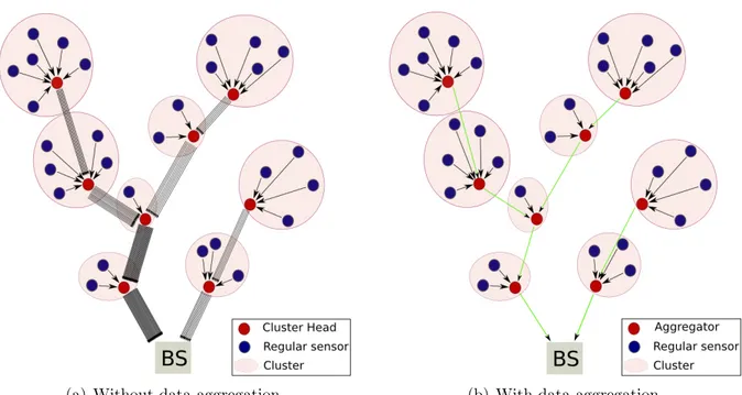
WSNs are composed by a huge number of sensor nodes. Figure 2.1(a) shows an important number of messages exchanged inside a network in response to a query sent by the BS. The large number of nodes may lead to a huge amount of data in the network, causing the network to degrade its performance and shorten its lifetime. The data aggregation techniques may be a solution to remove the redundancy of data and thereby reduce the number of packets transmitted in the network. For those reasons, some nodes can have the responsibility of aggregating data (messages) before transmitting them to BS. Figure 2.1(b) shows a network where the cluster heads (CH) have the data aggregation capability. We remark that the number of messages is significantly decreased when using the aggregator nodes in the network. Nevertheless, the data aggregation causes some security vulnerabilities: impersonation, denying having received data, dropping packets deliberately, alteration of sensory readings and aggregation results,...
Many security solutions have been proposed in the literature to secure the aggregation process, the most important ones are depicted in this chapter.
2.2
Secure Aggregation for Wireless Networks
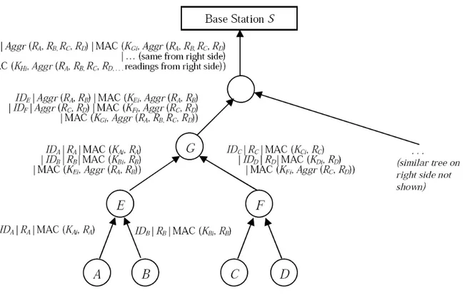
In [2], Hu et al. present a secure aggregation protocol for the wireless sensor networks, it is the first article that handles this problem. In this protocol we consider the existence of one powerful node called a base station (BS) which can broadcast messages to all the nodes directly. The other nodes are all identical and organized in a binary aggregation tree rooted by the BS. Some are acting as leaves (nodes A-D in Figure 2.2) and they are responsible for the sensing activities, and the others are acting as intermediate nodes. The aggregation is done only in intermediate nodes and BS. The protocol evolves in two steps:
(a) Without data aggregation. (b) With data aggregation.
Figure 2.1: Forwarding packets with and without data aggregation
delayed aggregation and delayed authentication. Exchanged messages are authenticated with temporary keys. The temporary key is computed by encrypting a counter value using a key shared between the node and the BS. For example KAS is the key shared
between the node A and the BS, and KA0 = E(KAS, 0) is a temporary key of A. After
the aggregation phase, the BS reveals the temporary keys to enable other sensor nodes to authenticate messages transmitted by nearby sensors. The counter is incremented after each cycle. The processing of aggregation is done as follows (see the network presented in Figure 2.2):
1. Each leaf node N transmits a message to its parent containing its unique identifier and its sensory reading; the message is authenticated by a secret key KN i only
known at that moment N and BS. For example :
A → E : RA|IDA|M AC(KAi, RA)
2. Upon receiving the messages from its children, the parent node cannot verify their authenticity, so it has to store the messages and verify them later when receiving KN i. It waits until receiving all its children messages or the waiting timer expiration
and then it sends a message to its parent that retransmits that sensory readings and MACs, along with a computed MAC over the calculated aggregate value. For example :
E → G : RA|IDA|M AC(KAi, RA)
Figure 2.2: Data aggregation illustration
|M AC(KEi, Aggr(RA, RB))
Note that E does not send IDE to G since G knows enough about the network
topology.
3. Upon receiving the messages from E and F, node G calculates the aggregation result of its grandchildren sensory readings through each child. It then associates the ag-gregation result of its grandchildren and its children’s ID and MAC values in a mes-sage; along with a MAC that it computes with its secret key KGi over the next
ag-gregate result, Aggr(RA, RB, RC, RD) = Aggr(Aggr(RA, RB), Aggr(RC, RD)),and
it sends the message to its parent. For example the message sent from G to its parent is:
IDE|Aggr(RA, RB)|M AC(KEi, Aggr(RA, RB))
|IDF|Aggr(RC, RD)|M AC(KF i, Aggr(RC, RD))
|M AC(KGi, Aggr(RA, RB, RC, RD))
4. The processing described in (3) is recursively repeated upstream until reaching the BS. So, in our case, node H receives the messages from its children, and sends the aggregate message to the BS.
5. Upon receiving the messages from its children, the BS calculates the final aggre-gation result. Then it broadcasts the authentication keys used by all the nodes in this aggregation round to let them verify the authenticity of the already received messages. Then the nodes verify the MACs and trigger an alarm if it does not match.
This protocol guarantees the authenticity of the messages for the networks where two consecutive nodes are not compromised. So, the compromising of two nodes as closest as possible to the BS, makes the attacker more powerful to falsify the final aggregation result.
We had implemented and tested this protocol, the results of this work are discussed in 3.3.2.
2.3
SHIA
Secure hierarchical in-network aggregation in sensor networks (SHIA) [29] is a secure SUM aggregation protocol. This protocol is useful for sum, count, average and median calculations. It has three main phases : query dissemination, aggregation commit and result checking.
2.3.1
Query dissemination
The base station broadcasts a query to the network. An aggregation tree is established if it is not already present. The query message contains a nonce value N to prevent replay of messages and it is authenticated.
2.3.2
Aggregation commit phase
Sensory data and aggregation results are included in a data structure called label. Label’s format is < count, value, complement, commitment > where count is the number of leaf vertices in the subtree rooted at this vertex; value is the SUM aggregate computed over all the leaves in the subtree; complement is the aggregate over the COMPLEMENT of the data values; and commitment is a cryptographic commitment. The labels are defined inductively as follows: There is one leaf vertex us for each sensor node s, which we call
the leaf vertex of s. The label of us consists of count = 1, value = as where as is
the sensory value of s, complement = r − as where r is the upper bound on allowable
data values, and commitment is the node’s unique ID. Internal vertices represent the aggregation operations, and have labels that are defined based on their children. Suppose an internal vertex has child vertices with the following labels: u1, u2, · · · , uq, where
v =P vi and h = H[N ||c||v||v||u1||u2||...||uq]. Two approaches are described in this phase
the naive approach and the improved approach:
2.3.2.1 Naive approach
Leaf nodes in the aggregation tree (e.g. node G in the figure 2.3) send their leaf vertex to their parent. The internal node (like A in figure 2.3) aggregates all the received labels and its leaf vertex, and sends the resulted label to its parent.
Figure 2.3: Aggregation and naive commitment tree in network context
2.3.2.2 Improved approach
This approach aims to improve the congestion cost in forming balanced aggregation trees. The difference from the last approach is that nodes aggregate only labels with the same depth (count). The leaf sensor nodes in the aggregation tree originate a single label which they then communicate to their parent sensor nodes. Each internal sensor node s originates a similar single label. In addition, s also receives labels from each of its children. s receives one or more label from each of its direct children. It then combines all the labels (its single label and the received ones) to form a new set of labels as follows. Suppose s wishes to combine q labels L1, · · · , Lq. We let the intermediate result be
SL = L1 ∪ · · · ∪ Lq, and repeat the following until no two labels have the same count
in SL: Let c the smallest count such that more than one label in SL has count c. Find two labels Li and Lj of count c in SL and merge them into a label of count (2 × c) by
creating a new label that is the parent of both Li and Lj. When no two labels have the
same count in SL, node s sends the set of labels SL to its parent. This process in node A is described in figure 2.4.
Figure 2.4: Process of node A (from Figure 2.3) deriving its commitment forest from the commitment forests received from its children
2.3.3
Result-checking phase
This phase lets each sensor s verify that its sensory data as were added into the SUM
aggregate and the complement (r − as). Each sensor verifies that its label was included in
the calculation of the final root label. Thus by inspecting the inputs and the aggregation operations in the commitment tree. This phase is split into five steps:
2.3.3.1 Dissemination of final commitment values
After the BS has received the final set of labels, it sends each of these labels to the entire sensor network using an authenticated broadcast.
2.3.3.2 Dissemination of off-path values
To enable verification, each leaf vertex must receive all its off-path values. Each internal node sends any labels received from its parent to all its children. It sends also the set of labels received from its child u to all its other children (Figure 2.5).
Figure 2.5: Dissemination of off-path values: t sends the label of u1 to u2 and vice-versa;
each node then forwards it to all the vertices in their subtrees
2.3.3.3 Verification of inclusion
When the node us receives all the labels of its off-path vertices, it may then verify the
labels until obtaining the root set of labels and verify that the received from the BS and the calculated ones are equal.
2.3.3.4 Collection of confirmations
After the successful verification of inclusion, each sensor node s sends an acknowledgment to the BS with form M ACks(N ||OK) to the BS. Those messages are XOR-ed hop by hop.
2.3.3.5 Verification of confirmations
When the BS receives the XOR-ed acknowledgments, it calculates an XOR-ed acknowl-edgment and verifies that the received and the calculated ones are equal.
2.4
SAPC
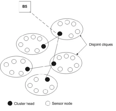
In the Secure Aggregation Protocol for Cluster-Based wireless Sensor network (SAPC) [1], nodes are organized into disjoint cliques (clusters), thanks to Sun et al. protocol [30], where each node is one-hop away from the remaining nodes of the cluster. Then nodes in each cluster elect a Cluster-Head (CH) from them to act as a CH and an aggregator, to communicate with the BS, and roots other CHs messages to BS. The organization of the network is described in figure 2.6. In addition, the nodes share a secret key with the BS, initially loaded before deployment. Also, each pair of nodes within the same clique shares a pairwise key to authenticate their messages. To authenticate its locally broadcast messages, each node u generates a one-way key chain {Kn
u}, and u sends the commitment
key of the key chain to each neighbor, authenticated with the pairwise key.
Figure 2.6: Cluster-based wireless sensor network
The aggregation is done in each cluster, and all the nodes participate in its calculation. The BS, which knows the list of sensors per cluster, can check whether the aggregation
result of a cluster was approved by cluster members or not. An aggregation round is described by four main steps, the lth aggregation round in the cluster C headed by node
CHi (CCHi) is done as follows :
1. Each node u in the cluster broadcasts its sensory reading Ru authenticated with the
current key Kj
u of its key chain
u → ∗ : RukM ACKj
u(Ru)kK
j u
2. Each node v ∈ CCHi receives all the broadcasted reading messages of u (∀u ∈
CCHi\{v}). For each received message, v verifies it by following those steps :
(a) verify the authenticity of the key Kj
u (Kuj−1 = H(Kuj)), if succeeded then
(b) verify the MAC field
If the two conditions are accepted, node v stores the key Kj
u (to use it to verify the
u’s reading message in the next round). Note that this key is used once, so it is never used to authenticate another message.
After receiving all the reading messages, the node calculates the aggregation result : AGRv = f (Ru/∀u ∈ CCHi).
Then node v prepares a double authenticated message, the first MAC is generated by the pairwise key KBS,v, shared between node v and BS, over the aggregation
AGRv and counter Cv where Cv is a counter shared between node v and BS and
it is used to protect BS from replay attacks. The second MAC is calculated over AGRv and the first MAC with the pairwise key shared between node v and CHi.
Node v sends this message to CHi:
v → CHi :
1
z }| {
AGRvkM ACKBS,v(AGRv, Cv) kM ACKCHi,v(1)
3. The CHi verifies all the received messages using the secret pairwise keys.
Unauthen-ticated messages are ignored. Logically all the messages contain the same aggrega-tion result, but it might exist some malicious or faulty nodes (less than the majority in the cluster), or some nodes which have not received all the reading messages due to collisions. Anyway, the cluster adopts the majority aggregation result AGR, it XORs the MACs for BS from the messages with the aggregation result equal to AGR, and finally it authenticates the message with its shared pairwise key with BS and sends it to BS. Node IDs with different aggregation results are included in the message.
CHi → BS : 2 z }| { AGRk M v∈CCHi M ACKBS,v(AGRv, Cv) kM ACKBS,CHi(2)
4. Upon receiving the message sent by CHi, the BS verifies its authenticity using
KBS,CHi. If authenticated, BS proceeds in the verification of the XOR-ed MAC
by calculating a set of MACs using the set of its shared keys with cluster nodes and then XOR them. If the calculated and received MACs are equal, the result is authenticated, otherwise it is rejected (Note that BS excludes the MACs of the nodes which sent a different aggregation result to CHi).
2.5
A trust based framework for Secure data
Aggre-gation in Wireless Sensor Network
2.5.1
System model
In this framework [31], we consider those assumptions:
• a static sensor network composed of a large number of densely deployed sensors which are organized into clusters
• in the network model, all the nodes are similar but they have three different behav-iors :
– sensor nodes send their sensory reading values to an aggregator
– aggregator collects readings, aggregates them and sends a report to CH – CH aggregates the received reports from the aggregators and forwards the
aggregated results to the BS (sink)
• in one cluster, all the sensor nodes including the CH and aggregators are physically close to each other and hence their sensory data are highly correlated
• every sensor node has a pairwise key with its one-hop neighbors, and uses it in a MAC for authentication.
2.5.2
Threat model
In this model, the attacker can inject/replay messages, compromise a sensor node either physically by capturing the node or by spreading a malicious code, and obtain all the secret materials.
2.5.3
Josang’s Belief Model
Josang’s model [31] proposes a belief metric to express an opinion about an aggregation result. It defines a quadruple w = (b, d, u, a) where b is belief, d is disbelief, u is un-certainty, a is relative atomicity; a, b, d, u ∈ [0, 1] and b + d + u = 1. The opinion O is calculated as
O = E(w) = b + au (2.1)
This model is suitable to capture the uncertainty in data aggregation in WSNs since the sensory data and aggregation results are infiltrated with uncertainties due to the unavoidable sampling errors, false data injected by either compromised source nodes or aggregators.
2.5.4
A trust based framework against false data injection
The aggregation process in the protocol is as follows:
Figure 2.7: Abstract architecture of the framework [31]
• Each sensor node reports its sensory data to its corresponding aggregator. The sensory data should be protected by a MAC with the pairwise key shared between the node and its aggregator.
• Upon receiving reports from sensor nodes, the aggregator does those steps :
– It eliminates sample values significantly deviated from the median
– The sensing data of the sensor nodes follow a normal distribution : N (µ, σ), where µ is the mean and σ is the standard deviation. In a long run, if the sampling is independent between each round, the probability of one node’s
sensory data falling in [µ − σ, µ + σ] should be 0.68, this is ideal node frequency (fideal) distribution. Some aggregators calculate the parameters µ and σ, then
they update each actual node frequency (fa).
– The aggregator calculates the Kullback-Leiber (KL) distance between the ideal and actual distributions for each node. The KL distance D is calculated as follows : D = (1 − fa)log2( 1 − fa 1 − fideal ) + falog2( fa fideal )
– Aggregator calculates the reputation of each sensor node as 1 1 +√D
– Aggregator dynamically classifies sensor nodes, according to their reputation, into K groups with the K-Means partition algorithm.
– After classifying the nodes, the aggregator calculates the average (x) of sensory values of nodes in the highest reputation group as well as the standard deviation (σ) as its aggregation result in this round.
– The aggregator counts the number of nodes having their sensory values within [x − σ, x + σ] and treats those nodes as trustworthy for this aggregation round. – The aggregator A formulates its opinion wA
X = {bA, dA, uA, aA} about the
ag-gregation result X as follows:
∗ bA: percentage of nodes fall in [x − σ, x + σ]
∗ uA= 1 − bA
∗ aA: average reputation of the uncertain nodes
∗ dA= 0
∗ the expectation of the aggregator’s opinion about aggregation result X is OXA = bA+ aAuA
– The aggregator sends its report, composed by aggregation result and opinion, to the cluster head.
• Upon receiving reports from aggregators, cluster head compares its own sensing data with the received aggregation results. It formulates an opinion about aggregators on two steps:
– It opts for the majority value and considers nodes with this value as honest and treats the rest as dishonest.
– The number of times the aggregator A is considered as honest by the cluster head (H) is noted by kH
A; and lHA is the contrary. The cluster head opinion
about aggregator A, wH A = (bHA, dHA, uHA, aHA) is obtained by: bHA = k H A kH A + lHA + 2 , dHA = l H A kH A + lHA + 2 , uHA = 2 kH A + lHA + 2
OH
A like defined in equation (2.1).
• This step is known as belief discounting, in which the cluster head formulates an opinion about each aggregator report X. This by discounting of wXA (the aggre-gator A opinion about its aggregation result X which is included in its emitted report) by wH
A (opinion of cluster head H about aggregator A) to obtain wXHA =
(bHA X , dHAX , uHAX , aHAX ) where bHAX = bHA × bA X, dHAX = bHA × dAX, uHAX = dHA + uAH + bAH × uA X, aHAX = aAX.
The expectation of the cluster head’s opinion about the aggregator’s report is OHA
X =
bHAX + aHA × uHA X .
• Finally, as the cluster head receives a report from each aggregator, suppose that they are two aggregators, the final aggregation result is calculated by X = ω1X1+ ω2X2,
where ω1 and ω2 are weighting factors defined as
ω1 = OHA1 X OHA1 X + O HA2 X , ω2 = OHA2 X OHA1 X + O HA2 X
The cluster heads send its report to the base station.
In addition to its role of sensing and reporting data to its aggregator, the sensor node overhears the transmitted reports by aggregators and cluster head to update their reputations. The cluster members can reselect an aggregator or cluster head either if their reputation drops below a certain threshold or to balance energy consumption between nodes by rotating periodically the roles.
2.6
Conclusion
In this chapter, we show different approaches to secure data aggregation in WSNs. In the next chapter we compare two protocols SAPC and Hu et al.
3
Implementation and Tests
3.1
Introduction
Many secure aggregation protocols are proposed in the litterature, as described in the pre-vious chapter. It exists two types of protocols: some protocols perform local aggregation in the clusters [1, 31] and the others perform hop-by-hop data aggreagtion [2, 29]. We selected two protocols from the two different types for implementing and testing which are SAPC [1], the protocol proposed by our laboratory, and Hu et al. [2] protocol. The evaluation of the performance is based on two criteria: the message complexity and the computation time. The message complexity is defined as a measure where the overhead of the protocol is measured in terms of number of messages needed to satisfy the protocol’s request [32]. The computation time is measured on a tmote sky [33] sensor node which uses a 16-bit, 8MHz Texas Instruments MSP430 microcontroller with only 10 KB RAM, 48KB Program space, 1024 KB External flash, and which is powered by two AA batteries. Results of this work are the concern of this chapter.
3.2
Implementation
We implemented SAPC and Hu et al. protocols in TinyOS 2.x to test and analyze them. The memory spaces occupied in a tmote sky sensor by a node (not a BS) program are described in the table 3.1. In this implementation, we use CBC-MAC RC5 to authenticate the messages as it requires minimum CPU cycles and execution time [21].
Memory space SAPC Hu et al. ROM (bytes) 29124 26364 RAM (bytes) 3308 3215
3.3
Tests
3.3.1
SAPC
Let’s start with the analysis of the number of messages sent in the SAPC protocol. The node in the cluster should send at least two messages in each round of the aggregation and the CH should broadcast one message containing its reading and another to the BS containing the aggregation result, but the CH should also forward the aggregation messages of other CHs to the BS. So in the optimized case, a CH sends two messages when it is a leaf in the routing tree or when all CHs are one hop away from the BS. The figure 3.1 compares the maximum and minimum numbers of messages sent or forwarded by a CH. For example in a network of 400 nodes, the maximum number of messages is 37. If we calculate the total number of messages in the network by adding the number of messages sent or forwarded by each node in one round, the maximum number is 1430 messages and the minimum is 800 (Figure 3.2).
Figure 3.1: Number of messages sent by CH
Figure 3.2: Minimum and maximum number of messages in the network
Now let us evaluate the calculation time needed by a simple node (neither CH nor BS) to accomplish its tasks (figure 3.3), i.e. to:
• receive other reading messages, verify the authentication key (Kj
u = H(Kuj−1)) and
then verify the MAC
• calculate the aggregation result and authenticate this message with two MACs
For this node, it takes 146.4 ms to accomplish those tasks in a cluster formed of 11 nodes. The distribution of this time between different tasks is described in figure 3.3. The CH, in addition to the previous tasks has to receive the aggregation messages, verify them and calculate the final aggregation result. The final aggregation result compu-tation includes XORing the MACs of all the nodes having the same result, authenticating the message and finally sending it to the BS. To accomplish those tasks in a cluster formed of 11 nodes, it takes a total calculation time of 187,5 ms in a CH. The distribution of this time between different tasks is described in figure 3.4.
Figure 3.5 compares the calculation cost for a CH vs a simple node, according to the total number of nodes in the network. Note that the two calculation costs are close although a simple node implements fewer functions than a CH. We can deduce that the position of the node in the hierarchy has little impact on the calculation cost.
Figure 3.3: Calculation time in a normal node
Figure 3.5: Calculation cost comparison for CH vs simple node
3.3.2
Hu et al.
In this protocol we can differentiate between three kinds of nodes: (1) leaf nodes, (2) aggregator nodes with leaf nodes descendants and (3) aggregator nodes with aggregators descendants.
The leaf node generates a message containing its reading (sensored data) and sends it to its parent. The aggregator of types (2) or (3) receives two messages from its descendants and then it sends a message to its parent. In fact, each node in this protocol sends one message but the aggregators should receive two others; this is independent of the number of nodes in the network and if we suppose that our network is organized into a binary tree.
In our implementation, each node uses its authentication key once and sends it with the message. The authenticity of the key is verified before the verification of the authenticity of the message.
A node of type (1) needs 4,0283 ms to prepare the message containing the sensored data and to perform the authentication. Nodes of type (2) need 19,683 ms to verify the authenticity of the keys and received messages, to calculate the aggregation result and to authenticate it. Nodes of type (3) need 44,616 ms to verify the authenticity of the three keys and the three MACs in each received message, to calculate the aggregation result and authenticate it.
3.4
Conclusion
We remark that in the Hu et al protocol, the number of messages is constant, and equal to the number of nodes in the network. Each node sends a unique message whatever its type. In SAPC, the number of messages depends on the number of nodes, the position and role of the node. So, it is constant for a simple node and equal to 2; but it is variable for the CH; it is in the range of 2 to 11 in a 40 node network and in the range of 2 to 37 in a 400 node network. The length of the data messages used in the implementation is
52 bytes in Hu et al, and 30 bytes in SAPC.
The verification of the reading messages consumes most of the time in SAPC. It takes 90% of the total execution time in a simple node and 70% in the CH. An attack with replayed or forged reading messages might cause an important calculation overhead in the sensor node. The security of the Hu et al. aggregation result can be altered if there are two consecutive malicious nodes not being detected.
In the next chapter, we present a new aggregation protocol to enhance the perfor-mances of SAPC by aggregating the exchanged messages. In addition to the local cluster aggregation, we propose a solution to do the hop by hop aggregation based on the binary distributed commitment tree.
4
SeBTIA: Secure binary tree
in-network aggregation
4.1
Introduction
A node in a wireless sensor network sends its measurements to a BS and it can route the messages of other nodes. If it has not direct communication with the BS, it sends them to an intermediate node. So the network is organized like a tree: BS is the root, and the sensor node is a leaf if it does not route other nodes messages otherwise it is an intermediate node. Each node knows its direct children and its parent which is BS or an intermediate node. A distributed algorithm can be used to build this tree like the described one in [34]. The BS knows the organization of the tree, and each rearrangement should be authorized by the BS. We call this tree an aggregation tree.
The hop-by-hop data aggregation is an interesting way to reduce the communication overhead and energy expenditure of the sensor nodes. Although, the data aggregation can let malicious or faulty nodes deviate the result, we propose in this chapter a protocol that lets the sensor nodes and the BS verifying the final aggregation result to eliminate the malicious nodes. The protocol has two phases: an aggregation-commitment phase to collect sensory data and aggregate them hop-by-hop, and a verification phase in which the sensor nodes verify that their sensory data have been included in the aggregation result. If there is a negative acknowledgment, the BS eliminates the suspected malicious nodes.
4.2
Commitment tree
4.2.1
Notations
• BS : Base Station
• Ot: Ordered aggregation tree
• Bt: commitment tree or binary tree
• D(Ot, A, i): the child number i of A in Ot(children are numerated from left to right)
• P (Ot, A): A’s parent in Ot
• LA
i : label i of node A. Its form is organized in < N, A, i, nA, vA, commitment >
– N : a value to guarantee the freshness of the messages, it can be a nonce value included in the query disseminated by the BS or a counter incremented in each round of aggregation. It is a unique value used by all the nodes during the aggregation round.
– A: the node’s identifier – i: a value in the range [0..2]
– nA: the number of nodes in the subtree rooted by A
– vA: the aggregation result of the subtree
– commitment: cryptographic value. This field is noted next as hA
• f: is the aggregation function (max, min, mean, . . . ) with two parameters as inputs for function like max or min or with four parameters as inputs for functions like mean (f (vB, vA, nB, nA) =
vB× nB+ vA× nA
nB+ nA
)
• H: the hash function used to calculate the commitment value
• F : L × L → L LA
i+1 = F (LBj, LAi )
=< N, A, i + 1, nB+ nA, f (vB, vA), H(N, A, i + 1, nB+ nA, f (vB, vA), hB, hA) >
where L is the set of all possible labels
• KA−B: a pair wise key used to authenticate messages between nodes A and B
• KA: a pair wise key used to authenticate the messages between node A and the BS
4.2.2
Ordered tree
The obvious method that a vertex can use to order its children is based on their identifier. In our protocol, we are going to use three parameters. First, the vertex orders them decreasingly based on their number of descendants. This order is not total; the vertex can have some children with equal number of descendants. Second, it can rearrange them increasingly based on the depth of the subtree rooted by those nodes. This order is not total too; finally children with equal numbers of descendants and depth are ordered based on their unique identifier.
When each node in the aggregation tree orders its children, we obtain an ordered aggregation tree.
4.2.3
Formation of the commitment tree (binary tree)
There is a one-to-one mapping between the general ordered trees and binary trees, which in particular is used by Lisp to represent general ordered trees as binary trees [35]. Each node N in the ordered tree corresponds to a node N0 in the binary tree; the left child of N0 is the node corresponding to the first child of N, and the right child of N0 is the node corresponding to N’s next sibling (the next node in order among the children of the parent of N). For example figure 4.1, in the left tree, A has the 6 children B,C,D,E,F,G. It can be converted into the binary tree on the right.
Figure 4.1: Encoding n-ary trees as binary
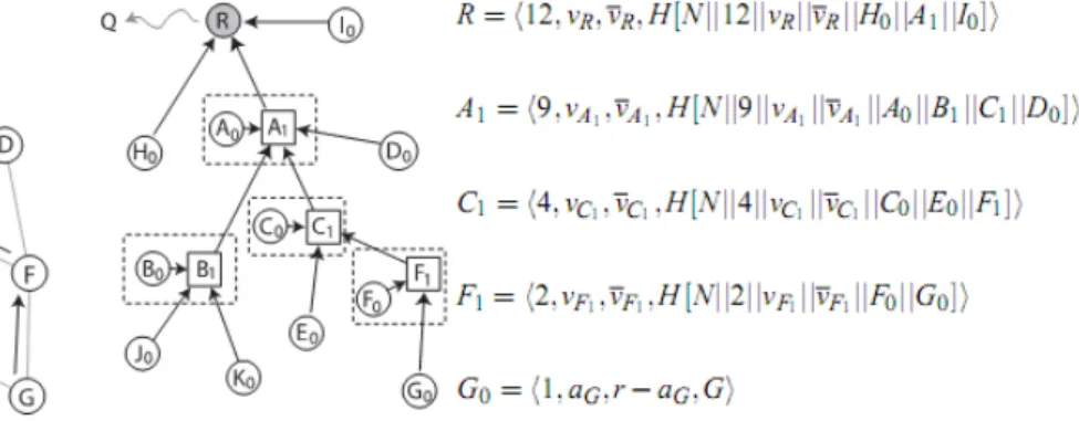
We apply this algorithm on an ordered aggregation tree as defined in paragraph 4.2.2 to form a commitment tree. This formation is distributed in each intermediate node, which knows only its children, and is able to organize them and send the result to its parent. So the real structure of the tree is not known by any node, only the BS knows the organization of nodes and then of the commitment tree. An example of a commitment tree is the right tree in figure 4.2, the left tree is an ordered (routing) tree. Before describing the commitment tree formation process in section 4.3, we describe how to represent the tree nodes and labels in a graph.
4.2.4
Logical representation of the commitment tree
In the commitment tree, a node can at most have three links. Each link means a label calculation. The logical representation of the commitment tree is represented in figure 4.3.
• ID: Identifier of the node, for example the identifier of the highlighted node in bold is 23
• L23
Figure 4.2: Formation of the commitment tree
• L23
1 : Label 1 of node 23 is the result of function F applied on L382 and L230 . L231 =
F (L382 , L230 ). The node sends Label 1 to its parent. If a node has no child in the routing tree, its Label 1 will be equal to its Label 0.
• L23
2 : Label 2 of node 23 is the result of function F applied on L152 and L231 . This
Label is calculated by the parent of node 23 in the routing tree. If a node has not a right child in the commitment tree (e.g. has not a right sibling in the ordered routing tree), its Label 2 is equal to its Label 1.
Note that all the labels of a leaf node (in the commitment tree) are equal.
4.3
Protocol description
4.3.1
Query Dissemination
Our protocol may be used first to aggregate the nodes responses to a query disseminated by the BS. This query can be authenticated by using an authentication protocol like µ-tesla [22] or H2BSAP [36]. Second, if nodes should periodically send a report contain-ing their measurements of some physical phenomenon to the BS, those reports can be aggregated thanks to our protocol.
4.3.2
Cryptographic Security
Exchanged messages between nodes are authenticated by a pairwise key. When a node receives a message, it verifies that N0 used in the label is equal to N used in the current aggregation round. Then it verifies the number of descendants (each node knows the number of descendant of its children). Finally it verifies the message authentication code with the corresponding pairwise key.
4.3.3
Aggregation-Commitment phase
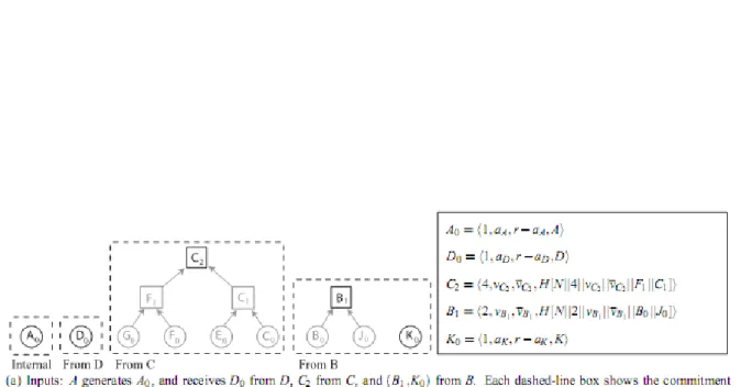
The algorithm of this phase is described in figure 4.5. In the beginning, each node prepares its initial label L0.
Figure 4.4: An ordered aggregation tree of a network
If node M has no child in the routing tree, its labels L1 and L0 are equal. M sends L1
to its parent.
If M has one or more child, it waits until receiving all its children labels or until the expiration of a waiting timer. If timer expires before receiving all labels, identifiers of
nodes missing labels are included in the message routed to the BS; this parent and its children are marked by BS.
Based on the ordered aggregation tree defined in paragraph 4.2.2; the last M’s child on the right has not right child in the binary tree, so its label L2 is equal to its label L1.
If M has more than one child, it calculates label L2 of next children one by one from the
left to the right until calculating L2 of the first child on the left. After the calculation of
label L2 of the M’s first child on left, or if M has only one child: M calculates its label
LM
1 and sends it to its parent if it has a parent otherwise it is the root (BS).
An execution sample of this algorithm in the network presented in figure 4.4 is illus-trated in Table 4.1. 19: L19 1 = L190 19 → 15 : L19 1 , M ACK19−15(L 19 1 ) 15: L192 = L191 15: L151 = F (L152 , L150 ) 26: L26 1 = L026 5: L51 = L50 15 → 7 : L15 1 , M ACK7−15(L 15 1 ) 26 → 7 : L261 , M ACK7−26(L 26 1 ) 5 → 20 : L5 1, M ACK20−5(L 5 1)
7: L262 = L261 7: L152 = F (L262 , L151 ) 7: L7 1 = F (L152 , L70) 20: L5 2 = L51 20: L201 = F (L52, L200 ) 2: L2 1 = L20 7 → 1 : L71, M ACK7−1(L 7 1) 20 → 1 : L20 1 , M ACK20−1(L 20 1 ) 2 → 1 : L21, M ACK2−1(L 2 1) 1: L22 = L21 1: L202 = F (L22, L201 ) 1: L72 = F (L202 , L71) 1: L1 1 = F (L72, L10) 1: L1 2 = L11 ⇒ L1
2 is the final label of the aggregation
Table 4.1: An example of the Aggregation-commitment phase execution in the network shown in figure 4 (“X: Y” signifies that the instruction Y is executed in node X)
4.3.4
Result-checking Phase
The BS broadcasts securely the final label in the network using a secure broadcast pro-tocol.
To let each node verify that its label has been included in the aggregation process, it needs some labels to build the aggregation tree until obtaining the root label and verifying that the received and calculated labels are equal. For example in the aggregation tree, figure 4.6, the root label is L1
2. The node 15 needs some labels, which are highlighted on
green, to build the commitment tree.
Figure 4.6: Needed labels by node 15 to build the commitment tree
So, each internal node A in the aggregation tree should send some information to its children:
• All labels that A receives from its parent
• its label 0 (LA 0)
• If A has more than one child, it sends to its first child B on the left in Ot, the label
2 of B’s next sibling in Ot
• To its child B, the Labels 1 of all B’s left siblings and Label 2 of B’s next sibling if B is not the last.
When the node receives all the necessary data to build the commitment tree, it verifies that its label has been included in the aggregation process by verifying that the received and the calculated final labels are equal.
Then each node sends an authentication code to the BS:
• otherwise M ACKs(N kN o); let us refer to as N O − ACK
Ok and N o are unique message identifiers; and Ks is a pairwise key shared between
the BS and node s. To minimize the amount of data sent to the BS, each node XOR its authentication code with its children and sends the result to its parent.
The BS verifies the consistency of the aggregation result by calculating
M ACK1(N ||Ok)XOR · · · XOR M ACKn(N ||Ok)
and then it verifies that the calculated and the received values are equal.
4.3.5
Elimination of malicious or faulty nodes
In this protocol we proceed differently from the method proposed in [37]. In the latter case, they use two adversary localizer schemes to mark and eliminate misbehaved nodes. In result-checking phase, they use an XORed MAC for each level in the commitment tree and in the second scheme they use big encrypted messages. The major weakness of this protocol is big messages which are very dependent on the network size and architecture. In our protocol we proceed by branch in the aggregation tree so we explore branches where there is a ACK. By exploring the branch, we can find the node N that has NO-ACK so we mark it and its parent M. If M is not already marked, it becomes a leaf. Its descendants (S : the set of M’s descendants) become roots of their subtree. An algorithm to rearrange the tree is triggered. The BS requests nodes in S to seek for a new parent; a HELLO message is sent by each node in S and add responding nodes to the list of its possible parents (nodes in S should not respond to the HELLO message). Then each node sends its list to the BS; the BS reorganizes the tree by choosing the new parent of the nodes in S. Different and not marked parents are the most preferred.
Nodes marked twice and those which do not send the potential parent list are elimi-nated from the network. The children of elimielimi-nated nodes are added to S.
For example in figure 4.7, A is the BS. A receives XORed MAC from all its children, it verifies it and it finds that in E’s branch there is a NO-ACK. So the BS demands from E its Ack and the XORed MACs of its children. E has an OK-ACK, so BS asks the E’s children to send ACKs and the XORed MACs of their children. A discover that K has a NO-ACK so it marks E and K. E becomes a leaf, K and L seeks for a new parent that is preferably not already marked.
4.4
Congestion complexity
In the aggregation commitment phase, each node sends one label to its parent for whatever the number of its children. In the result-checking phase, each node needs some off-path
Figure 4.7: Exploration of tree branches
labels to generate the aggregation tree and obtain the final label. Let’s define the depth of a node in the commitment tree by the minimum number of hops from it to the root plus one. So the root depth is one. Node 15 depth, in figure 4.6, is three. The number of labels needed by each node, except the root, is in the range [n-1, 2(n-1)], where n is the node depth.
Proof: The extreme number of messages in the range [n-1, 2(n-1)] are reached when the commitment tree is a full binary tree.
• Depth n=2: the tree is composed of one root and two child like figure 4.3.
– node 38 needs L23
0 and L152 : 2 × (2 − 1) = 2
– node 15 needs only L123: 2 − 1 = 1
• Suppose that a node in extreme left needs 2(n-1) labels and a node in extreme right needs (n-1) labels.
• Demonstrate it for nodes in depth n+1 (range [n,2n])
– As described in 4.3.4, a node A in extreme left with depth (n+1) has a parent B in extreme left too with depth n. B sends to A the labels that it has already received, LB
0 and label 2 of A sibling. So A receives 2 × (n − 1) + 2 = 2 × n
labels
– As described in 4.3.4, a node C in extreme right with depth (n+1) has a parent D in extreme right too with depth n. D sends to C the labels that it has already received, LD
![Figure 1.1: Health care motes [6]](https://thumb-eu.123doks.com/thumbv2/123doknet/11450483.290645/10.892.109.788.323.671/figure-health-care-motes.webp)
![Figure 1.2: Evolution of motes [7]](https://thumb-eu.123doks.com/thumbv2/123doknet/11450483.290645/11.892.108.788.383.893/figure-evolution-of-motes.webp)
![Table 1.2: The impact of calculating 29-BYTE packet MAC on CPU consumption [21]](https://thumb-eu.123doks.com/thumbv2/123doknet/11450483.290645/15.892.239.655.355.490/table-impact-calculating-byte-packet-mac-cpu-consumption.webp)