Order Number: ... Series: ...
Faculty of Exact Sciences and Sciences of Nature and Life Computer Science Department
THESIS
In Candidacy for the Degree of
DOCTOR 3
rdCYCLE IN COMPUTER SCIENCE
Option: Artificial IntelligenceBy
S
OUMIAM
ANCERTITLE
A CPN-Approach for Distributed
Abductive Reasoning
Application to Causal Model-Based Diagnosis
Defended on: 29/06/2020 in front of the jury composed of:
Mr. Laid Kahloul Professor at the University of Biskra President Mr. Hammadi Bennoui Professor at the University of Biskra Supervisor Mr. Allaoua Chaoui Professor at the University of Constantine 2 Examiner Mr. Mustapha Bourahla Professor at the University of M’sila Examiner Mr. Abdelhamid Djeffal Associate Professor at the University of Biskra Examiner
T
his thesis deals with fault diagnosis of distributed systems from a model-based view where Coloured Petri Nets are used to describe the system behaviour. The systems concerned here are those comprising different interacting subsystems. Coloured Behavioural Petri Nets are defined as a particular CPN intended for the description of a system’s causal behaviour, where each transition is labelled with a matrix describing explicitly its firing ways. The use of such matrices helps in tackling the problem of complexity during backward analysis, and gives rise to a very specific technique based on reachability of CBPNs called CW-analysis. CBPNs together with the CW-analysis are used to develop a dis-tributed model-based diagnosis approach. The diagnostic system is defined as set of diagnostic agents where each is assigned to diagnose a subsystem. Accordingly, the system model consists of a set of place-bordered CBPNs, whereas CW-analysis is exploited to implement a local diagnosis scheme. Once local diagnoses are ob-tained by the different agents, a cooperation process should be initiated to ensure global consistency of such diagnoses.key-words: Model-based diagnosis, Causal models, Petri nets, Reachability analysis, CW-analysis.
C
ette thèse traite le problème du diagnostic des pannes dans les systèmes distribués à partir d’une approche basée-modèle où les réseaux de Petri colorés (CPNs) sont utilisés pour décrire le comportement du système. Les sys-tèmes concernés ici sont ceux comprenant différents sous-syssys-tèmes en interaction. Les réseaux de Petri colorés comportementaux (CBPNs) sont définis comme un CPN particulier destiné à la déscription du comportement causal d’un système, où chaque transition est étiquetée avec une matrice décrivant explicitement ses modes de franchissement. L’utilisation de telles matrices aide à résoudre le prob-lème de la complexité lors de l’analyse en arrière et donne lieu à une technique très spécifique basée sur l’accessibilité des CBPNs, appelée CW-analysis. Les CBPNs et la CW-analysis sont utilisés pour développer une approche de diag-nostic basée-modèle distribué. Le système de diagdiag-nostic est défini comme un ensemble d’agents où chacun est chargé de diagnostiquer le sous-système associé. En conséquence, le modèle du système consiste en un ensemble de CBPNs avec places de frontières, tandis que la CW-analysis est exploitée pour realiser le diag-nostic local. Une fois les diagdiag-nostics locaux obtenus par les différents agents, un processus de coopération doit être engagé pour assurer la cohérence globale de ces diagnostics.Mots-clés: Diagnostic basé-modèle, Modèles causaux, Réseaux de Petri, Anal-yse d’accessibilité, CW-analysis.
Firstly, and foremost, I would like to thank God for giving me the strength, knowledge, ability and opportunity to undertake this research study and to persevere and complete it satisfactorily.
I would like to take this opportunity to express my gratitude to my supervisor professor Hammadi Bennoui for the continuous support of my PhD study, for his patience and motivation. Thank you Sir for encouragement, advice, and support through ups and downs all those years.
I also thank those who agreed to be the referees of this thesis and allocated their valuable time in order to evaluate the quality of this work: Prof. Laid Kahloul, Prof. Allaoua Chaoui, Prof. Mustapha Bourahla and Dr. Abdelhamid Djeffal for their examination of the report and their valuable comments.
Special thank is dedicated to Prof. Kazar Okba, director of LINFI laboratory. Also, I express my very special appreciation to Mr. M’hamed Mancer (my brother), Mr. Abd Alhakim Cheriet and Mrs. Amira Mohammedi for the consistent support along my study years, and for the hand giving to me each time I get stacked.
My sincere thanks go to my best family ever, my parents, my brothers, and my sisters for their deep love and sincere support for me. Thank you so much.
Page
List of Figures vi
1 Introduction 1
I Preliminaries
8
2 Model-Based Diagnosis & Petri Nets 9
2.1 Introduction . . . 10
2.2 Principles of Model-Based Diagnosis . . . 12
2.2.1 Approaches to model-based diagnosis . . . 12
2.2.2 Unified framework for MBD . . . 15
2.2.3 Distributed Model-Based Diagnosis . . . 17
2.3 Petri Nets . . . 19 2.4 PN-Based Diagnosis . . . 25 2.4.1 Brief survey . . . 25 2.4.2 BPN-based diagnosis . . . 26 2.5 Discussion . . . 29 2.6 Conclusion . . . 31
II Contributions
33
3 Coloured Behavioural Petri Nets 34 3.1 Introduction . . . 353.2.1 Structure of CBPNs . . . 36 3.2.2 Dynamic Behaviour of a CBPN . . . 40 3.3 Example . . . 41 3.4 BPN-CBPN Translation . . . 43 3.4.1 Translation procedure . . . 43 3.4.2 Proof of correctness . . . 49 3.5 Conclusion . . . 51
4 CW-Analysis for Diagnostic Problem Solving 52 4.1 Introduction . . . 53
4.2 CW-analysis . . . 53
4.2.1 Formal definition . . . 54
4.2.2 Analysis algorithm . . . 57
4.3 Formalizing Diagnosis with CBPNs . . . 59
4.4 Diagnostic problem solving within CBPNs . . . 61
4.5 Conclusion . . . 63
5 Modular CBPN-Based Diagnosis 64 5.1 Introduction . . . 65
5.2 System model . . . 66
5.3 Local preliminary diagnosis . . . 67
5.4 Cooperation between agents . . . 72
5.5 Conclusion . . . 75
6 Conclusion 77
FIGURE Page
2.1 A presentation of diagnostic activity . . . 11
2.2 A diagnostic system architecture. . . 18
2.3 Petri net corresponding to a ∧ b → c . . . 21
2.4 CPN corresponding to Example. 2.1 . . . 24
2.5 Backward firing rules of a BPN. . . 28
3.1 Fork transition . . . 37
3.2 Possible cases of join transition . . . 38
3.3 FW-matrix decomposition . . . 38
3.4 CBPN corresponding to Example. 2.1 . . . 39
3.5 A CBPN example. . . 42
3.6 Reachability graph of CBPN of Fig. 3.5. . . 43
3.7 BPN examples representing a system’s different behaving modes. . . . 47
3.8 The CBPN corresponding to the BPNs of Fig. 3.7. . . 48
4.1 The CW-analysis graph of Example 3.3 . . . 57
5.1 A modular CBPN . . . 68
C
H A P1
I
NTRODUCTION
Ever since humans have been developing systems where an increasing number of them are dedicated, of course, for the facilities of daily life. For instance, there are many well-known examples in application areas such as medical devices, aircraft flight control, nuclear systems, household appliances, and so on. For such systems, high performance, product quality, and cost-efficiency are continuously required, besides the insistent demands for more system reliability, availability, security, and safety. Unfortunately, the fact is "any human-made system is prone to fail", system failures are relatively common. On average, these failures cause inconvenience but no serious, long-term damage. However, this would not be the case all the time, some failures result in loss of life, significant property damage, or damage to the environment. Concerning such undesirable effects, the need for effective means to deal with them is quite apparent. For this very issue, fault diagnosis has been extensively appreciated in both industry and academia.
Global Overview and Motivation
From a general perspective, fault diagnosis can be explained as follows. Any designed system has a behaviour, obviously defined in terms of its observed
variables, for which it is known a priori when it is normal (often called the expected behaviour). At some point in time, an observation over the system is made, e.g., checking the temperature degree. When the made observation does not coincide with what is expected, it indicates a symptom, and so a system failure (usually, a system failure is defined to be any deviation of the system from its normal behaviour). The task of fault diagnosis is to, given such a symptom, generate a diagnosis statement, thus to determine the causes leading the system to misbehave, which helps effectively to get the system back to well-functioning. Therefore, different branches of science have carried out the problem of fault diagnosis such as mechanical engineering, electronics, automatic control, and computer science. A great deal of research effort has been spent on the design and development of efficient diagnostic systems, which gives rise to a variety of approaches and schemes.
Model-based diagnosis (MBD) is a general approach, whose efficiency in deal-ing with system failures has been demonstrated by a great number of successful applications in different sectors. Here, the diagnosis is performed on the basis of a mathematical model of the system behaviour. The main idea consists in the comparison between the observed behaviour and the one which can be predicted using the system model. It has been adopted practically in two distinct and paral-lel research communities. The Fault Detection and Isolation (FDI) community has evolved in the automatic control field from the seventies and uses techniques from control theory and statistical analysis. The DX community emerged more recently, with foundations in the fields of computer science and artificial intelligence (AI).1
Generally, the diagnostic activity comprises two components: the system model and the diagnosis process itself (i.e., the search strategy). Along the line of AI, qualitative causal models with logic are used to describe the system behaviour, while the search for the cause of a system failure is abductive reasoning. For the sake of simplicity, the system model is qualitative because it uses a particular terminology such as "high/low temperature". In this case, the system variables (states) are characterized by a few discrete values. On the other hand, the model
1While the FDI approach focuses on fault detection in dynamical systems, the DX approach
focuses on diagnosis reasoning. A discussion of a common approach for methods used by the FDI and DX communities has been investigated not very early ([16], [17]).
is causal because it describes the cause-effect relationships generally between symptoms and failures. Concerning the reasoning, abduction is a non-monotonic reasoning paradigm that explains hypothetically what has been observed. In other words, it generates hypotheses for the sources (causes) of faults.
Up to here, the most important distinguishing feature in diagnostic systems is the modelling formalism, which even the reasoning task rests on. Originated in the late 80’s, the foundations and basic notions for the MBD approach were logically introduced [44]. Since then, different approaches have been developed for different purposes by means of different formalisms. Petri nets, among others, have been widely used in this area, they have been proved well-suited formalism that provides, other than modelling, effective analysis and verification tool. While the net model represents the system behaviour, the classical analysis techniques of PNs can be exploited to perform the diagnostic reasoning scheme. Such techniques can be classified as behavioural, relying on net reachability; or structural, based on the incidence matrix and state equation.
Although being useful for a very wide variety of application areas (due to the generality and permissiveness inherent in such nets), the major weakness of Petri nets lies in the complexity problem. A PN-based model tends to become too large and so hard to be analysed even for modest-size systems. The main reason behind that is the use of one kind of tokens (all tokens are black), which can be quite clear when dealing with systems composed of a number of different processes with similar structure and behaviour. A conceivable dealing, here, in order to face such a problem could be that, folding the net model structurally while preserving its proprieties. That is why the focus is turned specifically to Coloured Petri nets, as a high class of Petri nets, where the similar processes are described in a uniform and succinct way without losing the ability to distinguish between them by introducing the notion of a token with a colour. Therefore, the net places are attached to colour sets to determine the kind of tokens they can hold; the transitions are characterized by several firing ways (one at a time); while the arcs are associated with expressions to determine the involved token colours (to be consumed or produced) when the corresponding transition fires. Thereby, the net model becomes more reducible.
reason-ing on the one hand; and the notions of, let us say, the logical diagnostic problem are redefined in terms of reachability in PNs on the other hand, the system model analysis needs to be performed in a backward fashion, which corresponds to a backward reachability analysis. In a few words, given a marking, the backward reachability analysis allows us to compute the set of possible initial markings from which that marking could be reachable. For diagnosis, the marking to start from corresponds to a symptom, while the initial ones represent the possible causes leading the system to misbehave. Practically, the backward reachability analysis is the dual concept of the forward one. Thus, it can be performed as a forward analysis, obviously, on the reversed net model. For classical PNs, such a reversing can be done just by reversing the direction of arcs where the inputs become outputs and vice-versa.
The disappointing thing when using CPNs instead of classical PNs, especially for the tasks requiring backward reasoning such as diagnosis, is that the back-ward reachability analysis of CPNs could not be that ease, as for PNs. More accurately, in the CPN model, a transition may fire in several ways, which are implicitly determined by the related arcs expressions. Besides reversing the arcs’ direction, the process needs an inversion of the arc expressions. Mathematically, an expression inversion is considered a cumbersome task generally for the case of multi-input arguments (of course, we exclude the case of one-input argument because it is so trivial). For the case we deal with, it often leads to a state-space explosion. The reasoning, here, considers all arguments as constants, except one for which the calculation would be performed. Such a process would be accom-plished for each argument each time the transition needs to fire backwardly. It is easy to be figured out that it is difficult and also an inadequate way for reasoning.
Summing up. A couple of quite apparent issues have been discussed so far. The first concerns the PN-based approaches. Despite the suitability of PNs for modelling and analysis, the system representation becomes fairly complex. The second lies in the backward analysis based on reachability of CPNs. These issues motivate the work of this thesis: introduce efficient net models help in describing systems in a more reducible way, besides simplifying the analysis process.
Main Objectives
The goal of this thesis is to develop a distributed approach based on Coloured Petri Nets for causal model-based diagnosis of large and concurrent systems. The systems concerned by this approach are those consisting of a collection of interacting subsystems.
The first objective of the thesis is to define a particular CPN model called Coloured Behavioural Petri Net that allows describing the causal behaviour of the system under study. The concept of FW-matrix is introduced as a transition matrix representing the possible ways it may fire. The main concepts and related notions are formally defined.
The second objective is to define a method devoted for the analysis of such net models. The CW-analysis is introduced as a backward analysis technique based on reachability of CBPNs. Particularly, the concept of inhibited colour is defined as the main feature of CW-analysis, where the production of certain colours can take place.
With the two objectives fulfilled, the main goal is to develop a CBPN-based diagnosis approach, from centralized then distributed views, where the diagnostic problem is formulated in terms of reachability in CBPNs. The system model is given in terms of CBPNs, while the diagnostic reasoning is performed using the CW-analysis.
Main Contributions
The main contributions of this thesis can be summarized as follows:
• The Coloured Behavioural Petri Net model is introduced to represent a system’s causal behaviour. The use of FW-matrices allows us to describe explicitly the different firing ways of transitions. Each row-vector of the matrix corresponds to a firing way, and so it determines the involved colours when the transition gets fired. In this case, an arc expression becomes a typed variable for an input arc and a selective function (which determines the corresponding colour to each output place) for the output one.
• As a second contribution, we first set the different concepts related to the CW-analysis technique. The technique can be performed by exploiting the FW-matrices with the help of inhibited colours (when dealing with conditions unsatisfied in the case under examination). Instead of inverting an arc expression during the backfiring of a transition (as usually do in CPNs), the process needs simple manipulation of its matrix where the input block becomes output and vice-versa. Secondly, we develop a CBPN-based approach where the formal notions concerning diagnostic problem and its solution can be re-formulated in terms of CBPNs, whereas the reasoning task can be implemented using the CW-analysis.
• The last contribution concerns the development of a distributed CBPN-based diagnosis approach. In this approach, the diagnostic system itself is defined as multiagent system where each agent is devoted to diagnose a subsystem. Therefore, the system model consists of a collection of place-bordered CBPNs.
Thesis Structure
This thesis is organized as follows::
Chapter 2 is dedicated to the preliminary concepts concering the model-based diagnosis, Petri nets and, in particular, Coloured Petri nets (CPNs) that will be used through the thesis. It ends by surveying the use of PNs for model-based diagnosis.
Chapter 3 provides a full description of the Coloured Behavioural Petri Nets class, citing the formal definitions and an illustrative example. At the end of the chapter a translation procedure from BPNs to CBPNs is detailed.
Chapter 4 introduces the CW-analysis and details the use of CBPNs for cen-tralized model-based diagnosis.
Chapter 5 presents the distributed CBPN-based diagnosis approach for large and concurrent systems.
Chapter 6 outlines the concluding remarks and draws some future works.
Publications
As a result of this thesis the following publications were produced:
• Mancer, S., & Bennoui, H. (2017). Coloured Petri Nets Based Diagnosis on Causal Models. In PNSE@ Petri Nets (pp. 123-136).
• Mancer, S., & Bennoui, H. (2019). Distributed Diagnostic Problem Solving With Colored Behavioral Petri Nets. IEEE Transactions on Systems, Man, and Cybernetics: Systems.
C
H
A
P
2
M
ODEL
-B
ASED
D
IAGNOSIS
& P
ETRI
N
ETS
Model-based diagnosis (MBD) is a general approach based on a model of the system behaviour for reasoning. Petri nets (PNs) and Coloured Petri Nets, on the other hand, are powerful and recognized tools that offer a clear and precise language for modelling and analysis. This chapter is dedicated to recall the basic concepts and notions related to model-based diagnosis, PNs, and CPNs, which are known useful throughout the thesis. It will be followed by a brief survey concerning the use of PNs/CPNs in the area of model-based diagnosis with a particular emphasise on the BPN-based diagnosis approach.
2.1
Introduction
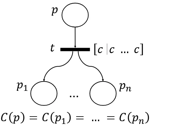
With the aim of developing methods and techniques help in discovering auto-matically and effectively the causes leading a system to misbehave, a prominent concern of research effort has been and is being oriented towards fault diagnosis problem. A general investigation of such a problem considers the type of knowl-edge available. In fact, there are two kinds of diagnostic knowlknowl-edge, shallow knowledge and the so-called deep knowledge. Shallow knowledge refers to empiri-cal knowledge that can be gleaned from past experience with the meant system. It consists of a set of observations of faults assigned to them diagnoses and generally takes the form of an expert system (it is usually acquired by interviewing domain experts and encoded as if-then rules). On the other hand, deep knowledge refers to the knowledge about the system internal structure, components, and their in-teractions. It may be developed from a fundamental understanding of the system in the form of a mathematical model, which allows us predicting its behaviour for any admissible input condition. Up to here, the approaches making use of shallow knowledge are classified as expert-system approaches and model-based approaches in the case of deep knowledge.
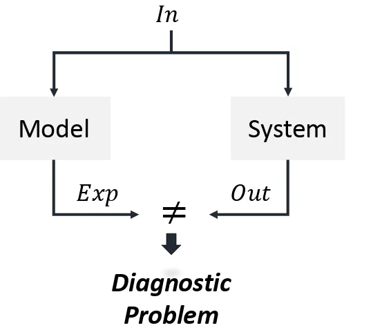
Early in the previous century, diagnosis occurred as one of the most common domains where the expert-system approach was applied; unfortunately, using it for diagnosis of artefacts rather than medical diagnosis became a bottleneck. The acquiring and maintenance of the required knowledge represent cumbersome tasks in the deployment of diagnostic systems. In the late 70’s and instead of using such expert or shallow knowledge (which could be regarded as the experts’ subjective view of the system), the use of deep knowledge (as the objective view of the system) for diagnosis started to be investigated. Since then model-based diagnosis has become a general approach adopted successfully in a variety of application domains, e.g., aerospace, military, transportation, manufacturing and production, ... etc. In this approach, the reasoning process is performed based on a mathematical model of the system behaviour, together with an observation of how the system actually behaves. A problem of diagnosis is then pointed out when there are discrepancies between the gotten observation and the predicted behaviour (using the system model), the idea of the approach is fully presented in
Fig. 2.1.
Model
System
𝐼𝑛 𝑂𝑢𝑡 𝐸𝑥𝑝≠
Diagnostic
Problem
Figure 2.1: A presentation of diagnostic activity
Given the same input value for both the real system and its model. The output of the system (gotten by observation) is compared to the expected one (generated using the system model). For the case of no differences between the obtained results (outputs), it may be assumed that the system works correctly. In case some significant difference of the observed behaviour from the predicted one takes place, it must be stated an inconsistency between the system real behaviour and its model. Here, system misbehaviour is detected, which implies the occurrence of a fault (when assuming the system model is correct).
A model is some description of a system given, in our case, in a formal manner by using a modelling language. For diagnosis, this model can describe the system behaviour in the fault-free case (i.e, correct behaviour), as it can give knowledge about which fault can occur and the consequences it may provoke (i.e, faulty behaviour), and possibly both. A system model is usually component-oriented, where the corresponding system can be viewed as a set of components interacting among each other. This is the case when the model is not designed specifically for diagnosis purposes, thus no information about the system behaviour in the presence of faults is given. Here, a system diagnosis consists of identifying the parts of the system responsible for some unexpected behaviour. Another possible view of the system model could be that describing the causal relationships between faults and symptoms, it exploits by that the system causal behaviour.
2.2
Principles of Model-Based Diagnosis
In this section, a short overview of model-based diagnosis is given. In particu-lar, it reviews the most popular approaches to diagnosis the abductive and the consistency-based. Then, it details a unified framework based on the integration of both approaches for centralized and distributed systems. Here, the first-order logic will be used to formalize the main notions and concepts related to each approach.
2.2.1
Approaches to model-based diagnosis
According to the representation of knowledge about the normality and faults, and then how diagnoses are defined and computed, there are two prevailing approaches to model-based diagnosis, consistency-based [44] and abductive [39].
Consistency-based diagnosis
Back to the seminal paper "A Theory of Diagnosis from First Principles" of Ray-mond Reiter, where he has set the basic notions of diagnostic reasoning based on analysis of inconsistency between the system real behaviour and the predicted one (using its model). In this theory, the system model is already available, it may be constructed for reasons other than diagnosis, as the case of an artefact where the created models during its designing could be exploited for diagnosis.
In this approach, the system description SD can be defined by the pair (BM, COMP S). BM, for Behavioural Model, is a set of first-order formulas defin-ing how the system components are connected and how they normally behave. COMP S = {c1, ..., cn}is a set of constants listing the system components. By
as-suming that all of these components behave correctly, ∀c ∈ COMPS ¬AB(c) (AB for abnormal), the correct behaviour of the system can be formalized as:
BM ∪ {¬AB(c1), ..., ¬AB(cn)}
On the other hand, the current behaviour of the system can be obtained by measuring the values of its observed variables as an observation. This observation can be given as a set of first-order formulas too, let it be OBS. When the system
acts correctly, then it fulfills the consistency of
BM ∪ {¬AB(c1), ..., ¬AB(cn)} ∪ OBS
Whereas, if at least one of the system components becomes faulty, ∃c ∈ COMPS AB(c), it turns out to be inconsistent. In this case, we have a problem of diagnosis, the observation on the system is inconsistent with the assumption above (all components work as expected). A diagnostic problem is then given by
DP = (BM, COMPS,OBS)
It should be noted that the resulted inconsistency is caused by assuming that all components behave correctly, which is in fact wrong. Therefore, the diagnostic process consists in searching for some set of components, a subset of COMP S, that when assumed to be faulty, it brings consistency back explaining the system misbehaviour.
Definition 2.1. A diagnosis for a system with observation, given by (BM, COMP S, OBS), is a minimal set∆⊆ COMPS such that
BM ∪ OBS ∪ {AB(c)|c ∈∆} ∪ {¬AB(c)|c ∈ {COMPS −∆}}is consistent The minimality requirement is strictly necessary, here, to avoid redundant diagnoses. Notice that by changing the assumption ¬AB(c) to AB(c) for certain component c, it leads to regaining consistency between the observed behaviour of the system and the one predicted using its model. In this case, c is assumed to be broken, then∆= {c} is a diagnosis to DP. It is a consistency-based diagnosis, by which explaining inconsistent observations corresponds to restoring consistency. Before moving on, it is worthy to outline the notion of a conflict set, as the key idea of the theory of consistency-based diagnostic reasoning. A conflict set is any subset of components {c1, ..., ck} ⊆ COMPS that, given the observations, cannot
be claimed to be simultaneously correct (at least one of them must be faulty), i.e.,
BM ∪ OBS ∪ {¬AB(c1), ..., ¬AB(ck)}
is inconsistent, besides it is said to be minimal if any of its proper subsets is not a conflict set. Up to here, consistency-based diagnoses can be built by
combining elements from different conflict sets, each diagnosis should have at least a component in common with each conflict set, which leads us to another important concept, that is, a hitting set. We say that H is a hitting set for a collection of sets C if H ⊆ ∪S∈CS such that H ∩ S 6= ; ∀S ∈ C. Again, a hitting set
is minimal if any of its proper subsets is not a hitting set. We end by presenting the basic theorem of Reiter’s theory [44].
Theorem 2.1. ∆⊆ COMPS is a diagnosis for DP = (BM, COMPS, OBS) if and only if∆is a minimal hitting set for the collection of conflict sets forDP.
Abductive diagnosis
The abductive diagnosis approach generally considers the faulty behaviour of the system. In fact, such reasoning is usually adopted in the medical domain. In this case, explaining misbehaviour or a symptom means finding a set of causes that implies logically the symptom itself and not just by being consistent with it, as the case of consistency-based approach. In this respect, the behavioural model of the system describes what happens in case of faults, when the system deviates from its correct behaviour. Therefore, we introduce a set of faulty behaviour modes for each component c as follows: mod e(c) = {m1, ..., mn}, where m1, ..., mn denote the
possible failure modes. Here, the BM of the system contains, besides the structure of the system, a description for each faulty behaviour mode of each component (one of these modes could be the unknown mode with which no model is associated [36]), it is given as implications describing causal relationships between faults and their causes. Notice that due to the absence of the correct behaviour, no discrepancies between the observed and the predicted behaviours could be detected (there is no expected outputs to be predicted). Thus, BM ∪OBS∪{¬AB(c)} remains consistent, unlike the previous approach.
Note that OBS ≡ I ⇒ O, where I denotes the inputs and O denotes the outputs. Since there is no inconsistency to be explained when the expected normal mani-festations are unavailable, diagnostic reasoning is confined to give some account for some observed manifestations. Let CO ⊆ O be a combination of outputs to be explained. An abductive diagnosis for CO is given by∆such that:
BM ∪ I ∪∆is consistent.
* Furthur remarks
As discussed before, consistency-based and abductive diagnosis differ in the representation of normality and faults and in the meaning they give to the term explain. Instead of the abductive view where a component is abnormal if it manifests as it is described in the behavioural model1, in the consistency-based view, a component is abnormal if its observed behaviour deviates from the expected one. that makes the difference between explanations very obvious. In the first approach, a solution attempts to explain why the system reacts as it is observed; while in the second a solution explains why the system exhibits a malfunction. In other words, any computed diagnosis does not exactly explain the observed behaviour of the system. The observed behaviour itself is not important, the significance lies in being different from what is expected. That explains some of the undesirable results when using such an approach (as illustrated in the domain of digital circuits by [23]).
An idea concerning both approaches consists in exploiting knowledge about faults in the consistency-based approach, and knowledge about correct behaviour in abductive approach. In other words, extending component-oriented models to describe the possible faults of the system and their consequences, as well as including descriptions of nominal behaviour in causal models ([38], [51]). In fact, the two approaches were integrated ([22], [13], [18]) and shown to be the extremes of a wide spectrum of possible definitions of diagnosis ranging from a pure consistency-based diagnosis to a pure abductive diagnosis [15].
2.2.2
Unified framework for MBD
In the framework proposed in [15], the diagnostic problem is defined as an ab-duction problem with consistency constraints, where an observation must be entailed by a diagnosis with the satisfaction of some consistency constraints.
1In fact, BM describes, according to the abductive approach, different faulty behavioural
modes. In the discussion above we have assumed, for reasons of simplicity, that only one faulty behavioural mode, noted AB, is modelled.
Here, the correct and faulty behaviours of a system have been represented in a uniform way. As already known, a model of the investigated system is of crucial importance in order to perform a model-based diagnosis. Usually, such a model is developed based on a deep understanding of the system. This understanding can be generally expressed in terms of relationships between the different units or variables of the system. In fact, qualitative models are widely used essentially for diagnostic reasoning, which does not require precise measures over the system, but rather it works in broad ranges of values like absent/present, high/low and so on. In this case, the system variables are characterized by a few discrete values. When such relationships describe the cause-effect transformations among system variables, the system model, besides being qualitative, becomes causal. Indeed, causal knowledge is very useful for diagnosis, in particular, it helps to discover the causal path explaining the made observation.
In terms of causal models, system behaviour can be viewed as a set of states (also entities), describing partially the situations in which the system can be at a given time, connected among them by means of cause-effect relationships. Each of these states ranges over a finite set of values often referred to as admissible-values. According to [14], the system states can be classified, for diagnostic purposes, into:
• Initial-causes: represent system states from which any evolution begins;
• Internal-states: represent non-observable states, usually, as consequences of initial-causes;
• Manifestations: are observable and measured states by which observations would be made.
When dealing with faulty models, initial-causes represent initial perturbations leading the system to misbehave, whereas manifestations represent expected symptoms. In this case, explaining a symptom, an observation in general, consists of finding a set of initial causes implying it.
Up to here, a diagnostic problem consists of the triple DP = (BM, I N IT,OBS), for which BM is the causal model describing the system behaviour, while I N IT denotes the set of initial-causes instances in terms of which an observation OBS would be explained. A solution to DP must predict the observation OBS, as well
as satisfy some consistency constraints. By the way, as already said, according to the unified framework, there is a spectrum of diagnostic problem definitions depending on the selected (sub-)observations to be covered (directly supported) by a diagnosis. A diagnostic problem DP is then defined as an abduction problem as follows.
Definition 2.2. The abduction problem corresponding to DP is given by
AP = (BM, I N IT,〈Ψ+,Ψ−〉)
such that: Ψ+⊆ OBS and Ψ−= {m(x)|m(y) ∈ OBS, x 6= y} (m is a manifestation and x, y ∈ admissible_values(m)).
By considering OBS to be the made observations.Ψ+is a subset of observa-tions to be entailed (covered) by a solution of AP.Ψ− is the set of all possible values that conflict with the made observation (which are known to be absent in the case under examination). It is typically used for consistency checking. A solution to AP is then defined as∆⊆ I N IT for which
∀x ∈Ψ+ BM ∪∆` x ∀y ∈Ψ− BM ∪∆ 0y
∆must predict each parameter inΨ+ and no parameter inΨ−. In other words, a solution to AP must be consistent with all observable parameters while covering a selected group of them.
2.2.3
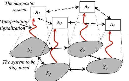
Distributed Model-Based Diagnosis
Generally, when designing a fault diagnosis system one can pursue a centralized, decentralized, or distributed architecture. With the fact that an increasing number of nowadays built systems are concurrent and often distributed, the most suitable architecture when constructing a diagnostic system would be the distributed one. Practically, a distribution of the system model over the diagnosis system can be (referring to [48]):
* semantically according to the type of knowledge, e.g. a separate model of the electrical and of the thermodynamical behaviour of the system.
In this thesis, we focus on the spatially distributed one.
A distributed system S (the one to be diagnosed) is characterized by its struc-ture, it consists of a collection of interacting subsystems S1, ..., Sn(each of which
represents a part of S), that do communicate and cooperate among each other. And with that, a distributed approach of multiple diagnostic agents, where each agent is associated with a specific subsystem, has been argued appropriate [46]. In such an approach, the system model is distributed over the agents, the diagnosis is locally generated and the consistency between the subsystems should be satisfied, by means of communication among agents (agents derive the distributed diagnosis by local calculations and by information exchanges, e.g., [25], [24], [26], [29], [4], [31], [43], [52], and [53]). In that case, each agent Ai is in charge of a subsystem
Si, has its local model, receives the local observations and can exchange limited information with the adjacent agents for consistency checking.
Figure 2.2: A diagnostic system architecture.
Within this view, the initial DP can be formalized as a conjunction of n local diagnostic problems DP =Sn
i=1DPi. Each of these DPi corresponds to a
particular subsystem Si. Notice that each subsystem Si can not be fully
inde-pendent from the other system parts. It interacts with them through different connection elements. By considering these connection elements, a local diagnostic problem DPi would be given by DPi= (BMi, I N ITi, I ni, Outi, <Ψ+i,Ψ−i >). Here,
I ni and Outi correspond to connection elements that are classified into inputs to
Si, that are determined from other subsystems Sj, and outputs from Si to Sj.
Definition 2.3. Given a local diagnosis problem DPi= (BMi, I N ITi, I ni, Outi, <
Ψ+
i,Ψ−i >), a consistent local solution to DPiis a set of assumptions∆i⊆ I N ITi,
such that:
∀m ∈ Out+i ∪Ψ+i : BMi∪ Ini∪∆i` m
∀n ∈ Out−i ∪Ψ−i : BMi∪ Ini∪∆i0n
In order to determine a solution to DP that is globally consistent, the reasoning task needs to be performed in two steps. At first, the agent Aidefines a preliminary
local diagnosis to DPi in absence of any external information from neighbouring
agents. The step that follows consists of checking consistency with neighbouring agents. Each agent Ai must discard its own diagnoses that are not consistent with
those of the neighbourhood. Starting from∆i, agent Ai deduces the instances of
the states corresponding to outputs of Si to be compared with values requested
by neighbouring agents as their inputs. Note that, analogously to the gotten observation, Outi is classified into two subsets Out+i and Out−i. Out+i denotes the
output values that are modelled in BMi and are deduced from∆i; whereas Out−i
holds the modelled values in contradiction with the deduced ones.
2.3
Petri Nets
In about the 1960’s, Petri nets were introduced by Carl Adam Petri in his PhD dissertation as bipartite directed graphs intended for modelling concurrent, asyn-chronous, distributed and/or parallel systems. Petri nets are well-suited tools that offer a clear and precise description of the system’s static structure besides its dy-namics in one net model via the graph structure and the token game respectively. Another interesting aspect about them is that they are designed to assist system analysis, and so different techniques, reachability-based and algebraic-based, have been developed for studying them. Side by side to the formal description and analysis, such nets provide a convenient graphical representation of the investigated system that comprises: places (circles), transitions (rectangles), to-kens (black dots) assigned to places, and arcs as relationships between places
and transitions. The formal definition of Petri net and the relevant concepts are presented in what follows, for further details we address the reader to [35].
Definition 2.4. A Petri net is a 4-tuple N = (P, T, A,W) where:
• P ∩ T = ;,
• P ∪ T 6= ;.
• A ⊆ (P × T) ∪ (T × P).
P is a set of places, T is a set of transitions, A is a set of arcs, and W is a weight function such that ∀a ∈ A : W(a) ≥ 1. In case ∀a ∈ A : W(a) = 1, N is said to be an ordinary PN. In what follows, let X = P ∪ T be the set of nodes (elements) of a Petri net.
Definition 2.5. Given a net N = (P, T, A,W) and x ∈ X . •x = {y|yAx} and x•= { y|xA y} are called the pre and post sets of the node x respectively. The node x is a source if•x = ;, while it is a sink if x•= ;.
Definition 2.6. Given a net N = (P, T, A,W). A marking of N is a function µ : P →
N representing the number of tokens into places. An initial marking is singled out and denotedµ0.
A marked Petri net (N,µ) denotes a Petri net together with its marking.
Definition 2.7. Given a marked Petri net (N,µ). A transition t ∈ T is enabled at a markingµ iff
∀p ∈•t :µ(p) ≥ 1.
Once t is enabled atµ, it may fire producing a new marking µ0(we writeµ[t〉µ0)
such that ∀p ∈ P:
µ0(p) = µ(p) − W(p, t) + W(t, p).
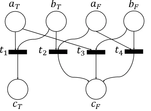
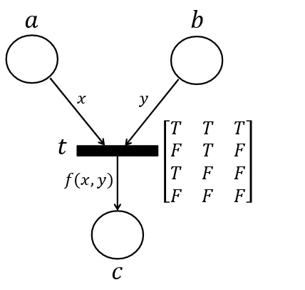
Example 2.1. As an example, let us consider the logical expression a∧b ≡ c, where
a, b and c assume boolean values (T for true and F for false) and ∧ is the logical connective and; c is true only when both a and b are true, it is false otherwise. The expressionc can be described by the Petri net shown in Fig. 2.3. Since a and b can
be set in four different ways, the PN corresponding to c has four transitions, e.g. t1
represents the setting when botha and b are true (given by the places aT andbT respectively), and so the value ofc is also true (given by the places cT).
𝑎
𝑇𝑏
𝑇𝑎
𝐹𝑏
𝐹𝑐
𝑇𝑐
𝐹𝑡
1𝑡
2𝑡
3𝑡
4Figure 2.3: Petri net corresponding to a ∧ b → c
A very useful tool for Petri nets analysis is the reachability graph. As an oriented graph, a reachability graph describes the state space of the system, that means the possible states the system could be in during execution. In fact, reachability can be considered as a fundamental basis for studying the dynamic properties of any system [35]. The firing of an enabled transition will change the token distribution (marking) in a net according to the transition rule. A sequence of firings will result in a sequence of markings. A markingµ is said to be reachable from a markingµ0if there exists a sequence of firings that transformsµ0→ µ.
Definition 2.8. Given a marked Petri net (N,µ0), the reachability set from a
markingµ0, indicated as R(N,µ0) (also [µ0〉), is the smallest set of markings such
that:
• µ0∈ R(N, µ0);
• if µ1∈ R(N, µ0) andµ1[t〉µ2for some t ∈ T, then µ2∈ R(N, µ0).
At the end, we consider the following features:
• Two transitions are said to be concurrent if and only if each time they are both enabled, the firing of one does not prevent the other from being enabled.
• A marked Petri net (N,µ0) is deterministic if and only if ∀µ ∈ R(N,µ0)
∀t1, t2∈ T : if µ[t1〉 and µ[t2〉 then t1and t2are concurrent.
• Given a place p ∈ P, and a marking µ0. The situation whereµ0(p) is said to
be reachable from a marked Petri net (N,µ), write (N,µ) ` µ0(p), iff
µ0∈ R(N, µ) and µ0(p) 6= 0
Coloured Petri Nets
Coloured Petri Net is the expanded form of Classical Petri Net that has the ability of programming with ML programming language. ML is the programming language for AI whose composition with coloured Petri net modelling made it useful for creating recursive functions and different commands on the edges of models. By using Coloured Petri Net, adding operators and multi-set marking is possible, and the best tool for modelling and verification of models is CPN tools (CPN), used in the cases such as security and database systems and also in smart algorithms. In general, the CPN model is a formal model as a mathematical description of syntax and semantics model.
In [28], a full description of CPNs has been provided. In fact, such nets have been introduced in order to address the complexity problem of classical Petri nets (a PN model of a given system tends to become too complex, whether the model size or the analysis, even for a modest-size system). The principle of a CPN model is to extend the notion of token with a colour, we use the notation token colour by convenience. That allows describing similar processes in a uniform and succinct way without losing the ability to distinguish between them. Before giving the formal definition of CPNs we need to know about multi-sets. A multi-set is a set where individual elements may occur more than once.
Definition 2.9. A multi-set m over a set S is a function m ∈ [S → N] denoted
P
• ∀s ∈ S : s ∈ m iff m(s) 6= 0.
• SMS is the set of all finite multi-sets over S.
We can therefore define the following operations to deal with mutlisets. Thus, ∀m, m1, m2∈ SMS and ∀n ∈ N: |m| = P s∈Sm(s). m1+ m2 = P s∈S(m1(s) + m2(s))0s. m16= m2 = ∃s ∈ S : m1(s) 6= m2(s). m16m2 = ∀s ∈ S : m1(s)6m2(s) (defined analogously to>).
Note. In the CPN definition below, we set only the needed parts.
Definition 2.10. A CPN is a 5-tuple N = (Σ, P, T, A, C) where: • P ∩ T = ;, P ∪ T 6= ;.
• A ⊆ (P × T) ∪ (T × P).
• C ∈ [P → 2Σ].
The definition of the sets P, T and A for a CPN is analogous to that for Petri nets. Σ is the set of colour sets. C is a colour function that associates to each place p a colour set (denoted C(p) ∈Σ). That means each place p may hold one or more tokens, each of which carries a colour (data value) belonging to p’s colour set. A marking is a functionµ such that ∀p ∈ P : µ(p) ∈ C(p)MS which defines for
each place a multi-set of colours that are presented into. The firing of a transition leads to moving tokens in the net model. Such tokens are determined by the arc expressions (which consist of typed variables, constants, functions or even operators). The evaluation of an arc expression is a multi-set of colours. Moreover, it can be attached to each transition a boolean expression (with variables) called a guard which specifies the bindings for which it evaluates to true. A binding is an assignment of data values to the free variables appearing in the expression of an incoming arc or a guard of a transition. A binding of a transition can be written in the form: (v1= d1, v2= d2, ..., vn= dn) where f or i ∈ 1..n : vi is a variable and
di is the value assigned to vi. We denote by Ex pr < b > the evaluation of the
expression Ex pr with the binding b.
A transition t is enabled if there is a binding such that:
1. The evaluation result of each of the input arc expressions is present on the corresponding input place;
2. The guard (if any) is satisfied.
When a transition t is enabled at a markingµ such that µ[t〉µ0, the new marking
µ0 is calculated as follows
∀p ∈ P : µ0(p) = µ(p) − E(p, t) < b > +E(t, p) < b > where E(x1, x2) refers to the expression of the arc (x1, x2).
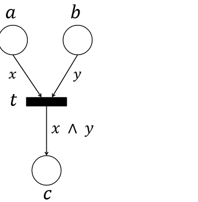
Example 2.2. Back to the previous example. The CPN model corresponding to
the same expression is displayed in Fig. 2.4, whereC(a) = C(b) = C(c) = {T, F}, an expression is attached to each arc remembering that the x and y are variables on a multi-set. Thus the expression x ∧ y states that in case transition t fires, a token of colour x and a token of colour y are destroyed on a and b respectively. Accordingly, the possible settings of the arc expression x ∧ y are T ∧ T, T ∧ F, F ∧ T and F ∧ F.
𝑎
𝑏
𝑐
𝑡
𝑥 𝑦
𝑥 ∧ 𝑦
2.4
PN-Based Diagnosis
It is worth knowing that a system model is of crucial importance in the MBD approaches, thus the use of precise language plays a major role. Petri nets have be-come very well-known tools in this area due to their ability of modelling, validating and verifying a wide range of systems, all in a uniform language. Solving diag-nostic problems using PNs has already been investigated by several researchers, we mention in this regard the works of [8], [47], [3], [42], [33], [54], [2], where the reasoning task is captured by exploiting the classical analysis techniques of PNs.
2.4.1
Brief survey
In fact, several approaches and frameworks have been proposed depending on the system nature and the used formalisms. In the context of Petri Nets, discrete event systems (DES) have gained big efforts. We mention in this regard the work of [6] on the problem of identification and synthesis of the faulty model of a PN in such a way the fault-free system is supposed to be known. The work of [34] investigates the effect of fluidization of PNs on fault diagnosis focusing particularly on untimed continuous PNs. As well, [49] provides a discussion of an online approach for DES fault diagnosis in basis of labelled PNs (an overview of the historical development of DES within PNs can be found in [27]). The work in [7] presents a decentralized approach based on labelled PNs for diagnosing discrete-event systems (DES). It extends the communication protocols defined in [19] for automata to the PN-based approach introduced in [9]. In the same field, the work in[12] deals with the problem of diagnosing DESs based on PNs by introducing an on-line decentralized approach, where the system to be diagnosed is assumed to be observed by a set of sites. Each site is informed with the system structure and the initial marking, whereas the observation is done locally. At the level of each site, a local diagnosis is performed by making use of some integer linear programming (ILP) problem solutions [21]. The work in [54] concerns the identification problem of faulty behaviour in a DES. Based on PNs, the identification process starts by extracting the abnormal behaviour from a given observed sequence, building a non-linear integer programming, then converting it to an ILP, whose solutions identify the
set of faults leading the system to misbehave. We can mention also the work of [37] where a CPN version of the diagnoser introduced in [47] is presented. Such a diagnoser is constructed on the basis of a labelled PN model of the system to be diagnosed. The approach is, then, extended to implement a modular diagnoser for large distributed systems. The work of [32], as an earlier work, exploits CPNs as well for modelling, then diagnosing a BPEL web service, the diagnosis problem is given as inequations system constructed using the evolution equation of PNs, whereas to solve such a problem an algebra algorithm is proposed.
The work with the largest point of contact with this thesis is one quite early published by [42] (then extended by [3]), which addresses the problem of the application of PNs approach to model-based diagnosis. Such a work uses a specific class of PNs called Behavioural Petri Net (BPN), introduced in [1] to represent a system given by its causal behaviour. Moreover, it defines a particular backward reachability analysis method called BW-Analysis to perform the reasoning (di-agnosis) scheme. It exploits two different kinds of tokens, normal and inhibitor, aimed at modelling the truth or falsity of the condition associated with a marked place. A formal description of the approach is as follows.
2.4.2
BPN-based diagnosis
Behavioural Petri Nets
The idea of using PNs to represent a causal model, then verify it, was introduced by Portinale in [40]. It resulted in defining a specific class of PNs, referred to as Behavioural Petri Nets [1], to describe particularly a system’s causal behaviour. One of the main features for which such a net model is defined is that finding an alternative to logical formalisms in such a way that the precise semantics of a causal model can be given in terms of Petri net structure and behaviour. For further discussion about BPNs, a full description can be found in [1].
Definition 2.11. A BPN is a 4-tuple N = (P, TN, TOR, A) such that (P, TN∪
TOR, A) is an acyclic ordinary Petri net with: • ∀p ∈ P(|•p| ≤ 1 ∧ |p•≤ 1|)
• ∀t ∈ TN(|•t| = 1 ∧ |t•| > 0) ∨ (|•t| > 0 ∧ |t•| = 1)
• ∀t ∈ TOR(|•t| ≥ 2 ∧ |t•| = 1)
It should be noticed that a BPN model is safe; that is, any place can hold at most one token2. A transition can be either an And-transition (TN) or an
Or-transition (TOR). And-transitions are intended in the usual way (as conjunctions
of causes); while, Or-transitions are intended to represent the logical connective OR. Thus, an Or-transition has a concession in a marking iff at least one of its input places is marked. The initial marking of a BPN is a safe marking µ0 by
which only source places can be marked.
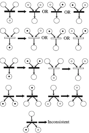
BW-Analysis
Given a BPN, a particular analysis technique called BW-analysis is defined in [1] as a backward analysis method based on reachability. As said previously, such a method uses two different kinds of tokens, normal and inhibitor, aimed at modelling the truth or falsity of the condition associated with a marked place. Thus a marking of a placeµ(p) ranged in {b, w,0}. If µ(p) = b then the place p is marked with a normal (black) token, if µ(p) = w then it is marked with an inhibitor token (white), and if µ(p) = 0 then it is empty, here no constraint is imposed on the condition associated to p (it is unknown).
Starting from a markingµ where only sink places are marked µ(p) 6= 0 ⇒ p•= ;, the BW-analysis makes use of a set of backward firing rules, as illustrated in Fig. 2.5, to determine the set of initial markings from whichµ could be reached. The application of such a method results in a graph whose root node is the markingµ, the leaves are whether initial markings or inconsistent ones, whereas the arcs are labelled with fired transitions. Notice that some of the rules are indeterministic, by that the graph.
Applying BW-analysis to diagnostic problem solving
In terms of BPNs, system behaviour can be represented as follows. Each state’s instance is modelled by a place. Initial-causes instances are represented by source
Figure 2.5: Backward firing rules of a BPN.
places, while manifestations instances are represented by sink ones. Concerning the cause-effect relationships among these instances, they are described by means of transitions. In this case, observation over the system can be described by a final marking by which only sink places, corresponding to manifestations, can be marked.
The BPN diagnostic problem BP N DP corresponding to the logical DP is defined as BP NDP = (N, PI nit, 〈P+, P−〉) where N is the BPN representation of the causal BM, PI nit denotes the set of source places corresponding to initial causes of BM, P+, P−are two sets of sink places representing the observations and thus corresponding respectively toΨ+ andΨ−. The following concepts need to be recalled.
I a markingµ of a BPN is called a final marking if and only if no transition is enabled atµ;
I it is said thatµ covers a set of places Q if and only if ∀p ∈ Q → µ(p) = 1; I whileµ zero-covers the set Q if and only if ∀p ∈ Q → µ(p) = 0
Now the concept of diagnostic solution can be captured by the following theorem whose proof can be found in [41].
Theorem 2.2. Given a BP N DP = (N, PI nit, 〈P+, P−〉), an initial marking µI nit is a solution toBP N DP if and only if the final markingµ of (N,µI nit) covers P+and zero-coversP−.
Up to here, what has been presented is a centralized approach for diagnostic problem solving. In fact, the distributed version of the BPN-based approach has been already investigated by Bennoui in [3] where the system model is given by a set of place-bordered BPNs and the global diagnosis can be achieved through communication between agents each time they accomplish a local diagnosis.
2.5
Discussion
Indeed, BPNs offer a clear and precise language for system description, besides capturing all aspects concerning causal models validation. Nevertheless and as we pointed out in the introduction, a Petri net representation, in general, becomes fairly complex when dealing with real-life systems (even with the smallest size of them). The main reason is that we only have one type of token. As an example, in a mechanical domain, let us consider a state representing an engine temperature. This one can assume high, medium, or low value at a given time. In the corre-sponding BPN model, each of these values is represented by a place. Furthermore, for each one there is an execution path as a subnet to deal with. Notice that the mentioned problem comes up with places and also with transitions. On the one hand, a subset of places belongs to the same modelled state. On the other hand, a subset of transitions shares the same place_domains (both inputs and outputs) and performs the same action with them. Here, we use the term place_domain to denote the set of places corresponding to a state’s values.
Usually, such kind of problems can be faced by turning to high-level net classes, and particularly the Coloured Petri Net one, since it represents the structural
folding of classical PNs (of course, when the places’ colour-sets are finite). Hence, a mapping between a BPN and a CPN can be informally defined as follows.
I We replace a set of places {p1, ..., pn}belonging to the same place_domain by
a single place p, as long as, we attach to p the colour set {c1, ..., cn}in such
a way that each colour ci refers to a place pi. Here, a token in the place
p represents the fact that the corresponding state to p assumes the value modelled by the colour carried by such token.
I We replace a set of transitions {t1, ..., tm} having the same place_domains
for both inputs and outputs by a single transition t, which may fire in m different ways each of which corresponds to a transition ti.
I Again, a markingµ of a CPN is a safe marking, each place can hold at most one token at a time. Obviously, within an initial markingµ0, only the source
places can be marked.
Unfortunately, such criteria are still deficient. They lack a full representation of Or-transitions. Recall that an Or-transition is enabled in a marking if at least one of its input places is marked. An all set proposal consists of adding new transitions and inhibitor arcs3 for that, however, we get again involved in the complexity problem, getting more places and transitions.
Taking up the diagnostic problem again where the reasoning task should be accomplished by a backward analysis, which can be seen as a forward one on the inverted net model. Instead of classical PNs where such a process needs only an inversion of the arcs’ direction, in terms of CPNs, it can be realized in two steps:
1. Inversion of arcs’ direction; and
2. CPN expressions (guards or those associated with arcs) inversion.
In this respect, many attempts have been made such as [11], [20] and not very ear-lier [5]. The work presented in [5] consists in proposing a backward reachability analysis based on an inverted CPN, which can be obtained by means of structural
3An inhibitor arc connects a place p to a transition t in such a way that it disables the
transition t when the input place p is marked. Notice that no tokens can move through an inhibitor arc when the transition fires.
transformations on the original net model. Here, let us get to a significant issue concerning the analysis task within CPNs. We have mentioned that a transi-tion may fire in several ways, besides the use of arc expressions to determine the involved token colours when it fires. Although such expressions are linear functions in general, the inversion process may be impossible for some cases and hard for others. Of course, we do not account the trivial cases where functions are of one input argument. Rather, the complexity arises in case of multi-input arguments, the reasoning process needs generally exponential time, besides being not adequate to our aims.
To simplify the analysis task, we propose using matrices as labels for transi-tions where the different firing ways are determined with. Each line of the matrix corresponds to a way of firing and determines the involved token colours. As well, each column corresponds to a place and shows the meant token colours (whether consumed or produced) by this transition. In fact, this proposal is the key feature of a particular class of CPNs called CBPNs, as a folding of BPNs introduced in [42]. It should be noticed that we do not intend to neglecting the arc expressions, but they will be used as typed variables and selective expressions.
2.6
Conclusion
This chapter has reviewed the main concepts and notations related to fault diagno-sis problem within a model-based reasoning view for centralized and distributed systems, as will be used in this thesis. Also, some definitions concerning Petri nets that would be useful throughout the thesis have been recalled. Then, and since we are inspired by the works presented in [42] and [3], they are both detailed to some extent; whereas a brief survey is considered for the use of PNs in the general context of model-based diagnosis.
The chapter has ended by discussing the major weakness related to PN-based approaches in general that is the complexity problem in terms of net representation when dealing with real systems. As well as, the problem concerning the backward analysis of a CPN model where an inversion of the net expressions (the ones attached to arcs) is recommended.
The following chapter aims at presenting the first contribution of this thesis, in which we make use of the CPN models to tackle the first problem, so the system model becomes more reducible. Besides, using matrices attached to transitions to describe explicitly their firing ways instead of being implicit in arcs expressions. In fact, this gives rise to a particular model based on CPNs named Coloured Behavioural Petri Net.
C
H
A
P
3
C
OLOURED
B
EHAVIOURAL
P
ETRI
N
ETS
This chapter provides a full description about the structure and dy-namics of Coloured Behavioural Petri Nets in order to represent the causal behaviour of the system under study. As well as, an illustra-tive example is discussed to touch on the very related concepts. The chapter ends by a BPN-CBPN translation procedure together with an application example and a proof of correctness.
3.1
Introduction
Petri net models are well-known useful tools that offer a clear and precise descrip-tion of the system under study. However, the use of one type of token provokes a salient problem that is the net representation, which becomes fairly complex even for small systems. Coloured Petri Nets have been introduced, as high-level net models, to simplify the PN model structure. Generally, high-level Petri nets have been widely used in both theoretical analysis and practical modelling of various systems. The main reason for the success of this class of net models is that they make it possible to obtain much more succinct and manageable descriptions than can be obtained by means of classical Petri nets. Besides, they still offer a wide range of analysis methods and tools.
3.2
Coloured Behavioural Petri Net models
Coloured Behavioural Petri Nets (CBPNs) denote a particular class of CPNs with the following features. Each place describes a system state, and so its colour set corresponds to the set of such a state admissible values, provided that being marked with one token colour at a time. A token colour in a place means that the state corresponding to such a place assumes the value described by such a colour. A matrix is attached to each transition to define the different ways the transition may fire, and so each row corresponds to a classical PN transition; while each column corresponds to a connected place and shows the involved token colours when it gets fired. Accordingly, a transition input arc is labelled with a typed variable, while with a selective function if it is an output one. Generally, this is all about the static structure of a CBPN, whereas its dynamic behaviour or the token game can be expressed via the following rules:
Enabling of a transition:
A transition is enabled if a combination of its input places markings formalizes a sub-row (by considering only the columns of these places) of its firing ways matrix.
Firing of an enabled transition:
An enabled transition may fire. If a transition fires, it destroys one token colour on each of its input places and creates one token colour on each of its output places according to a certain row of its firing ways matrix.
3.2.1
Structure of CBPNs
Definition 3.1. A Coloured Behavioural Petri Net is a 6-tuple N = (Σ, P, T, A, C, FW) where:
• (Σ, P, T, A, C) is a Coloured Petri Net. • FW : T −→ M ATn,m(Σ∪ {ε}).
• A+(transitive closure of A) is irreflexive.
Since CBPN models can be considered as the CPN-version of causal models, the set of places can be partitioned into three subsets: Initial causes I c, Manifestations Mn, and Internal states I s. Thus,
P = I c ] Mn ] Is
such that:
* I c = {p|p ∈ P, •p = ;}, * Mn ⊆ {p|p ∈ P, p•= ;}, and
* I s = P \ (I c ∪ Mn).
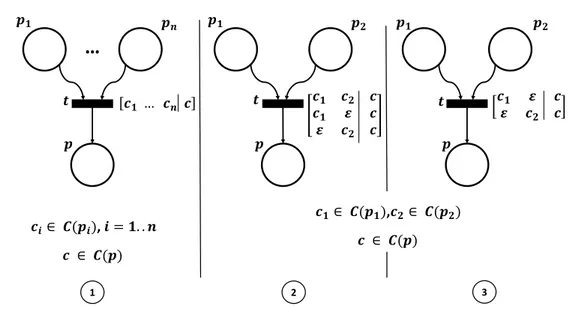
Given a transition t ∈ T with n firing ways, that means the number of transi-tions for which t may be unfolded in a classical PN, and m places with which it is connected (m = |•t| + |t•|).
Firing ways matrix:
A t’s Firing Ways matrix FW = [ci j] is an n × m matrix of colours ci j ∈Sω∈Σω
including the empty colourε. The FW matrix contains a row for each firing way and a column for each connected place. Thus, the ci jconsists of the colour removed
Empty colourε:
Since the FW matrix contains only colours, while a place may have an empty markingthe empty set, which is actually a set, can not be included. Thus, we are imposed on introducing a particular colourε that we call empty colour to stand for the empty set inside a matrix (its utility will be shown later).
A transition t, besides being associated with a firing ways matrix, can be ranged as a fork transition if |t•| > 1; or a join transition if |•t|>1. In case t is a
fork transition then it is intended to split the meant input token colour (where multiple consequences are present). Here, the colours belonging to the same row must be similar.
...
𝑝
𝑝
𝑛𝑝
1𝑐 𝑐 … 𝑐
𝑡
𝐶 𝑝 = 𝐶 𝑝
1= … = 𝐶 𝑝
𝑛Figure 3.1: Fork transition
While if it is join, we meet three possible cases of use.
• The first is as usual when t is a conjunction of causes. In this case, t becomes enabled if all its input places are marked (empty markings are excluded).
• The second consists of the logical Or where t becomes enabled if at least one of its input places is marked. For the sake of simplicity, we often suppose that t has at most two input places. The use of such kind of transitions allows us to model situations in which a particular instance of a state can be determined by alternative causes while keeping safeness.
• The last one is a particular case of the second, it consists of the exclusive Or, where t becomes enabled if and only if just one of its input places is marked.
…
𝒄𝟏 … 𝒄𝒏 𝒄 𝒄𝒄𝟏 𝒄𝟐 𝒄 𝟏 𝜺 𝒄 𝜺 𝒄𝟐 𝒄 𝒄𝟏 𝜺 𝒄 𝜺 𝒄𝟐 𝒄 𝒑𝟏 𝒑𝟏 𝒑𝟏 𝒑𝟐 𝒑𝟐 𝒑 𝒑 𝒑 𝒕 𝒕 𝒕 𝒑𝒏 𝒄𝒊∈ 𝑪(𝒑𝒊), 𝒊 = 𝟏. . 𝒏 𝒄 ∈ 𝑪(𝒑) 𝒄𝟏∈ 𝑪(𝒑𝟏),𝒄𝟐∈ 𝑪(𝒑𝟐) 𝒄 ∈ 𝑪(𝒑) 1 2 3Figure 3.2: Possible cases of join transition
Finally, the FW(t) can be decomposed into FW inn×|•t|and FW outn×|t•|as the
input and output sub-matrices respectively. Such a decomposition is quite useful in the analysis phase.
𝒇𝒘𝟏
𝒇𝒘𝒏
⋮
𝒑𝟏 … 𝒑𝒊 𝒑𝒊+𝟏 … 𝒑𝒎
𝑭𝑾
𝒊𝒏𝑭𝑾
𝒐𝒖𝒕Figure 3.3: FW-matrix decomposition
Note. The irreflexivity of A+ is reasonable since we are dealing with the causal behaviour of a system without considering temporal aspects.
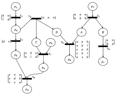
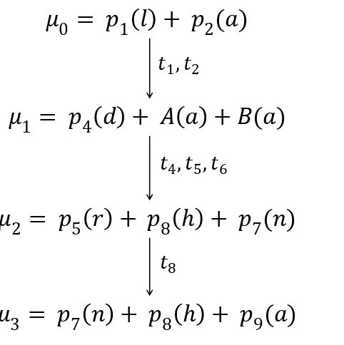
Example 3.1. In terms of the previous example, Fig. 3.4 depicts the CBPN version