A Unified Productivity-Performance Approach Applied to Secondary Schools

A Uni…ed Productivity-Performance Approach Applied to

Secondary Schools

Laurens Cherchye

, Kristof De Witte

and Sergio Perelman

October 27, 2017

Abstract

We introduce a novel and simple diagnostic tool to improve the performance of public services (e.g. in health, education, utilities and transportation). We propose a method to compute perfor-mance/productivity ratios, which can be applied as soon as data on production units’ outcomes and resources are available. These ratios have an intuitive interpretation: values below unity indicate that better outcomes can be attained through weaker resource constraints (pointing at scarcity of resources) and, conversely, values above unity indicate that better outcomes can be achieved with the given resources (pointing at unexploited production capacity). We demonstrate the practical usefulness of our methodology through an application to secondary schools in the Netherlands. In this application, we also account for outlier behavior and environmental e¤ects by using a robust nonparametric estimation method. Our empirical results indicate that in most cases schools’ performance improvement is a matter of unexploited production capacity, while scarcity of resources is a lesser issue.

Keywords: Performance; Productivity; Resource constraints; Secondary schools.

We are grateful to participants of the 2015 EWEPA conference in Helsinki, the Economics in Education Workshop at Maastricht University, E¢ ciency in Education workshop in London, VII EFIUCO at Universidad de Córdoba, Seminar participants at University of Lille, Knox Lovell, Ernest Reig, Hervé Leleu, and Finn Førsund for useful comments.

y_{Center for Economic Studies, University of Leuven. E. Sabbelaan 53, B-8500 Kortrijk, Belgium. E-mail:}

lau-rens.cherchye@kuleuven.be. Laurens Cherchye gratefully acknowledges the European Research Council (ERC) for his Consolidator Grant 614221.

z_{Leuven Economics of Education Research, Faculty of Economics and Business, KU Leuven, Naamsestraat}

69, 3000 Leuven, Belgium. E-mail: Kristof.dewitte@econ.kuleuven.be. Top Institute for Evidence Based Ed-ucation Research, Maastricht University, Kapoenstraat 2, 6200 MD Maastricht, the Netherlands. E-mail: K.dewitte@maastrichtuniversity.nl. Kristof De Witte acknowledges …nancial support from the Horizon 2020 program through the EDEN project (Economics of Education Network).

x_{Université de Liège, Department of Economics, 7, Bd Rectorat (B31); LIEGE 4000 (Belgium). E-mail:}

1

Introduction

One of the major di¢ culties in the provision of public services (e.g. in health, education, utilities and transportation) is for the principal to identify underperformance and its origin. It is for this reason that benchmark methodologies such as frontier analysis have become popular in the literature on public sector evaluation (Fried et al., 2008). Basically, two di¤erent approaches have been used in benchmarking applications. The …rst approach focuses on performance measurement that exclusively evaluates the general outcomes (e.g. population coverage, quality of service provided and inequality issues), without taking into account resource/input constraints. The second approach, which is the most popular one in the applied literature, concentrates on the measurement of productivity, i.e. output performance that explicitly incorporates input constraints.1

One essential di¤erence between these two approaches relates to whether or not resource constraints are taken into account. We may also argue that both approaches provide a partial analysis, which may thus give incomplete and potentially misleading information. First, performance scores, also known as measures of e¤ectiveness, tell us to which extent targets are ful…lled, but they do not inform us if the service provided is produced at full capacity. Second, productivity scores show whether or not the service is supplied e¢ ciently (by exploiting the available production capacity in an optimal way), but they do not tell us to which extent the general outcome targets are achieved. The main reason behind this incompleteness is data availability. Very often data on outcomes and resources are not observable simultaneously, or they do not match perfectly for the production units under observation (Pestieau, 2009; Lefebvre et al., 2017).

Our paper connects to the literature that discusses the intertwining of e¢ ciency and e¤ectiveness (a review is provided in Førsund, 2017). Up to now, most studies consider the case in which the link between outcomes and resources is not directly observable, basically because other factors out of the control of public services a¤ect outcomes.2 _{Therefore, they proceed in a two-step model. In a}

…rst step, they compute e¢ ciency at the public service level using outputs and inputs as in a normal production process and, in a second step, e¤ectiveness is computed at a more aggregated level using outcomes as targets and public service outputs as resources.

This paper provides a unifying framework that …lls this informational gap between performance and productivity measures. Our main contribution is threefold. First, we show that when data on outcomes and resources are available for a large sample of service production units (called Decision Making Units (DMUs) in what follows), both performance and productivity scores are computable by using an appropriate frontier approach. Second, we propose a novel and simple framework to evaluate the importance of resource constraints. As we will demonstrate in the next section, a perfor-mance/productivity ratio below unity indicates that better outcomes can be attained by weakening the resource constraints. In other words, scarcity of resources hampers output performance. On the contrary, a performance/productivity ratio above unity indicates that better outcomes can be achieved with the same resources. This mainly signals unexploited production capacity rather than scarcity of resources. Third, we apply the suggested approach to a representative sample of secondary schools in

1_{For an overview, see Cherchye et al (2007).}

2_{Among factors a¤ecting public service performance, De Witte and Geys (2013) emphasize the role of consumers’}

the Netherlands, for which we have exceptionally rich data, covering most outcome and input/resource dimensions, with identical de…nitions of the variables. This application will demonstrate the useful of our method to guide policies.

The remainder of the paper is organized as follows. In Section 2 we present the theoretical measures of productivity and performance. In Section 3 we show that these measures can be operationalized by solving linear programs of the DEA (Data Envelopment Analysis) form. In particular, we use the robust and conditional DEA form which accounts, respectively, for outlying observations and the operational environment. Section 3 also introduces dual representations of the productivity and performance measures, which gives these measures an additional interpretation in terms of “bene…t-of-the-doubt”weighting. Section 4 introduces the data of our empirical application to secondary schools in the Netherlands. In this application, we will account for outlier behavior and environmental e¤ects, which are essentially resources out of schools’ control, by using a robust conditional nonparametric (DEA) order-m approach. Section 5 presents our empirical results. These results will indicate that, in most cases, school performance improvement is a matter of unexploited production capacity (technical e¢ ciency), while resource constraints are a lesser issue. Using quantile regressions, we provide evidence on the characteristics of schools with unexploited capacity and schools with resource constraints. A …nal section concludes.

2

Productivity, performance and resource constraints

We …rst introduce our theoretical measures of productivity and performance. The basic di¤erence between these two measures pertains to whether or not resource constraints are taken into account when evaluating the possibility to expand outcomes.3 _{We then also introduce a measure that allows}

us to identify either possible outcome gains when resource constraints are weakened or, alternatively, unexploited production capacity for the resources that are available.

2.1

Productivity

We consider Decision Making Units (DMUs) that use an N -dimensional resource vector x 2 RN +

to produce an M -dimensional outcome vector y 2 RM

+. Productivity relates the resources to the

outcomes. In what follows, we evaluate the productivity of DMU E, which uses the resources xE to

produce the outcomes yE: We want to measure the productivity of DMU E in relative terms (also

referred to as technical e¢ ciency), which compares DMU E’s productivity to the maximum attainable productivity for the given state of technology. To this end, we consider the production possibility set P , which contains all combinations of resources and outcomes that are technically feasible (including (xE; yE)). Formally,

P = f(x; y) jx can produce yg.

Throughout, we will assume that the production technology satis…es the technical properties that are needed for our following productivity and performance measures to be well-de…ned. In particular,

3_{We adapt the traditional approach, applied to …rms production, to the particular case of public services. For this}

we assume that it is characterized by constant returns-to-scale, i.e.4

if (x; y) 2 P , then ( x; y) 2 P for 0, (1) free disposability of resources and outcomes, i.e.

if (x; y) 2 P , then (x0; y0_{) 2 P for x}0 xand y0 y, (2) and convexity, i.e.

if (x; y) 2 P and (x0; y0_{) 2 P ,} (3) then ( x+ (1 ) x0; y+ (1 ) y0_{) 2 P for 1} 0.

In practice, we typically do not observe the true production set P . Empirical production analysis starts from an observed set of T DMUs, with resource vector xtand outcome vector ytfor every DMU

t 2 f1; :::; T g. This de…nes the set of observations

X = f(xt; yt) jt 2 f1; :::; T gg:

The nonparametric approach to production analysis (see, for example, Afriat (1972) and Varian (1984)) adopts the basic assumption

X P: (4)

Essentially, this assumes that resources and outcomes are measured without error. Obviously, this is an overly strong hypothesis in many practical situations. Therefore, while we maintain the assumption to simplify our theoretical exposition, we will relax it in our following empirical application (see Section 3.3, where we present the robust estimation method that we will use).

When assuming constant returns-to-scale, free disposability and convexity, we can build the em-pirical set b P = f(x; y) jx XT t=1 txt, y XT t=1 tyt, t 0g. (5)

It can be shown that this set bP is the smallest set consistent with our technological assumptions in (1), (2) and (3), and our empirical assumption in (4) (see, for example, Charnes, Cooper and Rhodes (1978) and Banker, Charnes and Cooper (1984)). As such, it provides a useful empirical approximation for the true but unobserved set P .

Using this, the relative productivity (or technical e¢ ciency) of DMU E is captured by the degree measure

P rodE= min

2Rf j xE;

yE

2 bP g: (6)

Intuitively, for the possibility set bP , the measure P rodEcaptures the maximum (proportional)

expan-4_{We remark that we may also have used alternative returns-to-scale assumptions. One motivation for assuming}

constant returns-to-scale is that it allows for an intuitive (dual) interpretation of our productivity-performance measures in terms of “bene…t-of-the-doubt” weighting, which we explain in Section 3.2. Another motivation, more practical, is that outcomes and resources will be generally represented by indicators, ratios or per-capita values, as in the example presented in next sections.

sion of the outcome yEfor the given resource xE. Clearly, for an observed DMU E (i.e. E 2 f1; :::; T g

and (xE; yE) 2 bP ) we have 0 P rodE 1. Generally, higher values for P rodE indicate a higher

degree of relative productivity (i.e. less possibility to expand outcomes for the given resource). We also say that DMU E is “technically e¢ cient” if P rodE = 1.

2.2

Performance

Performance evaluation disregards resources and only considers outcomes. Put di¤erently, in terms of our above resource-outcome framework, it implicitly assumes that all DMUs can use the same resources. Performance di¤erences between DMUs are solely de…ned in terms of outcome di¤erences, because di¤erences in resource/input constraints are ignored.

To formalize this basic di¤erence between productivity and performance measurement, we consider DMUs with resources normalized at unity. Following Lovell, Pastor and Turner (1995), we can inter-pret this (normalized) resource unit as representing a DMU’s apparatus to achieve its outcome goals, a system which we refer to as the DMU’s “helmsman” (a concept also used by Koopmans (1951)).5

This system may vary across DMUs, but this variation is viewed as irrelevant for the objective of per-formance evaluation, which only considers the outcomes achieved and not the size of the underlying resource system.

Using this idea, the relevant set of observations is

X0_{= f(1; y}t) jt 2 f1; :::; T gg:

which has a similar interpretation as the set X used above, except that now each (helmsman) resource is set equal to one. Using the same technology assumptions as before (constant returns-to-scale, free disposability and convexity), the empirical production set relevant for outcome performance evaluation is given as c P0_{= f(1; y) j1} XT t=1 t, y XT t=1 tyt, t 0g. (7)

Then, the relative performance of DMU E is de…ned as P erfE = min

2Rf j 1;

yE

2 cP0_{g; (8)}

which looks for the maximum outcome expansion when ignoring di¤erences in resource constraints. Like before, for an observed DMU E we have 0 P erfE 1, and higher values for P erfE indicate a

higher degree of relative performance.

5_{See also Lovell and Pastor (1999) for a detailed discussion on productivity measurement with constant input. Lovell,}

Pastor and Turner (1995) used the helmsman interpretation in the context of macroeconomic policy evaluation. Here, we use the same idea in the context of output assessments of micro-DMUs. As a speci…c example, our following empirical application will use the idea for a school performance assessment that focuses on educational outputs per pupil.

2.3

Resource constraints and unexploited capacity

We can distinguish three scenarios when comparing the measures P rodE and P erfE. In the …rst

scenario, we have

P rodE> P erfE:

Thus, the maximum outcome expansion without constraints (captured by P erfE, which ignores

re-source variation) exceeds the maximum outcome expansion with rere-source constraints (captured by P rodE, which …xes the resource xE). This suggests that DMU E can mainly gain in terms of

out-come performance by weakening its resource constraints: The opposite scenario occurs if

P rodE< P erfE:

This inequality reveals that ignoring the resource variation across DMUs actually improves DMU E’s outcome performance. In a sense, the DMU “bene…ts” when we disregard resource variation, which suggests that the DMU does not fully exploit its production capacity (given the resources that it controls). There is speci…c potential for outcome expansion even without additional resources.

The …nal scenario pertains to a situation where

P rodE= P erfE:

Intuitively, the maximum outcome expansion without constraints exactly equals the maximum out-come expansion with resource constraints. In this case, weakening DMU E’s resource constraints will not contribute to a better outcome performance, but ignoring the DMU’s resource constraints does not improve its production assessment either. Comparing the measures P rodE and P erfE does not

speci…cally suggest a particular strategy (i.e. additional resources or better capacity use) to increase outcome performance. Clearly, if P rodE= P erfE= 1, then DMU E is technically e¢ cient and, thus,

it can only improve performance by additional resource (i.e. weaker resource constraints) or technical change which shifts the frontier up. However, P rodE = P erfE < 1 reveals that better capacity use

can also lead to performance gains (because P rodE< 1).

Thus, the di¤erence between P erfE and P rodE can reveal interesting information regarding

spe-ci…c outcome gains from weakened resource constraints (…rst scenario) or unexploited production capacity (second scenario). We can distinguish between the di¤erent scenarios by using the ratio measure

RE=

P erfE

P rodE

.

The three scenarios discussed above correspond to RE < 1; RE > 1 and RE = 1, respectively.

Greater deviations of RE from unity indicate either more outcome gain to be expected from weaker

resource constraints (if RE< 1) or, alternatively, a greater degree of unexploited production capacity

or technical ine¢ ciency (if RE > 1). In case RE = 1;there might still be a problem of unexploited

production capacity if P rodE= P erfE< 1:

The following example illustrates the measures P erfE, P rodE and RE for a simple setting with

only three DMUs, one resource and one outcome. To better articulate the basic intuition, the three DMUs achieve either P erfE = 1 or P rodE = 1 (or both). Of course, this intuition carries over

to situations with P erfE < 1 and P rodE < 1: In such situations, RE < 1 particularly suggests

increasing outcome performance by additional resources (i.e. a weaker resource constraints), while RE > 1 mainly indicates possibilities of outcome expansion by better using the available resources

(i.e. improved capacity use).

Example 1 Suppose a set of observations with 3 DMUs (T = 3) that use a single resource (N = 1) to produce a single outcome (M = 1),

X = f(5; 5) ; (10; 10) ; (20; 10)g: Correspondingly,

X0_{= f(1; 5) ; (1; 10) ; (1; 10)g:} This gives the results

P rod1 = 1; P rod2= 1; P rod3= 0:5, and

P erf1 = 0:5; P erf2= 1; P erf = 1:

Given this, we also obtain

R1= 0:5; R2= 1; R3= 2.

We conclude that DMU 1 can improve its outcome performance by increasing its resources (because R1 < 1). Given that this DMU is technically e¢ cient (i.e. P rod1 = 1), weakening its resource

constraint is the only possibility to achieve a better outcome performance. By contrast, DMU 3 has potential to improve its outcome performance even without additional resources, by better exploiting its available capacity (because R3< 1).

3

Operationalization, duality and robust estimation

In this section, we show that the measures P rodEand P erfE(and, thus, also RE) can be computed by

simple linear programming. This is particularly convenient from a practical point of view. The linear programs are of the form used in the nonparametric approach for production frontier analysis that is known as Data Envelopment Analysis (DEA, after Charnes et al., 1978; see also Fried et al., 2008, for a more recent account of the DEA literature). Attractively, the dual representations of these linear programs also reveal an interesting additional interpretation of our productivity and performance measures. In particular, they show that the measures can be given an intuitive interpretation in terms of “bene…t-of-the-doubt” weighting (see also Cherchye, Moesen, Rogge and Van Puyenbroeck, 2007). Finally, we will show how we can account for outlier behavior and environmental e¤ects by using a robust and conditional estimation method that has been proposed in a DEA context.

3.1

Linear programming formulations

Productivity. As a …rst step, we note that the constant returns-to-scale assumption makes that we can re-write productivity measure (6) as

P rodE= min

2Rf j ( xE; yE) 2 bP g; (9)

Using bP instead of P in this expression de…nes the empirical estimate [P rodE. By combining (5)

and (9), we obtain that this measure can be calculated as the outcome of a linear program: [

P rodE = min (Prod_LP)

s.t xE XT t=1 txt, (Prod_1) yE XT t=1 tyt, (Prod_2) t 0 t 2 f1; :::; T g; free.

Performance. Similar to before, we use that performance measure (8) can be written equivalently as

P erfE= min

2Rf j ( ; yE) 2 cP

0_{g: (10)}

Taken together, (7) and (10) de…ne the empirical measure [P erfE as the outcome of a linear

program:

[

P erf_E = min (Perf_LP1)

s.t XT t=1 t, (Perf_1) yE XT t=1 tyt, t 0 for all t 2 f1; :::; T g; free.

In a …nal step, we can drop the variable and the constraint (Perf_1) as redundant, which leads to the following equivalent formulation:

[ P erf_E = minXT t=1 t (Perf_LP2) s.t yE XT t=1 tyt, (Perf_2) t 0 for all t 2 f1; :::; T g.

3.2

Dual representations

Productivity. Let the vectors pE 2 RN+ and wE 2 RM+ represent the shadow prices for the

follows:

[

P rodE = max wEyE (Prod_LP3)

s:t: pExE = 1;

wEyt pExt 0 for all t 2 f1; :::; T g;

pE 2 RN+, wE 2 RM+:

It is easy to verify that this allows us to de…ne [P rodE as

[ P rodE= max pE2RN+, wE2RM+ wEyE pExEj wEyt pExt 1 for all t 2 f1; :::; T g ;

which implies a speci…c interpretation for [P rodE as the ratio of a weighted outcome sum over a

weighted resource sum. A particular feature is that the resource and outcome weights are chosen so as to maximize this ratio, which e¤ectively gives the “bene…t-of-the-doubt” to the evaluated DMU E.6

Next, the normalization constraint (wEyt

pExt 1) imposes that the maximum attainable productivity

ratio over the sample of T DMUs equals unity. This feature e¤ectively yields an intuitive degree interpretation for [P rodE: using the weights wEand pE de…ned by the program (using

bene…t-of-the-doubt), it represents DMU E’s input-outcome ratio (at most equal to unity) as a proportion of the best achievable ratio in the observed sample of DMUs (which is …xed at unity).

Performance. Interestingly, we can derive an analogous bene…t-of-the-doubt interpretation for our performance measure [P erf_E. Following our previous exposition, the basic di¤erence is that resource constraints are ignored in the evaluation exercise.

Similar to before, we let vE2 RM+ represent the shadow prices for the constraint (Perf_2). Then,

the dual of the program (Prod_LP) is de…ned as follows: [

P erf_E = max vEyE (Perf_LP3)

s:t:

vEyt 1 for all t 2 f1; :::; T g;

vE 2 RM+:

In short, we thus obtain [

P erfE = max wE2RM+

fvEyEjvEyt 1 for all t 2 f1; :::; T gg ;

which represents [P erf_E as a weighted sum of outcomes. Once more, the weights are chosen to

6_{We remark that the ratio formulation of [P rod}

E actually expresses this measure as maximizing “pro…tability” (i.e.

revenue over cost), a concept that is often used in the literature on productive e¢ ciency measurement (see, for example, Grifell-Tatjé and Lovell (2015)).

maximize this sum, which implies bene…t-of-the-doubt weighting. In this case, the normalization constraint (vEyt 1) imposes a maximum outcome sum value of unity for the sample of T DMUs,

which again provides an intuitive degree interpretation to the measure [P erf_E.

3.3

Robust and conditional estimation

Robust estimation. As discussed in Section 2.1, so far we have assumed that resources and out-comes are measured without errors. Obviously, this assumption may be problematic in empirical applications. As measurement errors can shift signi…cantly the production set bP ; they can bias [P rodE

and [P erf_E: Removing the DMUs with measurement errors from bP is usually not an option, mainly because of the following two reasons. First, we often do not know which observations are prone to measurement errors. Second, by simply dropping the observations with outlying values for resources and outcomes we might in fact falsely remove the most interesting observations from the sample.

Cazals et al. (2002) and Daraio and Simar (2005) proposed a method to mitigate the in‡uence of outlying observations and/or observations with measurement errors in applications using the Free Disposal Hull model (i.e., DEA without convexity constraint). Daraio and Simar (2007) extended this to DEA. This method is readily adapted to our productivity and performance measures. In particular, we estimate [P rodE and [P erfErelative to an empirical production set bPmthat is based on

a strict subset of m observations that is drawn (randomly and with replacement) from the observations t 2 f1; :::T g with xt xE: Let us denote the resulting estimates as [P rod

b

E;mand [P erf b

E;m: Then, we

redo this estimation of [P rodb_E;mand [P erfb_E;ma large number of times (say B times, with B > 2000), and we average these B productivity and performance estimates. The obtained averages [P rodE;mand

[

P erf_E;m are called robust order-m e¢ ciency estimates. Basically, they are robust because outlying observations and observations with measurement errors will typically not de…ne the empirical set bPm

in every draw b. Thus, we have e¤ectively mitigated their in‡uence.

As a …nal remark, it is also possible that the evaluated observation E does not belong to the set bPm: As an implication, the values of [P rodE;m and [P erfE;m may well exceed 1. If this is the

case, we label DMU E as “super-e¢ cient”. Basically, a super-e¢ cient DMU is (on average, over the B draws) better performing than the m randomly drawn observations. It is interesting to observe that the robust and deterministic estimates will converge as m ! 1 (i.e. [P rodE;m ! [P rodE and

[

P erf_{E;m ! [}P erf_E): The parameter m serves as a trimming value, which allows us to tune the percentage of super-e¢ cient observations. In our next application, we will follow Daraio and Simar (2005) to …x m at its value for which the marginal decrease in the fraction of super-e¢ cient observations becomes su¢ ciently small (see Appendix 1 for details).

Conditional and robust estimation. A second issue related to the practical implementation of the programs (Prod_LP3) and (Perf_LP3) concerns inter-DMU heterogeneity in terms of production environments. Clearly, DMUs that can operate in a favorable environment have an advantage; the environment works as a substitutive input, and [P rodE;m and [P erfE;mwill be upward biased.

Con-versely, DMUs working in an unfavorable environment will have to put more e¤orts as the environment works as a substitutive output. In what follows, we assume that a DMU’s operational environment is summarized by the s-dimensional vector z 2 RS

Daraio and Simar (2005, 2007) suggest to include the operational environment by extending the robust order-m procedure of Cazals et al. (2002). Like before, the re…ned procedure draws the m observations with replacement from the observations t 2 f1; :::T g with xt xE. But now it

attaches to each observation a particular probability, which is de…ned on the basis of a multivariate kernel function around zE (which characterizes the environment of DMU E). Basically, observations

which are more similar to DMU E in terms of their operational environment are drawn with greater likelihood. Similar to before, a given draw b of observations de…nes an empirical production set bPZ

m,

for which we can compute the estimates [P rodZ;b_E;m and [P erfZ;b_E;m. Again, we redo this B (> 2000) times to obtain [P rodZE;mand [P erf

Z

E;m. It follows that these so-called “conditional robust” estimates

e¤ectively compare like with likes, by explicitly accounting for the operational environment.

In the estimation of the conditional robust productivity and performance measures, the choice of kernel function and corresponding bandwidth are of vital importance. In our following application, we will follow De Witte and Kortelainen (2013), who suggested to use the Li and Racine (2007) discrete kernel function with a data driven bandwith h as in Badin et al. (2010) and Li and Racine (2007). As an advantage, this bandwidth can remove irrelevant covariates by oversmoothing them.

4

Data

We demonstrate the practical usefulness of our methodology through an application to secondary schools in the Netherlands. As we will argue, we can use detailed resource, outcome and environmental data that are very well suited for the practical implementation of our methodology. Moreover, and importantly, the type of conclusions that can be drawn from the performance-productivity analysis that we introduced above are directly relevant for this policy setting. In this section, we …rst introduce our data sources, and subsequently motivate our selection of resources, outcomes and control variables (which characterize the DMUs’operational invironment).

4.1

Data sources

We apply our methodology to a rich administrative dataset from Dutch secondary schools. The data originate from two sources. First, we retrieved data from the Dutch ministry of Education, Culture and Sciences, which publishes comparable information at school level. We use the school year 2011-12. This information provides us with insights in the educational attainments of the school, the allocation of the school budget and the composition of the school in terms of share of students from disadvantageous backgrounds. In addition, we have information on two types of educational attainments of students: the school average of the national exam and the school exam. In the …nal years of secondary education, all students in the Netherlands have to take two exams for each course that they took (independent of the educational track). The former exam – the “national exam” – is an absolute assessment with criterion-referencing that is uniform for all subjects and schools in the Netherlands (see De Witte, Geys and Solondz, 2013, for a discussion). The latter exam –the “school exam”–has fewer quality controls in its construction and evaluation as it is set up and corrected only by a school’s teachers. Aggregate information on the school and national exam is publicly available.

We augment this …rst data source with unique pupil level data for more than 12,800 students in 80 schools. The data are unique as they accurately trace the performance of middle school students on math exercises. Dutch schools pay increasingly attention to math due to some recently formulated performance standards (Commissie Meijerink, 2008). We can distinguish four domains in mathemat-ics: numbers, proportions, measurement, and associations. To practice these domains, a national publisher (ThiemeMeulenho¤) has developed an innovative computer-assisted instruction (CAI) tool, called Gotit?!. The program o¤ers a wide range of exercises of di¤erent di¢ culty levels. It is an adaptive program as it adjusts its exercices to the knowlegde and the level of the student. This allows the teacher to di¤erentiate within the class (an extensive discussion and e¤ectiveness study of this program is provided in De Witte et al., 2014). We have access to the logged data of all 80 schools that are using this tool. In particular, we observe the time that students devote to math exercises, and the test results of the exercise. The time can be interpreted as a proxy for ability as more able students can comply the exercises more quickly than less able students.

One caveat should be taken into account. For the unique pupil level data, we only consider students in the third year of secondary education (comparable to middle school). From the administrative data, the information concerns all incoming and outgoing students of the school. In other words, the underlying students are di¤erent for the di¤erent variables. Nevertheless, this creates insightful information as the full education process at the school is included: from exogenous (at least for the school) abilities at the start of secondary education, through the performance and heterogeneity in the middle of secondary education, until the standardized test results at the end of secondary education.

4.2

Outcomes, resources and control variables

Society expects that schools deliver value for money. We measure the outcomes of schools by two variables. First, the average score obtained by the standardized school exam (average for all courses) at the end of secondary education. As the exam is taken simultaneously for all students, and as it is independently corrected by two teachers, it can be easily compared between schools. As a second outcome variable, we consider the average exercise score for math in the third year of secondary education. This score is obtained from the average on the exercises from the computer-assisted tool. The outcomes indicate that schools have to maximize …nal and intermediate outputs. As revealed in the literature review on e¢ ciency in education by De Witte and Lopez (2017), these outcome variables are commonly used in earlier work.

In the model with resource constraints, we consider four resources. The resources re‡ect the monetary and time costs for education. Dutch schools receive a lump sum subsidy per student by the central government. They are relatively free to allocate the money. As a …rst resource variable, we use the costs for teachers per student. This re‡ects the teaching capacity. It can be compared to the traditional number of teachers per student. As a second and third resource variable, we use the cost of materials per student and the cost of housing per student. These variables provide a proxy for the available facilities at the school. Finally, in line with the traditional education production function we include the time for education. As suggested by Hanushek (1995) one should not include "the time spent in schools without judging what happens in schools", but rather include a precise measure of time use. Therefore, we include the time that students spend on the math exercises. The latter

variable allows us to capture the heterogeneity in abilities among students (i.e., less able students will spend more time on math exercises). As all 80 schools in the sample use the computer-assisted tool, the variable can be easily compared among the schools.7

A …nal set of variables capture the heterogeneity in the schools’ operational environments. We consider three variables which we assume represent resources out of schools’control. A …rst variable measures the quality of the student intake. At the end of primary education, students have to make a compulsory (although there are some minor exceptions) standardized central exam. Together with the advice from the primary school teacher, the score on this centralized so-called “cito-exam”provides a binding advice for the secondary education track a student has to follow. As a second control variable, we include the average age of the teachers. In line with earlier literature (see De Witte and Lopez, 2017), this serves as a proxy for the experience of teachers. Finally, we include the percentage of students coming from disadvantaged neighborhoods. These neighborhoods are de…ned by Statistics Netherlands. This variable can explain the cultural and societal abilities of students. If a school attracts more students from disadvantaged neighborhoods, it can be expected that it has di¤erent issues to deal with than schools with a more favorable student population.

Table 1 provides summary statistics for our three categories of variables. Concerning the resources, a large majority of the lump sum budget is devoted to teaching sta¤. On average, schools spend about 7 times as much per student on teachers than on materials or housing. The time devoted to math exercises varies signi…cantly over the schools. Some schools pay a lot of attention to math excercises, whereas other schools are more restrictive in the time for math exercises.

The descriptive statistics of the outcomes variables exhibit an interesting heterogeneity across schools. We …nd signi…cant di¤erences between the best and worst performing schools in terms of both the average scores for math exercises and the standardized exam. Also the inequality in the math scores is relatively large between schools.

These di¤erences might at least partly be explained by heterogeneity in the schools’ operational environments (which is captured by our control variables). For example, the sample includes schools without any student from disadvantaged neighborhoods as well as schools with no less than 41% of such students. We also observe signi…cant variation in the average exam scores at the end of primary education. Finally, the age di¤erence among teachers is, on average, almost 10 years. These inter-school di¤erences directly motivate the need to account for the operational environment in our performance-productivity analysis.

< Table 1 about here >

7_{As robustness checks we have redone the analysis for alternative selections of inputs and outputs: excluding the}

variable “time devoted to math exercises” from the resources as this variable shows a large variation and a wide spread between the minimum and maximum values; dropping the school average on the math exercises as output given the large di¤erence among schools on this variable; adding a (positively oriented) score for inequality in abilities among the students as output by using the inverse of the standard deviation of the exercise scores. This shows that our above results are quite robust. This carries over to the qualitative conclusions that we draw from them, also regarding school characteristics that relate to unexploited production capactity or resource constraints hampering the schools’ performance (see below). The results are available upon request.

5

Empirical results

In this section, we will …rst consider our productivity and performance results separately. Subse-quently, we will investigate the performance/productivity ratios of the schools under study, and show that these ratios give rise to a number of interesting insights (regarding unexploited capacity versus resource constraints hampering schools’performances).

5.1

Productivity versus performance

Productivity. We begin by studying schools’productivity scores, which account for di¤erences in resources among schools. As indicated in our discussion of the descriptive statistics (in Table 1), despite similar budget and time constraints (i.e. lump sum per student as well as total number of teaching hours are roughly the same across schools), we do observe signi…cant heterogeneity in the way resources are used (i.e. di¤erences in teaching outcomes). The productivity results are presented in Table 2. The …rst column in this table shows the “robust” results, while the second column presents the conditional and robust (in short “conditional”) results. The former ignore the operational environment, while the latter apply the conditional approach that we set out at the end of Section 3.

Let us …rst consider the robust results. These results indicate that the average school has a productivity shortfall of 27%. In other words, for the given resources, a school could (on average) increase its productivity by 27% if it would produce at its best practice level. The best performing schools are super-e¢ cient. As explained in Section 3, this indicates that these schools are performing better than their randomly drawn reference observations in the order-m procedure (i.e. robust score above unity). More precisely, the best performing school performs 35% better than its reference (averaged over all random draws). Next, when we look at the …rst quartile, we …nd that 25% of the schools performs more than 52% worse than their reference. Finally, the minimal productivity value is as low as 22%, which suggests that the worst performing school can massively increase its productivity.

Importantly, however, these results do not account for di¤erences in the schools’operational envi-ronments. If we do take such environmental di¤erences into account, only a slightly di¤erent picture emerges. It does not seem that the di¤erences between the schools further enlarges or decreases. The average school can improve by 25%, while still a quarter of the schools can improve by more than 50% in educational attainments. Despite the use of the order-m methodology, which mitigates the in‡uence of outlying observations, some schools are clearly super-(in)e¢ cient.

< Table 2 about here >

Performance. In a following step, we ignore inter-school di¤erences in resources and consider “per-formance” scores. The results are presented in Table 3, which shows that ignoring the resources delivers a more benevolent model. While the average performance increases in comparison to the productivity model, there are less super-e¢ cient observations. On average, a school could increase its educational attainments by 22% if it would perform as e¢ cient as its reference outcome. The

observation with the lowest performance could improve by as much as 72%. About 25% of the schools have a performance shortfall of less than 6%.

A similar picture emerges for the conditional performance estimations, which are, again, well comparable to the robust performance estimations. It is actually quite remarkable that the robust and conditional estimates are that similar. This suggests that the schools’operational environments do not signi…cantly impact their output performance. This is con…rmed by additional analyses in which we set out (non-parametrically) how the ratio of robust over conditional performance estimates relate to school characteristics ’% of students from disadvantaged neighborhoods’, ’average age of the teachers’, and ’average score of standardized exam at the end of primary education’(using a procedure proposed by De Witte and Kortelainen, 2013). For this exercise, we …nd that none of these variables shows a signi…cant relationship to the (robust over conditional) performance ratio.8

< Table 3 about here >

5.2

Performance/productivity ratios

By comparing the performance and productivity estimates, we can obtain insights into the prevalence of resource constraints versus unexploited capacity. The results for the ratios [P erfE;m / [P rodE;m

and [P erfZ_E;m/ [P rodZ_E;m are summarized in Table 4. We observe that there are schools for which we can expect more outcome gain from a weaker resource constraint (i.e. the ratio is below unity) as well schools which can increase the educational attainments when the resource variation is disregarded (i.e. the ratio is above unity). Interestingly, the “average”school corresponds to the latter scenario, which suggests that a majority of schools does not fully exploit the production capacity. The conditional scores in Table 4 reveal that this conclusion is not impacted by heterogeneity in schools’operational environments.

< Table 4 about here >

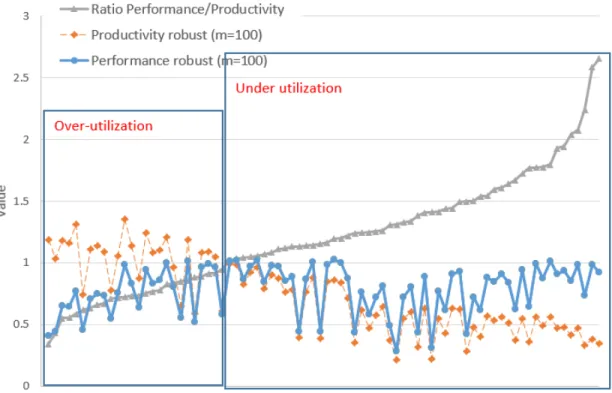
As a further investigation, we present the performance/productivity ratios as a function of the underlying performance and productivity scores. This is visualized in Figure 1. Some interesting patterns emerge. Speci…cally, the schools that are mainly hampered by scarce resources are often super-e¢ cient in terms of the productivity measure. For the given resources, these observations are doing better than expected, which may signal “resource over-utilization”. Those observations would bene…t from weaker resource constraints. By contrast, the schools with unexploited capacity (or “resource under-utilization”) are predominantly those which combine low productivity with high performance. Those observations would bene…t from more stringent resource constraints, because less resources need not impact the output performance.

< Figure 1 about here >

The question remains which are the characteristics of the schools with unexploited capacity (or resource under-utilization) and those which are faced by resource constraints (or resource over-utilization). To address this issue, we estimate the following model:

[

P erfZ_E;m= [P rodZ_E;m= + XE+ E (11)

where denotes a constant, vector with coe¢ cients of the observed characteristics X of observation E, and E an i.i.d. error term. Given the signi…cant di¤erences in under and over-utilization of

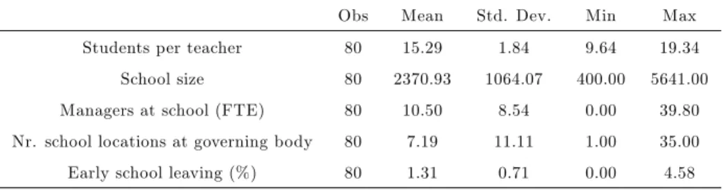
re-sources (see Table 4) we estimate model (11) by a quantile analysis. A standard OLS regression would focus on the conditional mean of the performance/productivity ratio without accounting for its full distributional properties. On the contrary, a quantile regression estimates the potentially di¤erential e¤ect of an independent variable X on various quantiles in the conditional distribution (Koenker and Bassett, 1978). As observed characteristics we include variables which have been indicated in earlier literature (see overview by De Witte and Lopez-Torres, 2017) to in‡uence the productivity and per-formance of schools. They include (1) the number of students per teacher, (2) the school size (number of students in the school), (3) the number of school managers in full time equivalents (FTE), (4) the number of school locations per school district or governing body, and (5) the percentage of early school leavers, de…ned as students who leave the school without higher secondary degree and do not enroll in further education or training. The descriptive statistics are presented in Table 5. They show some signi…cant heterogeneity across the schools. For example, some schools have clearly more students per teachers than other schools. Given the relative autonomy of Dutch schools in spending the lump sum budget, it is intuitive that we observe a negative correlation (-0.14) between the number of students per teacher and the number of managers at a school (expressed in FTE).

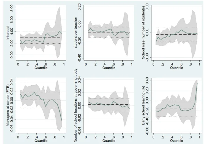
While this regression lacks su¢ cient power to obtain statistically signi…cant outcomes, we do observe some noteworthy patterns. We report in Figure 2 the graphs of the coe¢ cients of the quantile analysis. Each …gure reports for each parameter the complete picture, that is the values each parameter takes, from quantile 0.01 to quantile 1.00. The grey areas denote the 95%-con…dence interval around the estimates.

< Table 5 about here >

< Figure 2 about here >

The negative sign in the …rst graph (student per teacher) suggests that more students per teacher generally corresponds to less unexploited capacity (over-utilization of resources). The estimated cor-relation is roughly similar for all quantiles of the student-teacher ratio. This suggests that the number of students per teacher does vary with having weaker or stronger resource constraints.

Second, smaller schools (in terms of student numbers) are characterized by less unexploited capac-ity, which is not the case for the larger schools. It is interesting to observe that the estimated coe¢ cient slightly increases with the quantile of the number of students at a school. This suggests that larger schools have more unexploited capacity, although the con…dence interval around the estimate also

increases dramatically (due to fewer observations of large schools).

Third, we observe a decreasing pattern for the relationship between the number of school managers (in FTE) and the performance/productivity ratio. For the …rst quantiles of the number of school man-agers, we observe a positive (insigni…cant) correlation to the performance/producativity ratio. This suggests that schools with few managers have a greater degree of unexploited production capacity or technical ine¢ ciency. By moving along the quantiles of the number of school managers the coe¢ cients of the quantile analysis decrease and even become negative. This suggests that for schools with more managers, we can expect more output gains from weaker resource constraints.

Fourth, the number of schools per governing body (school district) does not exhibit a signi…-cant correlation with the performance/productivity ratio. Con…dence intervals are fairly large for all quantiles and, correspondingly, the estimated coe¢ cient is generally close to zero.

Finally, the percentage of early school leavers (school dropouts) correlates negatively and (for some quantiles) signi…cantly to the performance/productivity ratio. These results suggest that early school leaving correlates to resource constraints restricting school performance, which implies that more output gain can be expected from weaker resource constraints. However, while the coe¢ cient is negative for most quantiles of school dropouts, it is positive for the highest quantiles. Although largely insigni…cant, this …nding indicate that schools with a high percentage of early school leavers also have a large degree of unexploited production capacity.

6

Conclusion

Performance of public sector services may be hampered by resource constraints, or may be charac-terized by unexploited capacity. We have presented a novel and simple framework to evaluate the public sector performance in view of these issues. Our method computes performance/productivity ratios, and can be implemented as soon as data on production units’ outcomes and resources are available. Ratio values below unity indicate that better outcomes can be attained through weaker re-source constraints (pointing at scarcity of rere-sources) and, conversely, ratio values above unity indicate that better outcomes can be achieved with the same resources (pointing at unexploited production capacity).

We have demonstrated the practical usefulness of our methodology through an application to secondary schools in the Netherlands. In this application, we also account for outlier behavior and environmental e¤ects by using a robust and conditional nonparametric estimation method. Our em-pirical results indicate that in most cases schools’performance improvement is a matter of unexploited production capacity, while scarcity of resources is a lesser issue. It provides an argument for educa-tional policy makers in times of austerity. While there are schools that do su¤er from stringent resource constraints, the majority of the schools should …rst increase their productivity before requesting ad-ditional funding.

We have also investigated the characteristics of the schools with unexploited capacity and with binding resource constraints. First, we found that under-utilization of resources is positively related to the number of school managers. This …nding is in line with the substantial increase of the number of middle managers in the Netherlands. Due to a consolidation of the number of school districts (i.e.,

more schools per governing body), we could observe an increase in the number of school managers. Our analysis suggests that many schools would bene…t from a reduction of the number of managers. Next, scarcity of resources bears a positive association with the number of students per teacher. This observation provides a hands-on tool for policy makers to analyze the over-utilization of resources. Combing this …nding with the previous one, it can be argued that schools with a high number of students per teacher and a low number of school managers operate under serious resource constraints. Furthermore, larger schools also seem to su¤er from scarce resources. These schools are often located in urban areas, such that they face various challenges due to their unfavorable socioeconomic position. In addition, larger schools typically have a higher complexity, which should be compensated by additional resources. Lastly, resource over-utilization correlates positively to the number of students who leave school without a higher secondary degree and who are not further enrolled in education or training. This suggests that the more early school leavers a school has, the less unexploited capacity there will be. Schools with stringent resource constraints seem to be unable to monitor and prevent early school leaving. Given the substantial societal costs of early school leaving, this suggests that governments should make sure that they provide su¢ ciently large resources to schools to prevent this from happening.

As a concluding remark, while our application in the current paper has focused on education, we emphasize that our methodology can also be relevant in other regulatory contexts. In this respect, a notable example concerns the provision of public services in developing countries. As stated by Estache and Wren-Lewis (2009) “The e¢ cient operation and expansion of infrastructures in developing countries is crucial for growth and poverty reduction”. Mbuvi et al. (2012), for instance, computed simultaneously performance and productivity of water distribution utilities in Africa and showed that there was room for dramatic improvements, near 40%, in both performance and productivity, with the solution relying in most cases on technical ine¢ ciencies rather than on resource constraints.

Appendix 1

As indicated in Section 3, the parameter m in our order-m estimation method serves as a trimming parameter that can tune the percentage of super-e¢ cient DMUs (i.e. DMUs with [P rodE;m > 1 for

our productivity measure and with [P erf_E;m> 1 for our performance measure). We follow Daraio and Simar (2005) to de…ne the value of m. In particular, we systematically increase m and …x it at the value for which the marginal decrease in the fraction of super-e¢ cient DMUs becomes su¢ ciently small. Figure A1 presents the percentage of super-e¢ cient DMUs as a function of m. For low values of m, the percentage of super-e¢ cient observations decreases dramatically, while this percentage decreases at a substantially slower rate when m becomes larger. In our application, we selected m = 100 because the marginal decrease in the fraction of super-e¢ cient observations becomes very small from this point onwards.

References

[1] Afriat, S. (1972). E¢ ciency Estimation of Production Functions. International Economic Review 13, 568-598.

[2] Badin, L., Daraio, C. & Simar, L. (2010). Optimal Bandwidth Selection for Conditional E¢ ciency Measures: A Data-Driven Approach. European Journal of Operational Research 201 (2), 633-640. [3] Banker, R.D., Charnes, R.F. & Cooper,W.W. (1984). Some Models for Estimating Technical and

Scale Ine¢ ciencies in Data Envelopment Analysis. Management Science 30, 1078–1092.

[4] Cazals, C., Florens, J.P. & Simar, L. (2002). Nonparametric frontier estimation: a robust ap-proach. Journal of Econometrics, 106, 1-25

[5] Charnes, A., Cooper, W.W. & Rhodes, E.(1978). Measuring the E¢ ciency of Decision Making Units. European Journal of Operational Research 2, 429–444.

[6] Cherchye, L., Moesen, W., Rogge, N. & Van Puyenbroeck, T. (2007). An introduction to ‘bene…t of the doubt’composite indicators. Social Indicators Research 82, 111-145.

[7] Coelli,T., Estache, A., Perelman, S. & Trujillo, L. (2003). A Primer on E¢ ciency Measurement for Utilities and Transport Regulators. World Bank Institute, Development Studies, The World Bank, Washington, D.C.

[8] Commissie Meijerink. (2008). Over de drempels met taal en rekenen - Hoofdrapport van de expertgroep doorlopende leerlijnen taal en rekenen. Enschede.

[9] Daraio, C. & Simar, L. (2005). Introducing environmental variables in nonparametric Frontier Models: a probabilistic approach. Journal of Productivity Analysis, 24, 93-121

[10] Daraio, C., & Simar, L. (2007). Conditional nonparametric frontier models for convex and non-convex technologies: a unifying approach. Journal of Productivity Analysis, 28 (1-2), 13-32. [11] De Witte, K. and R. Geys (2013), “Citizen coproduction and e¢ cient public good provision:

Theory and evidence from local public libraries”, European Journal of Operational Research, 224, 592-502.

[12] De Witte, K., Geys, B., & Solondz, C. (2014). Public expenditures, educational outcomes and grade in‡ation: Theory and evidence from a policy intervention in the Netherlands. Economics of Education Review, 40, 152-166.

[13] De Witte, K., Haelermans, C. & Rogge, N. (2014). The e¤ectiveness of a computer-assisted math learning program. Journal of Computer Assisted Learning 31 (4), p. 314-329.

[14] De Witte, K, & Lopez-Torres, L. (2017). E¢ ciency in Education. A review of literature and a way forward. Journal of the Operational Research Society, 68 (4), 339-363.

[15] De Witte, K., & Kortelainen, M. (2013). What explains the performance of students in a heteroge-neous environment? Conditional e¢ ciency estimation with continuous and discrete environmental variables. Applied Economics, 45, 2401-2412

[16] Estache, A. & Wren-Lewis, L. (2009). Toward a theory of regulation for developing countries: Following Jean-Jacques La¤ont’s Lead. Journal of Economic Literature, 47 (3), 729-770.

[17] Førsund, F.R. (2017). Measuring e¤ectiveness of production in the public sector. Omega, 93-103. [18] Fried, H.O., Lovell, C.K. & Schmidt, S.S. (Eds.). (2008). The measurement of productive e¢ ciency

and productivity growth. Oxford University Press.

[19] Grifel-Tatjé, E. & Lovell, C.K. (2015). Productivity accounting: the economics of business per-formance: Cambridge University Press.

[20] Hanushek, E. A. (1995). Education production functions. In Durlauf, S. and Blume, L. (Ed.) The New Palgrave Dictionary of Economics, 277-282.

[21] Koenker, R. & Bassett Jr, G. (1978). Regression quantiles. Econometrica 46, 33-50.

[22] Koopmans, T.C. (1951). An analysis of production as an e¢ cient combination of activities. In Activity Analysis of Production and Allocation 33-97. Cowles Commission, Monograph 13 (T.C. Koopmans, ed.), John Wiley and Sons, New York.

[23] Lefebvre, M., Perelman, S. and P. Pestieau (2017), “Productivity and performance in the public sector”, in Grifell-Tatjé, E., Lovell, C. A. K. and R. C. Sickles, Editors, The Oxford Handbook of Productivity Analysis, Oxford University Press.

[24] Li, Q. & Racine, J.S. (2007). Nonparametric Econometrics: Theory and Practice. Princeton University Press.

[25] Lovell, C. K. & Pastor, J. T. (1999). Radial DEA models without inputs or without outputs. European Journal of operational research, 118(1), 46-51.

[26] Lovell, C.A.K, Pastor, J.T. & Turner, J.A. (1995). Measuring Macroeconomic Performance in the OECD: A Comparison of European and Non-European Countries. European Journal of Op-erational Research 87, 507–518.

[27] Mbuvi, D., De Witte, K. & Perelman S. (2012). Urban water sector performance in Africa: A step-wise bias-corrected e¢ ciency and e¤ectiveness analysis. Utilities Policy, 22, 31-40.

[28] Pestieau, P. (2009). Assessing the performance of the public sector. Annals of Public and Coop-erative Economy 80, 133-161.

[29] Varian, H.R.. (1984). The Non-Parametric Approach to Production Analysis. Econometrica 52, 579-598.

T able 1: S ummary sta tistics for in pu ts , outpu ts and con trol v ar iables V a ri a b le n M e a n S .D . M in . 0 .2 5 M e d ia n 0 .7 5 M a x . In p u t v a ri a b le s C o st o f m a te ri a l p e r st u d e n t (e ) 8 0 9 1 4 .9 4 2 5 4 .2 6 4 8 8 .3 7 7 4 6 .1 2 8 8 7 .9 6 1 ,0 3 3 .5 8 1 ,6 7 6 .2 5 C o st o f te a ch e rs p e r st u d e n t (e ) 8 0 6 ,4 3 4 .9 3 9 9 3 .2 2 4 ,8 9 5 .5 4 5 ,9 6 2 .2 4 6 ,3 0 2 .8 4 6 ,7 0 3 .7 1 1 2 ,5 2 3 .5 6 C o st o f h o u si n g p e r st u d e n t (e ) 8 0 5 0 4 .8 9 2 1 2 .8 3 2 5 4 .3 9 3 9 2 .5 2 4 7 4 .6 9 5 5 5 .5 4 1 ,8 6 8 .9 5 T im e d e v o te d to m a th e x e rc is e s (h o u rs ) 8 0 4 5 .3 6 4 0 .1 6 1 .5 1 4 .1 2 9 .9 1 7 8 .6 7 1 7 8 .5 7 O u tp u t v a ri a b le s A v e ra g e sc o re o n th e m a th e x e rc is e s 8 0 1 6 .3 4 1 5 .5 8 0 .8 1 4 .5 9 8 .7 8 2 8 .1 1 6 5 .8 6 A v e ra g e o n th e st a n d a rd iz e d e x a m 8 0 6 .4 5 0 .3 5 .6 6 .3 6 .4 6 .6 5 7 .3 5 C o n tr o l v a ri a b le s % o f st u d e n ts d is a d v a n ta g e d n e ig h b o rh o o d s 8 0 5 .9 5 9 0 0 .1 3 1 .9 8 .0 5 4 1 .8 A v e ra g e a g e o f th e te a ch e rs 8 0 4 5 .0 8 2 .0 9 3 9 .7 4 3 .8 4 5 .0 5 4 6 .3 4 9 .6 A v e ra g e sc o re o f st a n d a rd iz e d e x a m a t e n d o f p ri m a ry e d u c a ti o n 8 0 9 9 .3 8 5 .7 6 8 3 .9 7 9 6 .1 5 9 9 .4 2 1 0 2 .9 5 1 1 7 .6 7

Table 2: Productivity measures Robust Conditional Minimum 0.2172 0.2281 25% 0.4802 0.4998 Average 0.7306 0.7497 St. Deviation 0.2997 0.3157 75% 0.9859 1.0073 Maximum 1.3576 1.7709

Table 3: Performance measures Robust Conditional Minimum 0.2846 0.2850 25% 0.6422 0.6398 Average 0.7825 0.7831 St. Deviation 0.1983 0.1985 75% 0.9486 0.9482 Maximum 1.0260 1.0314

Table 4: Performance/Productivity ratios Robust Conditional Minimum 0.3439 0.3602 25% 0.8535 0.8519 Average 1.2178 1.1897 St. Deviation 0.4701 0.4643 75% 1.4961 1.4402 Maximum 2.6558 2.6630

Table 5: Descriptive statistics of variables which explain the performance/productivity ratio

Obs Mean Std. Dev. Min Max

Students per teacher 80 15.29 1.84 9.64 19.34

School size 80 2370.93 1064.07 400.00 5641.00 Managers at school (FTE) 80 10.50 8.54 0.00 39.80 Nr. school locations at governing body 80 7.19 11.11 1.00 35.00 Early school leaving (%) 80 1.31 0.71 0.00 4.58