Automated rejection and repair of bad trials in MEG/EEG

Automated rejection and repair of bad trials in

MEG/EEG

Mainak Jas, Denis Engemann, Federico Raimondo, Yousra Bekhti, Alexandre

Gramfort

To cite this version:

Mainak Jas, Denis Engemann, Federico Raimondo, Yousra Bekhti, Alexandre Gramfort.

Auto-mated rejection and repair of bad trials in MEG/EEG. 6th International Workshop on Pattern

Recognition in Neuroimaging (PRNI), Jun 2016, Trento, Italy.

HAL Id: hal-01313458

https://hal.archives-ouvertes.fr/hal-01313458

Submitted on 10 May 2016

HAL is a multi-disciplinary open access

archive for the deposit and dissemination of

sci-entific research documents, whether they are

pub-lished or not.

The documents may come from

teaching and research institutions in France or

abroad, or from public or private research centers.

L’archive ouverte pluridisciplinaire HAL, est

destin´

ee au d´

epˆ

ot et `

a la diffusion de documents

scientifiques de niveau recherche, publi´

es ou non,

´

emanant des ´

etablissements d’enseignement et de

recherche fran¸

cais ou ´

etrangers, des laboratoires

publics ou priv´

es.

Automated rejection and repair of bad trials in

MEG/EEG

Mainak Jas

, Denis Engemann

, Federico Raimondo

, Yousra Bekhti

, Alexandre Gramfort

,

1_{CNRS LTCI, T´el´ecom ParisTech, Universit´e Paris-Saclay, France,} 2_{Cognitive Neuroimaging Unit, CEA DSV/I2BM, INSERM, Universit´e Paris-Sud,}

Universit´e Paris-Saclay, NeuroSpin center, 91191 Gif/Yvette, France,

3_{Departamento de Computaci´on, University of Buenos Aires, Argentina}

Abstract—We present an automated solution for detecting bad trials in magneto-/electroencephalography (M/EEG). Bad trials are commonly identified using peak-to-peak rejection thresh-olds that are set manually. This work proposes a solution to determine them automatically using cross-validation. We show that automatically selected rejection thresholds perform at par with manual thresholds, which can save hours of visual data inspection. We then use this automated approach to learn a sensor-specific rejection threshold. Finally, we use this approach to remove trials with finer precision and/or partially repair them using interpolation. We illustrate the performance on three public datasets. The method clearly performs better than a competitive benchmark on a 19-subject Faces dataset.

keywords— magnetoencephalography, electroencephalogra-phy, preprocessing, artifact rejection, automation, machine learn-ing

I. INTRODUCTION

Magneto-/electroencephalography (M/EEG) measure brain activity by recording magnetic/electrical signals in multi-ple sensors. M/EEG data is inherently noisy, which makes it necessary to combine (e.g., by averaging) multiple data segments (or trials). Unfortunately, trials can sometimes be contaminated due to high amplitude artifacts which can reduce the effectiveness of such strategies. Added to this, (the signal in) some sensors can also be bad and repairing or removing them is critical for algorithms downstream in the pipeline. In this paper, we aim to offer an automated solution to this problem of detecting and repairing bad trials/sensors.

Existing software for processing M/EEG data offer a rudi-mentary solution by marking a trial as bad if the peak-to-peak amplitude in any sensor exceeds a certain threshold [1]. The threshold is usually set manually after visual inspection of the data. This can turn tedious for studies involving hundreds of recordings (see the Human Connectome Project [2] as an example of such a large-scale study).

Modern algorithms for rejecting trials compute more ad-vanced trial statistics. FASTER [3], for example, rejects based on a threshold on the z-score of the trial variance, its amplitude range, etc. Riemannian potato filtering [4] works on covari-ances matrices [4] and Artifact Subspace Reconstruction [5] rejects based on the variance of artifact components. However, these methods are not fully satisfactory as rejection thresholds must be fixed or manually tuned. Another promising approach is to apply algorithms robust to outliers. For instance, robust regression [6] can compute an average by downweighting

50

100

150

200

Threshold (

µ

V)

1.8

1.9

2.0

2.1

2.2

2.3

2.4

RM

SE

(

µ

V)

CV scores

auto global

manual

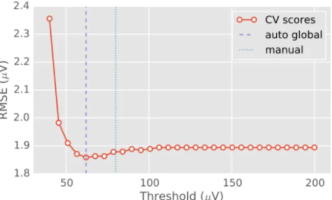
Fig. 1: Mean cross-validation error as a function of peak-to-peak rejection threshold. The root mean squared error (RMSE) between the mean of the training set (after removing the trials marked as bad) and the median of the validation set was used as the cross-validation metric. The optimal data-driven threshold (auto reject, global) with minimum RMSE closely matches the human threshold.

outliers. For single-trial analysis, an outlier detection algorithm is better suited. The Random Sample Consensus (RANSAC) algorithm implemented as part of the PREP pipeline [7], for example, annotates outlier sensors as bad.

In this paper, we make the following contributions. First, we offer a data-driven cross-validation framework (Figure 1) to automatically set the rejection threshold. Secondly, we show that the rejection threshold is sensor-specific and varies considerably across sensors. Finally, we show that taking into account this variation in sensor-specific thresholds can in fact lead to improved detection and repair of bad trials. Our approach unifies rejection of bad trials and repair of bad sensors in a single method.

II. METHODOLOGY

Let us denote the data by X ∈ RN ×P _{where N is the}

number of trials and P is the number of features. P could be QT i.e., the number of sensors Q times the number of time points T if a global threshold has to be computed, or it could be T if only one sensor is considered. To simplify notation, we denote a trial by Xi = (Xi1, Xi2, ..., XiP). Also, we define

the mean of the trials as X = _N1 PN

trials as eX, and the peak-to-peak amplitude of the trials as ptp(Xi) = max(Xi) − min(Xi).

A. Global threshold

If we are estimating an optimal global threshold, then P = QT such that the sensor time-series are concatenated across the second dimension of the data matrix. For a fold k (out of total K folds), the data is split into a training set Xtrainkand a validation set Xvalk such that valk= [1..N ] \ traink (see [8] for another use of cross-validation for parameter estimation in the context of M/EEG). The peak-to-peak amplitudes for all trials Xi in the training set is computed as:

A = {ptp(Xi) | i ∈ traink} (1)

Now, let’s say we have L candidate global thresholds, τl∈ R

for 1 ≤ l ≤ L. Then, for one candidate threshold τl, the set

of indices of the good trials Gl are computed as:

Gl= {i ∈ traink | ptp(Xi) < τl} (2)

The error metric for one fold of the cross-validation for a particular threshold is the Root Mean Squared Error (RMSE) computed as:

ekl= kXGl− eXvalkkFro (3)

where k · k_Fro is the Frobenius norm. The RMSE is computed between the mean of the good trials in the training set Gl

with the median of the trials in the validation set. A low rejection threshold will remove too many trials (leading to high RMSE) whereas a high rejection threshold does not remove the bad trials. Cross validation will find an optimal value which is somewhere in between. The median of the trials in the validation set is used to avoid noisy metric values due to outlier trials. This is inspired from literature on robust cross-validation methods [9], [10] where the loss function is made robust to outlier data.

The threshold with minimum mean error is selected as the global threshold, i.e.,

τ?= τl? with l?= argmin l 1 K K X k=1 ekl . (4)

We call this method auto reject (global). Note that the threshold learnt this way matches values set manually (Fig-ure 1) and is indeed very different across subjects (Fig(Fig-ure 2A). B. Sensor-specific thresholds

In practice however, a global rejection threshold for all sensors is certainly not optimal. Depending on the sensor noise levels and the experiment, each sensor can necessitate a different rejection threshold (Figure 2B). Learning a specific threshold is what we propose next. With a sensor-specific threshold, each sensor votes whether a trial should be marked as good or bad. If a trial is voted as bad by a minimum number of sensors, then it will be marked as bad.

The cross-validation procedure here is the same as in Section II-A except that now P = T . For every sensor, one can thus learn a sensor-specific threshold τ?q where q ∈ [1..Q].

Fig. 2: A. Histogram of thresholds for subjects in the EEGBCI dataset with auto reject (global) B. Histogram of sensor-specific thresholds in gradiometers for the MNE sample dataset (Section III). The threshold does indeed depend on the data (subject and sensor).

However here these thresholds will not be directly used to drop any trial (Equation 5 shows how they are used).

For the cross-validation to work, at least some of the sensor data must be clean. However, this is not the case with globally bad sensors. Therefore, we generate a cleaner copy of each trial by interpolating each sensor from all the others. By doing so, we double the size of the data and generate an augmented matrix Xa ∈ R2N ×T_{. This augmented matrix is}

then used for cross validation (as described in Section II-A). For interpolation, we use the procedure outlined in [11] for MEG and [12] for EEG. Both are implemented in MNE-Python [13] .

Now, let us define an indicator matrix C ∈ {0, 1}N ×Q

whose entries Cij are formed according to the rule:

Cij = ( 0, if ptp(Xij) ≤ τ j ? 1, if ptp(Xij) > τ j ? (5) Each column of this matrix indicates which sensors vote which trials as bad. If the number of sensors which vote a trial as bad exceeds a certain number of sensors κ, then the trial is marked as bad. That is, we take a consensus among the sensors and mark a trial as bad only if the consensus is high enough. In other words, good trials G are given by

G = {i |

Q

X

j=1

Cij < κ} (6)

In practice, we will use κ/Q which is a fraction of the total number of sensors to have a parametrization that is as independent as possible from the total number of sensors. C. Trial-by-trial interpolation

Once we find the bad trials by consensus, the next step is to repair the trials which are good but have a limited number of bad sensors. Since these sensors might be bad locally (i.e., bad for only a few trials) or globally (i.e., bad for all trials), we choose to interpolate the sensors trial-by-trial. Note that we cannot interpolate more than a certain number of sensors. This number depends on the data and the total number of sensors present. Therefore, we choose to interpolate only the worst ρ sensors.

Fig. 3: The evoked response (average of data across trials) on the sample dataset (Section III) for gradiometer sensors before and after applying the auto reject algorithm. Each sensor is a curve on the plots. Manually annotated bad sensor is shown in red. The algorithm finds the bad sensor automatically and repairs it for the relevant trials.

For each trial where the number of bad sensors is larger than ρ, the bad sensors are ranked based on the peak-to-peak amplitude. The higher the peak-to-peak amplitude, the worse is the sensor. That is, we can assign a score sij which is −∞

if the sensor is good and equal to the peak-to-peak amplitude if the sensor is bad.

sij=

(

−∞ if Cij = 0

ptp(Xij) if Cij = 1

(7) This leads us to the following rule for interpolating a sensor Xij: Xij =              interp(Xij), if (0 <P Q j0₌₁Cij0 ≤ ρ) and (Cij= 1) interp(Xij), if (ρ <P Q j0₌₁Cij0 ≤ κ) and (sij > si(N −ρ)) Xij, otherwise (8)

where the notation si(k) indicates the k-th order statistic, i.e.,

the k-th smallest value. interp(·) is a generic function which interpolates the data. That is, when the number of bad sensors in a trial PQ

j=1Cij is less than the maximum number of

sensors ρ which can be interpolated, they are all repaired by interpolation. However, when this is not the case, only the worst ρ sensors are repaired.

The optimal values of parameters κ? and ρ? are estimated

using grid search for the same error metric as defined in Equation 3. We call this method auto reject (local).

III. RESULTS

A. Datasets

We evaluated our algorithms on three publicly available datasets. The first is the MNE sample dataset [13] containing

0.5

1.0

1.5

2.0

2.5

no reject RM

SE

(

µ

V)

0.5

1.0

1.5

2.0

2.5

auto reject RMSE (

µ

V)

0.5

1.0

1.5

2.0

2.5

RANSAC RM

SE

(

µ

V)

Fig. 4: RMSE with no rejection applied, auto reject (global), and RANSAC. Each point represents a subject from the Faces dataset [15]. Auto reject has a better RMSE whenever a point lies above the dotted red line. Note that auto reject almost always performs as well as or better than the other methods.

204 gradiometer sensors (1 globally bad) and 102 magnetome-ter sensors. The second is the EEGBCI motor dataset [14] with 104 subjects and the final one is the Faces dataset [15] with 19 subjects. The bad channel annotations for each run and subject was available from the authors of the Faces dataset [15].

For the EEGBCI and MNE sample dataset, the trials are 700 ms long with a baseline period of 200 ms with respect to the trigger (auditory left tone for MNE sample and resting for EEGBCI). In the Faces dataset, we use the trials where famous faces were shown. The data was bandpass filtered between 1 and 40 Hz. The trials were 1 s long with a baseline period of 200 ms.

B. Auto reject (global)

Figure 1 shows, on the sample dataset, how the global threshold can be selected by cross-validation. One can observe how a low rejection threshold leads to high RMSE due to removal of too many trials whereas high rejection threshold leads to high RMSE because the bad trials are not removed. The reader may note that the automatic threshold is very close to a carefully chosen manual threshold. Figure 2A shows the results computed for 104 subjects in the EEGBCI dataset. Note that the threshold does indeed vary across subjects.

C. Auto reject (local)

This auto reject (local) approach finds the thresholds at the level of each sensor. The candidate thresholds used vary be-tween 2–400 µV for EEG; 400–20000 fT/cm for gradiometers; and 400–20000 fT for magnetometers.

Figure 2B demonstrates that the sensor-level thresholds for rejection are indeed different across sensors. This is the moti-vation for the more fine-grained technique based on consensus. Figure 3 demonstrates that the algorithm indeed improves the data quality. The bad MEG sensor which showed high

fluctuations before applying the algorithm is repaired after application of the algorithm.

We compared our proposed algorithm to the RANSAC implementation in the PREP pipeline [7]. RANSAC being an algorithm robust to outliers, serves as a competitive bench-mark. To generate the ground truth for comparison, 4/5ths of the available trials were averaged and the bad channels interpolated per run. Outliers will have negligible effect in the ground-truth as it is obtained by averaging a large number of trials. It is this ground-truth which is used for computing the RMSE. This is a nested cross-validation setting where the validation set used for optimizing the thresholds is different from the ground truth (test set). The bad sensors detected by RANSAC (with default parameters) were interpolated before comparison to the ground truth. Figure 4 shows that auto reject (local) indeed does better than not rejecting trials or applying RANSAC. Of course, if annotations of bad sensors per epochs were available, auto reject will have an even better score because of how it works. We found that RANSAC results depend greatly on the input parameters (results omitted due to space constraints) which is probably why it does not perform as well as auto reject.

IV. DISCUSSION

The algorithm described here is fully automated requiring no manual intervention. This is particularly useful for large-scale experiments. It also implies that the analysis pipeline is free from experimenter’s bias while rejecting trials.

A big strength of the auto reject algorithm is that the average evoked response obtained can be used in noise-normalized source modeling techniques such as dSPM or sLORETA without any modifications. Indeed, such methods are not readily applicable if the average is a weighted mean (as in robust regression [6]), which changes how the variance of the noise should be calculated. However this is not the case in our method.

Compared to other methods (e.g., PREP [7]), we do not make the assumption that sensors must be globally bad. In fact, it can detect and repair sensors even when they are locally bad, thus saving data. Of course, with suitable modifications, the method can also be used to detect flat sensors. Note that, even though we used peak-to-peak threshold as our statistic for trials, our algorithm should work with other reasonable statistics too.

To avoid the dangers of double dipping, our advice is to run the algorithm on each condition separately and not on the contrast. Instead of using spline interpolation or Minimum Norm Estimates to clean the sensor data in Section II-B, one could also use the SNS algorithm [16] or the algorithm based on Signal Space Separation [17]. Our algorithm is complemen-tary to these efforts and can only benefit from improvements in these techniques. Comparing these interpolation methods and their effect on our algorithm will be done in future work. Finally, when spatial filtering methods [18], [19] are used for artifact removal, they should be applied after our algorithm.

V. CONCLUSION

We have presented an algorithm to automatically reject and repair bad trials/sensors based on their peak-to-peak amplitude which is so far done manually in standard preprocessing pipelines. The algorithm was tested on three publicly available datasets and compared to a competitive benchmark. Finally, the code will be made publicly available.

VI. ACKNOWLEDGEMENT

This work was supported by the ANR THALAMEEG, ANR-14-NEUC-0002-01 and the R01 MH106174.

REFERENCES

[1] A. Gramfort, M. Luessi, E. Larson, D. Engemann, D. Strohmeier et al., “MNE software for processing MEG and EEG data,” NeuroImage, vol. 86, no. 0, pp. 446 – 460, 2014.

[2] D. Van Essen, K. Ugurbil, E. Auerbach, D. Barch, T. Behrens, R. Bu-cholz, A. Chang, L. Chen, M. Corbetta, S. Curtiss et al., “The Hu-man Connectome Project: a data acquisition perspective,” NeuroImage, vol. 62, no. 4, pp. 2222–2231, 2012.

[3] H. Nolan, R. Whelan, and R. Reilly, “FASTER: fully automated statis-tical thresholding for EEG artifact rejection,” J. Neurosci. Methods, vol. 192, no. 1, pp. 152–162, 2010.

[4] A. Barachant, A. Andreev, and M. Congedo, “The Riemannian Potato: an automatic and adaptive artifact detection method for online experiments using Riemannian geometry,” in TOBI Workshop lV, 2013, pp. 19–20. [5] C. Kothe and T. Jung, “Artifact removal techniques with

signal reconstruction,” Jul. 16 2015, wO Patent App. PCT/US2014/040,770. [Online]. Available: http://www.google.com/ patents/WO2015047462A9?cl=en

[6] J. Diedrichsen and R. Shadmehr, “Detecting and adjusting for artifacts in fMRI time series data,” NeuroImage, vol. 27, no. 3, pp. 624–634, 2005.

[7] N. Bigdely-Shamlo, T. Mullen, C. Kothe, K.-M. Su, and K. Robbins, “The PREP pipeline: standardized preprocessing for large-scale EEG analysis,” Front. Neuroinform., vol. 9, 2015.

[8] D. Engemann and A. Gramfort, “Automated model selection in co-variance estimation and spatial whitening of MEG and EEG signals,” NeuroImage, vol. 108, pp. 328–342, 2015.

[9] D. Leung, “Cross-validation in nonparametric regression with outliers,” Ann. Stat., pp. 2291–2310, 2005.

[10] J. De Brabanter, K. Pelckmans, J. Suykens, J. Vandewalle, and B. De Moor, “Robust cross-validation score functions with application to weighted least squares support vector machine function estimation,” K.U. Leuven, Tech. Rep., 2003.

[11] M. H¨am¨al¨ainen and R. Ilmoniemi, “Interpreting magnetic fields of the brain: minimum norm estimates,” Med. Biol. Eng. Comput., vol. 32, no. 1, pp. 35–42, 1994.

[12] F. Perrin, J. Pernier, O. Bertrand, and J. Echallier, “Spherical splines for scalp potential and current density mapping,” Electroen. Clin. Neuro., vol. 72, no. 2, pp. 184–187, 1989.

[13] A. Gramfort, M. Luessi, E. Larson, D. Engemann, D. Strohmeier et al., “MEG and EEG data analysis with MNE-Python,” Front. Neurosci., vol. 7, 2013.

[14] A. Goldberger, L. Amaral, L. Glass, J. Hausdorff, P. Ivanov et al., “Physiobank, physiotoolkit, and physionet components of a new research resource for complex physiologic signals,” Circulation, vol. 101, no. 23, pp. e215–e220, 2000.

[15] D. Wakeman and R. Henson, “A multi-subject, multi-modal human neuroimaging dataset,” Sci. Data, vol. 2, 2015.

[16] A. De Cheveign´e and J. Simon, “Sensor noise suppression,” J. of Neurosci. Methods, vol. 168, no. 1, pp. 195–202, 2008.

[17] S. Taulu, J. Simola, M. Kajola, L. Helle, A. Ahonen et al., “Suppression of uncorrelated sensor noise and artifacts in multichannel MEG data,” in 18th international conference on biomagnetism, 2012, p. 285. [18] R. Vig´ario, “Extraction of ocular artefacts from EEG using independent

component analysis,” Electroen. Clin. Neuro., vol. 103, no. 3, pp. 395– 404, 1997.

[19] M. Uusitalo and R. Ilmoniemi, “Signal-space projection method for separating MEG or EEG into components,” Med. Biol. Eng. Comput., vol. 35, no. 2, pp. 135–140, 1997.