PROCEEDINGS OF SPIE
SPIEDigitalLibrary.org/conference-proceedings-of-spie
The Talbot effect's impact on the high
contrast imaging modes of METIS
Boné, André, Agócs, Tibor, Absil, Olivier, Delacroix,
Christian, Amorim, António, et al.
André Boné, Tibor Agócs, Olivier Absil, Christian Delacroix, António Amorim,
Jeff Lynn, "The Talbot effect's impact on the high contrast imaging modes of
METIS," Proc. SPIE 11451, Advances in Optical and Mechanical Technologies
The Talbot effect’s impact on the high contrast imaging
modes of METIS
André Boné
a,b, Tibor Agócs
b, Olivier Absil
c, Christian Delacroix
c, António Amorim
a, and Jeff
Lynn
ba
Faculty of Sciences University of Lisbon, Lisbon, Portugal
b
NOVA Optical IR Instrumentation Group, ASTRON, Dwingeloo, The Netherlands
cUniversité de Liège, Liège, Belgium
ABSTRACT
The ELT, Europe’s Extremely Large Telescope, with its 39m main mirror will be the largest optical/infrared telescope in the world, able to work at the diffraction limit. METIS is one of its first light instruments with powerful imaging and spectroscopic capabilities in the thermal wavelengths. It contains several high contrast imaging (HCI) modes, which allow it to detect and characterize exoplanets amongst others. The HCI performance is highly dependent on pupil stabilization mechanisms and a closed loop compensation of non-common path aberrations degrading the wavefront error of the instrument.
The Talbot effect is a near-field effect on collimated light, where spatial frequencies of the wavefront are re-imaged periodically along the optical path. The periodicity is known as the Talbot length, which is a function of the wavelength and the wavefront’s spatial frequencies with the latter being a result of the wavefront errors caused by the surface form errors of optical elements. The aberrations oscillate from amplitude to phase, in the spatial scale of one Talbot length, which can have an impact on the performance of the HCI modes. We evaluate the impact of the Talbot effect with respect to the METIS phase aberration budget by assuming representative power spectral density profile for the surface form error of each optical surface. We propagate the errors to the subsequent pupil plane and finally investigate the resulting point spread function profile. Simulations are fed back into the HCI error budget and if necessary, the specifications regarding instrument surface form are adjusted.
Keywords: Optics, HCI, ELT, METIS, Talbot effect, Fourier propagation
1. INTRODUCTION
The Mid-infrared ELT imager and spectrograph, or METIS for short, is one of the first generation scientific instruments of the extremely large telescope (ELT), and the only one to focus on the thermal infrared. METIS will provide imaging at 3 to 13 µm, over a field of view (FOV) of approximately 11′′× 11′′, and integral field
spectroscopy at 3-5 µm (instantaneous spectral range of≈ 50 nm) with high resolution (R ≈ 105), over a FOV
of approximately 1′′× 0.5′′. All its observing modes work at the diffraction limit of the ELT, with a single
conjugate adaptive optics (SCAO) module which yields an angular resolution of 0.023′′ at 3.5 µm. METIS will have a spatial resolution six times better than the mid-infrared instrument on the James Webb space telescope (JWST), and, at the mid-infrared range, it will exceed the Hubble Space Telescope’s resolution at optical wavelengths. Furthermore, its spectral resolution is 30× higher than the one of the mid-infrared instrument on
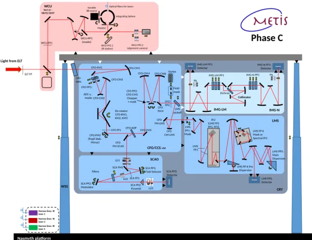
the JWST.1The METIS optical schematics is shown inFigure 1.
METIS contains several subsystems, each responsible for an essential part of the METIS’ functions. These are: the cryostat (CRY), the common fore optics (CFO), the imager (IMG), the L/M Spectrograph (LMS), the single-conjugate adaptive optics module (SCA or SCAO), the warm calibration unit (WCU), and the warm support structure (WSS).
Further author information: (Send correspondence to André Boné) André Boné: E-mail: [email protected]
CFO/CCS v9d CFO PP1: ADC-s, masks CRY-WIN CFO-AOP De-rotator CFO-KM1, KM2, KM3 CFO FP1 CFO PP2: CFO-CM5 Chopper + mask CFO FP2 CFO-CM1 CFO-CM2 CFO-CM3 CFO-FM2 (Pupil Stab. Mirror) CFO-FM3 CFO-CM4 CFO-CM6 CRY LMS pickoff CFO-FM1 CFO FM-SCAO Nasmyth platform
Light from ELT
Integrating Sphere Mask(s) WCU-FP2.2 (alignment camera) Variable BB source WCU-FP2.1 (IR station) CCD WCU-PP1 (masks) WCU Ver1.0 – 08/01/2019 WCU-FP1 Field-mask Vortex Dichroic Collimator IMG-LM IMG-LM PP1 PIL IMG-N FP1: Detector IMG-N PP1 IMG-N PIL IMG-LM FP1: Detector SCA PP1: Field Selector LU1 LU2 SCA PP2: Modulator Filters SCA FP2: Pyramid SCA PP3: Detector LU3 SCA FP1 SCAO WSS CFO FM4 CFO FM-LMS CFO CM-LMS LMS PP5: Main Dispersion LMS FP5: Detector LMS PP4: Pre Dispersion LMS LMS PP1: Mask LMS FP4: Mask or Spectral IFU IFU (LMS FP2 PP3, FP3) LMS FP1 ELT FP
Phase C
SCA FM1 Optical fibers for lasersNarrow lines IR laser 1 Narrow lines IR laser 2 Narrow lines IR laser 3
Figure 1: Optical diagram overview of METIS. The different background colors represent different temperature zones.2
In order to decrease the thermal background and the number of warm surfaces, most of METIS’ optics are inside a cooled cryostat. The exception is the WCU, which is the subsystem that provides optical sources used to monitor, troubleshoot, and calibrate the response of METIS in all observing modes. The WSS is also outside the CRY, but it is only a support subsystem which does not contain optics of its own.
The light enters the CFO, which is at the core of the CRY. It provides chopping, image de-rotation or pupil co-rotation, pupil stabilisation, and stray light and thermal background reduction. All this is crucial for optimised operation and good science performance needed for METIS. It also provides optical interfaces with the IMG, the LMS, the SCA and WCU subsystems. The CFO also provides mechanical and thermal interfaces to the other cold subsystems.2
The LMS is the sub-system that provides high spectral resolution (R = 105 at 4.65 µm) integral field
spec-troscopy. A dichroic acts as a beam splitter, guiding the light into the LMS. This dichroic is retracted for imaging the L/M and N bands in the imager. Inside the LMS, a selection of pupil masks and coronographic elements for high contrast imaging (HCI) are available at the LMS PP1. The integral field unit will then stack the spatial samples along one dimension. Afterwards, the beam is dispersed and re-imaged onto the detector’s focal plane. The integral field unit (IFU) also includes coronagraphy for high contrast spectroscopy, and a mode which provides instantaneous ≈ 5-fold increase in spectral range.2
The IMG provides diffraction limited imaging from 2.9 to 13 µm, as well as coronagraphy and long-slit spec-troscopy. A dichroic mirror splits the light into two channels, one for the L/M band and the other for the N band,
for optimal performance. The cameras offer several spectral filters for direct imaging and a set of coronagraphic masks for HCI.
A vortex phase mask can be placed at the focal plane CFO FP2, before both the LMS and IMG.
METIS is currently on phase C. However, one of the questions raised during the preliminary design review of METIS was if the Talbot effect would influence the high contrast imaging (HCI) modes of METIS by introducing unexpected amplitude aberrations. To answer that question, we modelled this effect on the optics of METIS through wave propagation.
2. THE TALBOT EFFECT
The Talbot effect is a consequence of the wave behaviour of light. This effect, first discovered by Henry Talbot in 1836,3 is a near-field effect on collimated light that reimages a grating periodically along the optical path.
The period of this reimaging is known as the Talbot length (LT), and it is a function of the spatial period of the
grating Λ and the wavelength λ, given by
LT=
2Λ2
λ . (1)
This effect is a consequence of the free-space propagation. For instance, let’s consider a grating with a sinusoidal transmission at z = 0, which, when illuminated by a uniform light source, creates a field given by
u0(x) = 1 + a sin ( 2πx Λ ) , (2)
where a is the magnitude of the amplitude variation. The propagated field at a distance z is given by the Fourier formalism. For this we use the free-space transfer function4,5
Hz(ξ) = ej
2πz
λ e−jπzλξ
2
, (3)
where ξ represents the spatial frequencies in the x direction, and j is the imaginary unit. This function used the Fresnel approximation for the near field, but it is also valid if the grating period is larger than the wavelength5
(the opposite of a diffraction grid). By using Hz(ξ) to propagate the field u(x), we get uz(x) = u0(x)∗ F−1[Hz(ξ)] = ej 2πz λ [ 1 + a sin ( 2πx Λ ) e−j2πLTz ] . (4)
By ignoring the piston phase term ej2πz
λ , and rewriting the complex field in the form of
uz(x) = Az(x) exp[jΨz(x)], where Az(x) is the amplitude, and Ψz(x) is the phase, we obtain
Az(x) = √ 1 + 2a sin ( 2πx Λ ) cos ( 2π z LT ) + a2sin2 ( 2πx Λ ) ≈ 1 + a sin ( 2πx Λ ) cos ( 2π z LT ) (5) and Ψz(x) = arctan −a sin(2πx Λ ) sin ( 2πLz T ) 1 + a sin(2πxΛ )cos ( 2πLz T ) ≈ −a sin ( 2πx Λ ) sin ( 2π z LT ) . (6)
These approximations are obtained by assuming that a≪ 1, i.e. that it represents a small perturbation. From
there the amplitude and the phase are approximated to the linear terms of their Taylor series in a.5
These equations show that a small initial periodic perturbation will oscillate between phase and amplitude along the optical axis, with a period given by the Talbot length. In this case, a small amplitude variation induced the effect, but by applying a variable substitution given by z = z′−LT
4 these equations become
Az′(x)≈ 1 + a sin ( 2πx Λ ) sin ( 2π z ′ LT ) (7)
and Ψz′(x)≈ a sin ( 2πx Λ ) cos ( 2π z ′ LT ) . (8)
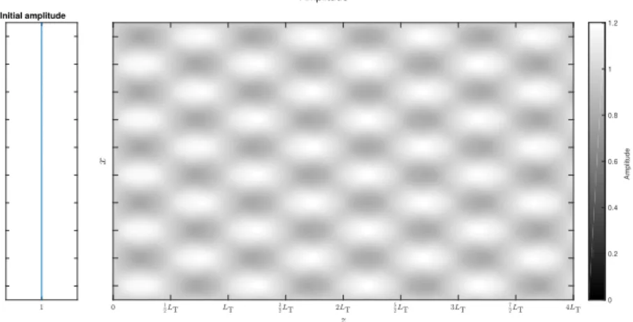
The equations are equivalent, but they show that, at z = 0, there is no amplitude aberration, but only phase aberrations. This indicates that an initial phase aberration also induces the Talbot effect, which is shown in the simulation ofFigure 2. Initial amplitude Amplitude 0 0.2 0.4 0.6 0.8 1 1.2 Amplitude
(a) Amplitude pattern due to the Talbot effect. Initial amplitude is uniform.
Phase (radians) Initial phase Phase -0.2 -0.15 -0.1 -0.05 0 0.05 0.1 0.15 0.2 Phase (radians)
(b) Phase pattern due to the Talbot effect. Initial amplitude is uniform.
Figure 2: Simulation, using the Fourier formalism for wave propagation, showing the effects of an initial small phase variation on the phase and amplitude along the optical path (z) due to the Talbot effect.
In the case of METIS, the surface form error (SFE) of the optical surfaces can induce small perturbations on the phase. These perturbations can lead to unexpected impacts on the amplitude of the wavefront, affecting the HCI modes. It is necessary to look at the propagation of light using the Fourier formalism on the optics of METIS. Unfortunately, the design and analysis of METIS is mostly done on ZEMAX®, which is a powerful ray-tracing software, but is not our tool of choice for the wavefront analysis. We developed a Python script which imports the optical geometry using ZEMAX®’s API (ZOSAPI), and uses the PROPER library6 for Python to
propagate the wavefront.
The Talbot effect is described in the collimated space, so our script calculates the conjugated plane in the collimated space for every surface. The propagtion is then done on this collimated space, from the entrance pupil of METIS to the first pupil of the LMS or the IMG, where the Lyot stops and apodizing phase plates are placed.
2.1 Determining the distance position on the collimated space.
The surface properties and their locations are imported from ZEMAX® using its API (ZOSAPI), which allows the user to run ZEMAX® features and analyses from a script. The system aperture, fields, and wavelengths are all imported into the script as well.
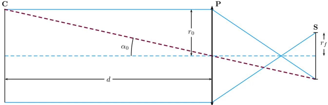
One of the approximations of the script is to ignore the curvature of the surfaces, and treat them as planes. In other words, each surface is treated as a paraxial lens which is a plane that changes the rays’ trajectories as would a lens or a mirror. The chief ray for the central field defines the centre of each surface plane. The position the ray hits each surface is given by the single ray simulation. The next step is to calculate the conjugated plane in the collimated space, for which we developed a simple geometrical method, exemplified inFigure 3.
P S C α0 r0 d rf
Figure 3: Using chief rays to calculate the conjugated plane C of surface S. The pupil plane P has a radius of aperture r0, and the surface S has a footprint radius rf. The conjugated plane of the surface S is the plane C,
which is at a distance d from the pupil. The blue thin rays (dashed line is the chief ray, and full lines are the marginal rays) represent the central field, while the red thick dashed ray is the chief ray of a field with an angle
α0. This angle is such that the chief ray hits the surface S at a distance rf from the centre, and passes through
the plane C at a distance r0 from the centre.
If a chief ray from a deviated field hits the surface on the border of its footprint, then the same should happen on the conjugated plane. Since the footprint radius on the collimated space is the same as the optical aperture radius r0, and, as a chief ray, it hits the centre of the entrance pupil, then the distance d between the conjugated
plane and the pupil is given by
d =± r0
tan α0
, (9)
where α0 is the field’s angle. Translating this into normalized coordinates, we get α0 = h0αmax, where αmax
is the largest field angle, which is known, and h0 corresponds to the absolute value of the field in normalized
coordinates. What remains is to find the value of h0. This is done by sending a random chief ray and check
the distance r from where it hits the surface to its centre. It is easy to see that r∝ tan hαmax, where h is the
absolute value of the field of the ray in normalized coordinates. Applying a three simple rule and going back to equation (9) leads to d =±r0 rf r tan hαmax , (10)
where rf is the footprint radius, calculated beforehand by using marginal rays for the central field, and average
the distances of their hit position to the centre of the surface.
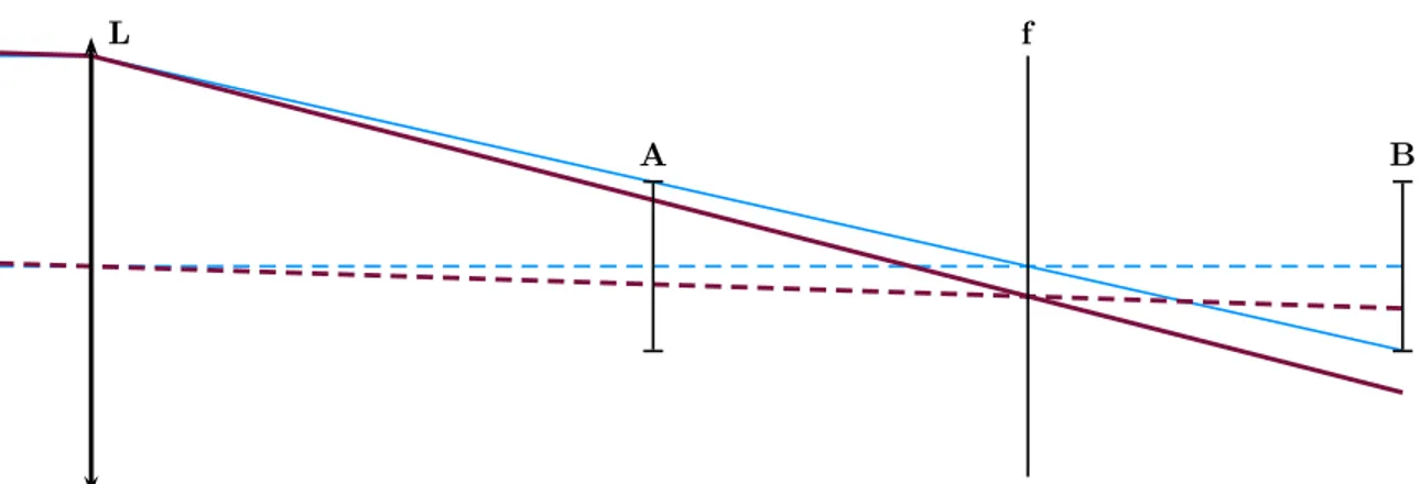
This procedure is repeated several times for different random chief rays in order to have a statistic sample and evaluate the repeatability of this method. However, this method does not distinguish between upstream or downstream conjugated planes, and all values of d are positive. It is, therefore, necessary to calculate the correct sign, since it is crucial to know the direction the wavefront will be propagated. For this, we developed another geometrical method, represented inFigure 4.
L f
A B
Figure 4: Marginal rays hitting surfaces A and B, located before and after a focal plane respectively. The lens
L creates a focus plane f between surfaces A and B. The chief rays are represented by dashed lines, and the
marginal rays by full lines. The central field is represented by blue thin lines, and the small angle field by red thick lines. The footprints of the surfaces are determined by the marginal ray of the central field. The marginal ray from the small angle field hits surface A within its footprint area, but hits surface B outside it.
From the lens equation, if a surface is after a focal plane, the conjugated plane is before the pupil. If the surface is before a focal plane, the conjugated plane is after the pupil. So, in order to determine the sign of d, we need to check the surface’s relative position to a focal plane. The method shown inFigure 4uses marginal rays of small fields and checks the distance r from where they hit the surface to its centre. If r < rf, then the
surface is before a focal plane, otherwise it is after a focal plane.
The results from this method were tested manually in ZEMAX® by applying a point source on the calculated conjugated position, and checking whether or not a focal plane would form at the surface’s position. This check was useful to show that the methods were working correctly, and it even showed that the method to define the sign of d is only valid if the field angle is small enough. It is easy to understand why, as it is possible to imagine, fromFigure 4, a field whose marginal ray would cross the chief ray of the central field and eventually hit surface
A outside the footprint radius.
3. PROPAGATION
Propagation is done using the Fourier formalism (angular spectrum and Fresnel), through the PROPER libraries for Python,6which contain all the necessary functions pre-built. The PROPER library chooses the best algorithm
automatically, using the method described in.7
The light starts at the entrance pupil as a plane wavefront with uniform amplitude and phase, where a circular aperture with a circular central obscuration is implemented. The aperture and obscuration represent the ELT’s aperture and M2 obscuration, on a grid with size 1024× 1024 pixels. A black border is then applied
in order to oversize the grid to 2.5× the aperture diameter and avoid unwanted vignetting and numerical issues,
as explained before. In other words, the simulation will work with a full grid of 2560× 2560 pixels.
The light is then propagated from between the conjugated planes, as will be described onsection 3.1. Each conjugated plane adds its corresponding phase error (given by the surface form error). The process of generating randomized SFE and propagating is repeated 50 times in order to get statistically representative results. However, running this script takes a very long time. For a sampling of 1024× 1024 pixels, running the analysis for the
CFO, up to the LMS and the IMG, takes a few days.
3.1 How to correctly propagate the wavefront on the collimated space
The light is propagated from the pupil to the conjugated plane of the first surface, where the first phase aber-rations are introduced. Then it is propagated to the conjugated plane of the second surface, and so on until it
reaches the last surface. Then it is again propagated to the pupil. Some surfaces do not add phase errors but apply masks, which can cause diffraction effects.
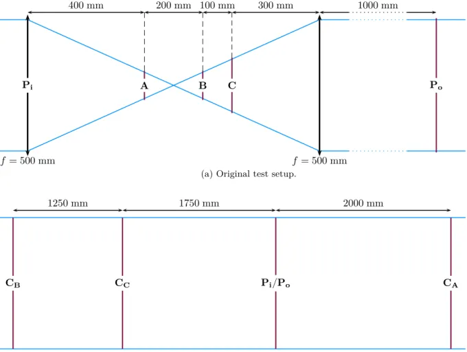
The reason propagation is done like this is because it has shown to give more realistic results. In fact, we analysed three methods to make the propagation. For this analysis, we developed the simple test setup of
Figure 5.
Pi A B C Po
f = 500 mm f = 500 mm
400 mm 200 mm 100 mm 300 mm 1000 mm
(a) Original test setup.
Pi/Po CA
CB CC
1250 mm 1750 mm 2000 mm
(b) Collimated space of test setup.
Figure 5: Setup for testing wavefront propagation methods. A lens of focal length 500 mm is placed at the entrance pupil Pi. Surfaces A, B, and C introduce phase aberrations, and the light is then propagated through
another lens until the exit pupil Po. The results are compared with the propagation made through the conjugated
planes CA, CB, and CCin the collimated space.
This test setup consists of two lenses of focal length f = 500 mm. The first lens is placed at the entrance pupil Pi, and the second is placed 1000 mm downstream in order to create a relay. This places the exit pupil Po
1000 mm after the second lens.
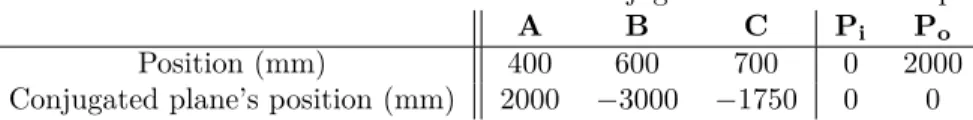
In between the lenses, there are three surfaces that introduce phase aberrations. Surfaces A and B are placed on each side of the focal plane, at the same distance from it. Surface C is placed after surface B. Their absolute positions and the corresponding conjugated planes in the collimated space are on Table 1.
The phase error ∆ϕs introduced by the surface s, is given, in radians, by
∆ϕA= 0.2π sin [50π(x + y)] ∆ϕB= 0.2π sin [50πx] ∆ϕC= 0.2π sin [25πy] , (11)
Table 1: Positions of the surfaces and their conjugates for the test setup.
A B C Pi Po
Position (mm) 400 600 700 0 2000
Conjugated plane’s position (mm) 2000 −3000 −1750 0 0
where x and y are the coordinates on the plane, and the footprint radius is√x2+ y2= 0.3 mm. These dimensions
are for the collimated space.
The wavelength used is λ = 1 µm. First, the light is propagated on the test setup using Fourier formalism. The system considers an aperture with a radius of 0.3 mm, and then applies to it a phase curvature
∆ϕL = 2π λf √ 1 + x 2+ y2 f2 , (12)
which corresponds to the lens focal distance. Surfaces A, B, and C are rescaled appropriately to fit the footprint. Furthermore, surface A is also mirrored in x and y because it is placed before the focal point. After reaching each surface, the corresponding phase error is applied, as well as a vignetting mask with the surface’s radius. This guarantees that some diffraction effects will be present. The light is then propagated to the next surface. When it reaches the second lens, the phase curvature ∆ϕL is again applied, but no vignetting mask, since that
would require an extra mask on the collimated space. The light is finally propagated to the exit pupil, where the last vignetting mask, with a radius of 0.3 mm is applied. The results of this propagation are inFigure 6. The tests consist of trying to replicate these results using only the surfaces on the collimated space.
−1.00 −0.75 −0.50 −0.25 0.00 0.25 0.50 0.75 1.00 −1.00 −0.75 −0.50 −0.25 0.00 0.25 0.50 0.75 1.00
Original Amplitude
0.0 0.5 1.0 1.5 2.0 2.5(a) Amplitude retrieved using the original test setup.
−1.00 −0.75 −0.50 −0.25 0.00 0.25 0.50 0.75 1.00 −1.00 −0.75 −0.50 −0.25 0.00 0.25 0.50 0.75 1.00 Original Phase −2.0 −1.5 −1.0 −0.5 0.0 0.5 1.0 1.5
(b) Phase retrieved using the original test setup.
Figure 6: Results of the propagation simulation using the original test setup.
The first method to be tested consisted in propagating the phase aberrations of each surface to the pupil, and average them. However, since propagation is a non-linear operation, this method failed to replicate the data. The phase difference between the original phase and the one obtained through this method presented a standard deviation (inside the footprint) of 0.5052 radians.
The second method was based on an algorithm used in adaptive optics8that consists in multiplying the
then multiplying the complex amplitudes. But since the amplitude is being multiplied it loses physical meaning. The phase, however, got closer to the original one. The difference between them presented a standard deviation (inside the footprint) of 0.2043 radians.
Finally the third method consisted in propagating the wavefront from the pupil to CA, then from CA to
CB, then to CC, and finally again to the pupil. This method is intrinsically serial and is not easily parallelized,
unlike the other two∗.
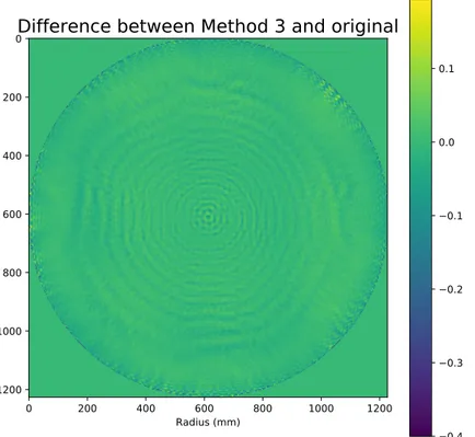
Both the amplitude and phase were replicated almost perfectly. It is worth noticing that a perfect replication is not expected due to numerical limitations since the surfaces have different samplings than their conjugates due to their reduced footprint diameter. The difference between the original phase and the one obtained was computed again. It is shown inFigure 7. It presents a standard deviation (inside the footprint) of 0.0019 radians, which is much smaller than the other two methods, and inFigure 7 we can see that phase differences seem to occur only due to a small deviation in diffraction lines.
0 200 400 600 800 1000 1200 Radius (mm) 0 200 400 600 800 1000 1200 Ph a e (r ad ian )
Difference between Method 3 and original
−0.4 −0.3 −0.2 −0.1 0.0 0.1
RMS: 0.019 radian
Figure 7: Difference between the original phase and the one obtained through the third method. With this we concluded that this third method was indeed capable of replicating the wavefront error of a system using only the collimated space.
4. GENERATING A RANDOMIZED SURFACE FORM ERROR
The imperfections of the optical surfaces introduce the spatial frequencies that are reimaged by the Talbot effect. In order to run a good analysis, it is necessary to create realistic SFE for each surface. Depending on the impact of the Talbot effect, the budget for the quality of the optical elements might need to be revised, and new specifications for the surfaces’ form errors defined.
∗For the first two methods, the parallelization consisted of having different threads propagating different surfaces to the
pupil. However, since the propagation would run several times for different SFE, the parallelization of the third method consisted of running the propagation with different SFE for each thread.
The SFE were generated according to the description of Agócs.9 Random Zernike polynomials are used to
model the low and mid spatial frequency components. These can be caused by surface manufacturing, print-through errors, and other low order contributors such as mechanical mounting stresses and errors, thermal gradients, and gravitational sagging.9 Mid and high spatial frequencies can also be caused by print-through
and manufacturing errors, and they are modelled with PSD functions. All errors are defined over the footprint corresponding to the central field position.
Higher spatial frequencies on the surface shape, whether modelled through higher order Zernike polynomials or by the PSD, contribute much more to the final WFE than lower frequencies. It was noted that, in order to have a realistic representation of a surface, the lower frequency Zernikes and the higher frequency PSD errors could not have the same weight. For this reason, the surface form error is represented by three contributors: 1. a random Zernike polynomial (ZA) between the 2nd and the 20th term (using the OSA notation); 2. a random
Zernike polynomial (ZB) between the 21stand the 54thterm†; 3. an inverse power law 1D PSD function.10 The
total surface RMS is then budgeted into these three contributors, each with half of the weight of the previous one. In other words, for a total surface RMS of σ0 separated into the three contributors σZA, σZB, σPSD, we get
that { σ2 0= σZA2 + σ2ZB+ σPSD2 σZA= 2σZB= 4σPSD ⇔ { σZA= σ0 √ 16 21 σPSD= σZB2 =σZA4 . (13)
This is an empirical method based on personal and practical experience inside the METIS group and has been deemed to be realistic.
The Fourier spectrum of the height map of an optical surface provides the surface’s PSD. It is commonly used to characterize mid and high-spatial frequency height errors and specify a surface’s quality. However, the inverse is also possible, and by admitting a particular shape for this function, one can generate a synthetic random height map for a surface. In this work, we presume that the PSD can be represented by a 1D inverse power law10 given by PSD = σ 2 PSDA h0 1 1 + ( ρ ρc )P, (14)
where A is the surface’s area, ρ represents the spatial frequencies given in polar coordinates, ρc is the cutoff
frequency (or half power frequency10), P is the slope, and h0= ∫ +∞ 0 1 1 + ( ρ ρc )Pdρ (15)
is a normalizing value. From here the height map of each surface, h(x, y) is generated according to
h(x, y) = F−1
[
eiϕ(x,y)√A× PSD
]
, (16)
where F−1represents the inverse Fourier transform, ϕ is a randomly generated phase with uniform distribution. However, because the surfaces have a circular aperture, it is necessary to multiply h by a mask, represented by ones inside the circular aperture and zeros outside. Nevertheless, there is no guarantee that the height map retains the same properties, namely the desired RMS. Therefore it is necessary to re-scale it in order to obtain the final height map
hf = h× mask
∫
h
∫
h× mask. (17)
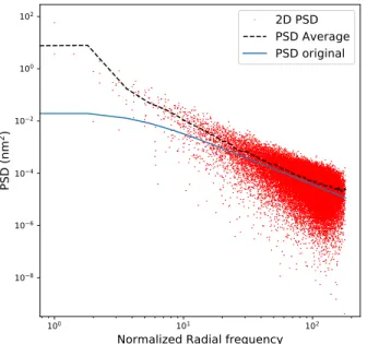
In order to test the validity of the generated map, a PSD was calculated from it, since
P SD = 1
AF{hf(x, y)} . (18)
The 2D values of this PSD were converted into polar coordinates, and compared to the original expression from equation (14) in order to verify the reliability of this method. The results are inFigure 8a.
100 101 102
Normalized Radial frequency
10 8 10 6 10 4 10 2 100
PS
D
(nm
2)
2D PSD
PSD Average
PSD original
(a) Here the height map was originated by the PSD method. The radial average of the 2D PSD is very close to the original line from equation (14), except for the lower frequencies. This separation only appears after applying the mask to the height map.
100 101 102
Normalized Radial frequency
10 8 10 6 10 4 10 2 100 102
PS
D
(nm
2)
2D PSD
PSD Average
PSD original
(b) Here the Zernike Polynomials are added to the height map, thus dominating the lower frequencies. The behaviour of the higher frequencies is dominated by the original PSD from equation (14).
Figure 8: Calculated power spectrum densities (PSD) from a computer-generated height map. Only the values within the footprint are calculated. The red points represent the PSD calculated from the 2D height map, and then translated into polar coordinates. The black dashed line represents the radial average of the red points, and the orange line represents the original function from equation (14). In this case σ0 = 15 nm, P = 2 and ρc = 4
cycles per aperture.
The height maps originated from the Zernike polynomials and the PSD function are then scaled such that their RMS inside the footprint is given by the values of equation (13). Then the three maps are summed into the surface’s form error. The incident wavefront will then gain a phase given by
∆ϕ = (n(λ)− 1)h(x, y)
λ , (19)
or, in the case of a mirror,
∆ϕ = 2h(x, y)
λ , (20)
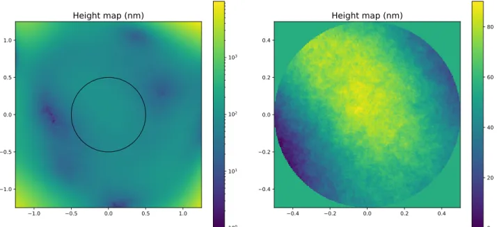
where λ is the wavelength, and n(λ) is the surface material’s refractive index. An example of one of these height maps is inFigure 9.
The reason such a large area is computed (a square of 2.5× 2.5 footprint diameters) is due to the Fourier
propagation. Boundaries too close to the light will cause aberrations due to numerical artefacts, but larger boundaries require either lower resolutions inside the footprint or larger computational resources. Furthermore, some light can hit the surface outside the footprint due to diffraction from the wavefront aberrations, so it would be unrealistic to cut out completely the SFE outside. However, the Zernike polynomials grow very quickly outside the footprint radius and become very dominant. This made some very bright and deformed diffraction patterns appear on the simulations. Therefore we rescaled the radius of the Zernike polynomials to 1.25 (previously it
−1.0 −0.5 0.0 0.5 1.0 −1.0 −0.5 0.0 0.5 1.0
Height map (nm)
100 101 102 103(a) Total height map, including the zones outside the foot-print. The logarithmic scale is necessary in order to visualize effects other than the Zernike polynomials.
−0.4 −0.2 0.0 0.2 0.4 −0.4 −0.2 0.0 0.2 0.4
Height map (nm)
0 20 40 60 80(b) Height map inside the footprint. Low, medium, and high spatial frequencies are clearly noticeable.
Figure 9: Example of a generated height map, with a total RMS on the footprint (inside the circle with diameter 1) of 15 nm.
was 0.5, corresponding to the footprint radius), which was enough to avoid the aberrations.
This representation aims to be as realistic as possible, and, based on the practical experience within the METIS group, this is expected to be an excellent first iteration.9 If in a later phase the manufacturers report
that these specifications can not be realistically mimicked for some of the surfaces, this representation will be adapted, the analysis run again, and the surface quality budgets might need to be revised.
The code behind the generation of the SFE maps was based on the work from Van den Born.11
5. ASSESSING THE IMPACT OF THE TALBOT EFFECT
The Talbot length, given in equation (1), is a function of a spatial frequency and the wavelength. Lower Talbot lengths occur for higher spatial frequencies and are more harmful because amplitude and phase aberrations change quicker. Moreover, since a surface form error has a spectrum of spatial frequencies that extends indeterminately, the lowest Talbot length for a surface approaches 0. However, since the amplitude decreases for higher frequencies, their impact is also lower. We considered that a useful metric for the lowest Talbot length would correspond to the cutoff frequency ρc, so
LlowT = 2 ( 2r0 ρc )2 λmax , (21)
where λmax is the largest wavelength, and r0 is the radius of the surface. However, since all surfaces are
conjugated to the collimated space, r0 is the aperture radius of the system, corresponding to the 19.271 m of the
ELT’s entrance pupil. Incidentally, all surfaces were analysed with the same cutoff frequency, and so all Talbot lengths are the same (around 1.43× 10⁷m for a wavelength of 13 µm). Nevertheless, the most important metric
to evaluate the impact of the Talbot effect is not the Talbot length, but the Talbot number
NT=
z LT
an adimensional number representing the ratio between the propagating distance z and the Talbot length. Using the distances to the pupil (z = d) to calculate the Talbot number, we concluded, before propagation, that the most critical surfaces of the CFO were KM3 (NT = −0.160), the last mirror of the derotator, and FM2
(NT= 0.242), the folding mirror right after it. For the LMS, at λ = 5.2658 µm, the most critical surfaces were
the LMS pick-off (NT=−5.17), and the LMS CM1 (NT=−0.131). As for the IMG, there weren’t any surfaces
that presented especially high Talbot numbers. Incidentally, the surfaces with the highest Talbot number are also the surfaces closest to a focal plane, and so their conjugate is far away from the pupil.
6. RESULTS AND DISCUSSION OF THE PROPAGATION ANALYSIS
Table 2shows the Talbot numbers calculated for the surfaces of the CFO, and up to the first pupil planes of the IMG and the LMS LM and N modes. It is important to notice that this is simply a metric based on the cut off frequency. There is a spectrum of Talbot numbers with prevalence on the lower spatial frequencies (lower Talbot numbers). These results were obtained by using the method ofsection 2.1for 100 different chief rays and calculating the average distances and their standard deviation.
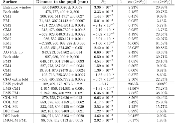
Table 2: Distances to the pupil for the conjugated of the METIS optical surfaces. CMs are curved mirrors, FMs are folding mirrors, KMs are the mirrors of the derotator, COL are the imager colimator mirrors, and DIC are the imager Dichroics. The surfaces of the CFO, the LMS, the common IMG (common path – LM and N), and the IMG LM are separated by horizontal lines. The uncertainties were calculated from the standard deviation of the distances calculated. The largest wavelength was of 13 µm for the CFO, 5.2658 µm for the LMS, 14 µm for the LMS (N band and common path), and 5.5 µm, for the IMG (LM), which, for a cut-off frequency of 4 per aperture (from equation (21)), give a Talbot length of 14284 km, 35263 km, 13263 km, and 33761 km respectively.
Surface Distance to the pupil (mm) NT 1− | cos(2πNT)| | sin (2πNT)|
Entrance window 480548693.0676± 0.0058 3.36× 10⁻² 2.23% 20.98% Back side 475, 777, 400± 2, 300 3.33× 10⁻² 2.18% 20.78% CM1 206, 706, 511.4717± 0.0027 1.44× 10⁻² 0.41% 9.08% FM1 71, 613, 307.21442± 0.00097 5.01× 10⁻³ 0.05% 3.15% CM2 −131, 220, 594.4841 ± 0.0019 −9.18 × 10⁻³ 0.17% 5.77% CM3 −313, 473, 999.7529 ± 0.0048 −2.19 × 10⁻² 0.95% 13.75% KM1 −659, 828, 640.3412 ± 0.0098 −4.62 × 10⁻² 4.19% 28.64% KM2 −986, 552, 550.121 ± 0.014 −6.91 × 10⁻² 9.28% 42.07% KM3 −2, 289, 960, 982.828 ± 0.036 −1.60 × 10⁻¹ 46.66% 84.58% FM2 3, 456, 851, 374.397± 0.051 2.42× 10⁻¹ 95.03% 99.88% AO Pick up 943, 213, 684.802± 0.014 6.60× 10⁻² 8.49% 40.33% Back side 927, 980, 900± 9, 000 6.50× 10⁻² 8.22% 39.71% FM3 648, 517, 001.3746± 0.0093 4.54× 10⁻² 4.05% 28.16% CM4 227, 273, 387.9811± 0.0034 1.59× 10⁻² 0.50% 9.99% CM5 19, 801, 870.77479± 0.00024 1.39× 10⁻³ 0.00% 0.87% CM6 −195, 713, 725.3532 ± 0.0027 −1.37 × 10⁻² 0.37% 8.60%
CFO extra fold −509, 495, 555.7782 ± 0.0082 −3.57 × 10⁻² 2.50% 22.24%
LMS pickoff 182, 409, 173, 973.3± 2.2 −5.17 2053% 2088% LMS CM1 4, 615, 956, 414.881± 0.064 −1.31 × 10⁻¹ 31.96% 73.28% LMS FM1 2, 242, 186, 450.229± 0.027 6.36× 10⁻² 7.88% 38.90% COL M1 879, 758, 732.626± 0.012 6.63× 10⁻² 8.56% 40.46% COL M2 553, 375, 485.4159± 0.0062 4.17× 10⁻² 3.42% 25.90% COL M3 333, 925, 896.9455± 0.0039 2.52× 10⁻² 1.25% 15.77% DIC front 162, 161, 833.9403± 0.0021 1.22× 10⁻² 0.29% 7.66% DIC back 156, 071, 330.3103± 0.0020 4.62× 10⁻³ 0.042% 2.90% IMG-LM FM1 98, 508, 442.0113± 0.0015 2.92× 10⁻³ 0.017% 1.83% The distance values are extremely high because the system magnification is also very high. We are compressing a beam from an entrance pupil of almost 40 m into optical surfaces with a few centimetres. Even so, the Talbot
numbers are somewhat low, because the Talbot length is very large.
Although most Talbot numbers seem to be low, any conclusions must be taken from the impact on the Amplitude and Phase. Equations (7) and (8) show that for an initial phase aberration, the amplitude is affected with the sine of NT, while the phase is affected with the cosine of NT. In other words, the rate by which the
initial aberration is translated into the amplitude is given by| sin (2πNT)|, while the rate it disappears from the
phase is given by 1− | cos(2πNT)|. These values are also onTable 2, and they show that the amplitude is more
affected than the phase.
In fact, out of the 26 surfaces analysed, only 4 have an impact of less than 5% on the amplitude. From the remaining 22, 15 have an impact higher than 20%. Another two have an impact higher than 10%, and 5 have an impact between 5 and 10%. As for the impact on the phase, these values change considerably with only 9 surfaces having an impact higher than 5%. From these, 5 are below 10%, but the remaining 4 (KM3, FM2, LMS pickoff, and LMS CM1, which were mentioned before) have substantial impacts. However, since only these two surfaces are contributing considerably for the reduction of the phase aberrations, it is not expected that the phase will be considerably affected by the Talbot effect. The same cannot be said about the amplitude, where most of the faces are contributing considerably for the amplitude aberrations.
This metric is based on the values for the cutoff frequency only. The values in Table 2do not reflect the changes in the WFE or the amplitude. What can be concluded, though, is that surfaces with large Talbot num-bers decrease the phase aberrations (while increasing the amplitude ones), and surfaces with low Talbot numnum-bers do not have a considerable impact on the phase aberrations (but have some impact on amplitude aberrations). However, the full simulations will also include the diffraction effects of a circular aperture and obscuration, as well as some pupil masks in the optical path. These affect both the phase and the amplitude of the wavefront.
Because the total effect on the phase and amplitude cannot be easily dismissed, we executed the propagation through the whole system. As the worst contributors, KM3, FM2, LMS Pickoff, and LMS CM1 were set to have slightly better specifications than the remaining surfaces, as seen in Table 3. These values were chosen from experience in previous projects,9 but might be revised after future iterations with the manufacturers.
Table 3: Specifications for the SFE of the optical surfaces of the CFO.
Surface Total RMS Cut off frequency PSD slope Zernike 1 indexes Zernike 2 indexes KM3, FM2, LMS Pickoff, LMS CM1 10 nm 4 cycles per aperture 2 2-20 21-54
All others 15 nm 4 cycles per
aperture 2 2-20 21-54
Figure 10 shows the results of one propagation simulation. The grid size was of 1024× 1024 pixels and the
wavelength of 2.9 µm. As it can be seen, the amplitude shows high and medium frequency aberrations, which are not so prominent on the phase. On the other hand, lower frequency aberrations are not present on the amplitude but are visible on the phase. This is expected, as higher frequencies correspond to higher Talbot numbers.
Figure 11shows the phase after a simulation for the same generated height maps, but without any propagation. In other words, the phases of each surface were simply summed, and there are no diffraction nor Talbot effects. The results are similar to the ones inFigure 10b. The main difference is that when there is no propagation, the higher frequencies are much more prominent since they are not translated to amplitude aberrations by the Talbot effect, and there are also no diffraction effects. The root mean square values of the phases are shown in
Tables 4to6.
Looking closely atFigure 10it’s also possible to see diffraction effects on the borders. However this is more outstanding for higher wavelengths, as seen inFigure 12.
The simulations onFigure 12are performed with the same height maps as before, but propagation is done with a wavelength of 13 µm instead. Diffraction effects become much more pertinent, and they almost overwhelm
(a) Amplitude at pupil after propagation. The integral of the squared amplitude is equal to the total energy.
(b) Phase at pupil after propagation. Units are in radians.
Figure 10: Results of the propagation at the exit pupil of the CFO for a wavelength of λ = 2.9 µm.
Figure 11: Wavefront phase at the exit pupil of the CFO without propagation. The wavelength is λ = 2.9 µm. the amplitude aberrations caused by the Talbot effect. The diffraction effects can be isolated by performing a
(a) Amplitude at pupil after propagation. The integral of the squared amplitude is equal to the total energy.
(b) Phase at pupil after propagation. Units are in radians.
Figure 12: Results of the propagation at the exit pupil of the CFO for a wavelength of λ = 13 µm. propagation simulation with ideal surfaces, i.e. without SFE.
The phase RMS was calculated. The simulation generated 32 different height maps for each surface, with a grid size of 1024× 1024 pixels. The results are inTables 4to 6.
Table 4: Simulation results for the phase up to the LMS entrance pupil. Three cases were considered: 1. full propagation was performed and both phase and amplitude varied; 2. no propagation was performed, the amplitude aberrations were not calculated, and the final phase is the sum of the aberrated phases for each surface; and 3. propagation but with ideal surfaces, i.e. without SFE. The simulation was performed with 32 randomly generated sets of height maps. The values presented, including the impact (this is calculated using (23)), are the average and the uncertainties are the respective errors to the mean.
λ Propagation No propagation Ideal propagation
Impact (%) (µm) RMS (nm) PTV (nm) RMS (nm) PTV (nm) RMS (nm) PTV (nm) 5.187 121.4± 5.8 837± 27 122.8± 6.1 695± 27 30.1 524 4.6± 1.6 5.2243 121.5± 5.8 838± 27 30.3 536 4.6± 1.6 5.2282 121.5± 5.8 838± 27 30.3 536 4.6± 1.6 5.2658 121.5± 5.8 841± 27 30.6 522 4.6± 1.6
Table 5: Simulation results for the phase up to the IMG-N. The conditions and the three cases considered are the same asTable 4.
λ Propagation No propagation Ideal propagation
Impact (%) (µm) RMS (nm) PTV (nm) RMS (nm) PTV (nm) RMS (nm) PTV (nm) 7.5 129.3± 4.7 1118± 23 121.9± 5.1 703± 18 46.7 680 1.59± 0.37 10 136.7± 4.4 1254± 23 64.6 837 1.73± 0.56 14 152.4± 4.0 1463± 22 93.5 1072 2.01± 0.92
It’s interesting to notice that RMS2
no propagation+ RMS2ideal≈ RMS2propagation, which seems to indicate that
Table 6: Simulation results for the phase up to the IMG-LM. The conditions and the three cases considered are the same asTable 4.
λ Propagation No propagation Ideal propagation
Impact (%) (µm) RMS (nm) PTV (nm) RMS (nm) PTV (nm) RMS (nm) PTV (nm) 2.9 120.5± 5.6 1088± 88 121.1± 5.6 711± 25 13.5 320 1.41± 0.20 4.0 121.4± 5.5 929± 26 21.5 445 1.62± 0.25 5.0 122.8± 5.4 989± 26 28.7 515 1.79± 0.31 5.5 123.7± 5.4 1010± 26 32.3 520 1.87± 0.35
these two sides can be calculated and compared to the case without a propagation. This serves as a metric to evaluate the impact of the Talbot effect on the phase. This metric should thus be given by
Impactphase= 1− √ RM S2 propagation− RMSideal2 RM Sno propagation . (23)
As expected, the impact shown inTables 4to 6seems to be increasing with the wavelength λ, although the uncertainty is still too large to allow any strong conclusions. Still, according to what the average RMS values seemed to indicate, the impact of the Talbot effect is meagre, under 2% for the IMG, and 5% for the LMS (whose surfaces contain the highest Talbot numbers in METIS, as shown inTable 2). The presented values are calculated using equation (23) for each of the 32 sets of height maps, and not by using the averages of the RMS presented inTables 4to6. However, this is simply a metric that pretends to separate the effects of the diffraction from the propagation phase, and might not be accurate. Furthermore, due to the numerical limitations of the method, there is no simple way of knowing what the boundaries of the exit pupil where these values should be calculated are: the amplitude decreases quickly outside the boundaries, but it never reaches 0, and the phase starts changing too quickly, introducing unreal effects on the RMS. The solution found was to cut the pupil as the same size of the smallest amplitude mask, and further undersize it three pixels. This seemed to be a good solution, but it may be cutting a diffraction ripple from the calculations.
The impact on the amplitude, since the no propagation mode does not return any values or aberrations for the amplitude, needs to be considered differently. Since there are no aberrations for the no propagation mode, the amplitude should present a uniform distribution across the aperture of the pupil S, with an average value for the amplitude A. The amplitude units are defined such that the integral of ∫A2dS = 1. This becomes
∑N
i A
2
i = 1 on a discrete problem, where N is the number of pixels of the aperture, and i the index of such
pixels. When there is no propagation, the amplitude is uniform across the surface, and so N A2 = 1. Since on
these simulations the aperture had N = 755532 pixels, we get that A = 115.0465× 10⁻⁵, as shown in Tables 7
to9. Since there is not an initial amplitude aberration, this value will be used as a reference, and the impact of the Talbot effect is given by
Impactamplitude=
RM Spropagation
1.150465× 10⁻³. (24)
Table 7: Simulation results for the amplitude up to the LMS entrance pupil. Three cases were considered: 1. full propagation was performed and both phase and amplitude varied; 2. no propagation was performed, there are no amplitude aberrations; and 3. propagation but with ideal surfaces, i.e. without SFE. The simulation was performed with 32 randomly generated height maps for each surface. The values presented are the average and the uncertainties are the respective standard deviations.
λ Propagation No prop. Ideal propagation
Impact (%) (µm) RMS (×10−5) PTV (×10−5) (×10−5) RMS (×10−5) PTV (×10−5) 5.187 15.2918± 0.0042 139.50± 0.45 115.0465 15.36 145.5 1.256± 0.041 5.2243 15.2877± 0.0041 139.42± 0.44 15.36 145.5 1.309± 0.038 5.2282 15.2873± 0.0041 139.43± 0.44 15.36 145.5 1.314± 0.037 5.2658 15.2840± 0.0040 139.32± 0.43 15.37 145.2 1.357± 0.035
Table 8: Simulation results for the amplitude up to the IMG-N. Three cases were considered: 1. full propagation was performed and both phase and amplitude varied; 2. no propagation was performed, there are no amplitude aberrations; and 3. propagation but with ideal surfaces, i.e. without SFE. The simulation was performed with 32 randomly generated height maps for each surface. The values presented are the average and the uncertainties are the respective standard deviations.
λ Propagation No prop. Ideal propagation
Impact (%) (µm) RMS (×10−5) PTV (×10−5) (×10−5) RMS (×10−5) PTV (×10−5) 7.5 15.4867± 0.0021 145.31± 0.20 115.0465 15.42 143.0 1.203± 0.020 10 15.5164± 0.0022 142.51± 0.17 15.48 140.7 0.901± 0.028 14 15.5865± 0.0024 139.64± 0.14 15.57 138.4 0.66± 0.042 Table 9: Simulation results for the amplitude up to the IMG-LM. Three cases were considered: 1. full propagation was performed and both phase and amplitude varied; 2. no propagation was performed, there are no amplitude aberrations; and 3. propagation but with ideal surfaces, i.e. without SFE. The simulation was performed with 32 randomly generated height maps for each surface. The values presented are the average and the uncertainties are the respective standard deviations.
λ Propagation No prop. Ideal propagation
Impact (%) (µm) RMS (×10−5) PTV (×10−5) (×10−5) RMS (×10−5) PTV (×10−5) 2.9 15.6764± 0.0045 155.68± 0.24 115.0465 15.25 149.7 3.146± 0.017 4.0 15.5378± 0.0025 152.72± 0.26 15.32 148.5 2.26± 0.013 5.0 15.4958± 0.0021 148.68± 0.23 15.36 145.7 1.803± 0.014 5.5 15.4863± 0.0020 148.01± 0.24 15.37 145.2 1.633± 0.014 We were expecting the impact to increase with the wavelength, as seen with the phase. However, the impact of the Talbot effect for the amplitude is decreasing with the wavelength, except for the LMS (this behaviour of the LMS is still visible for larger ranges of wavelengths). Overall the impact seems to be small, but this metric can’t be directly compared to the one for the phase. An explanation for this decreasing value could be that one of the components of the metric was miscalculated, or simply that the metric is not correct. There doesn’t seem to be any problem with the propagation itself, but it might be possible that some out-of-boundaries Zernike polynomials, or too narrow border values, might affect the diffraction effects on the non-ideal cases, but it is not possible to take further conclusions without more computational expensive and time-consuming simulations.
7. CONCLUSIONS
In this work we performed a Fourier propagation on the optics of METIS. This had the aim of calculating the impact of the Talbot effect on this instrument. We deduced that the surfaces that are closer to the focal planes have more impact than others, so we will have more stringent manufacturing requirements for them. Overall, we were able to conclude that the Talbot effect has a very low impact on the amplitude and phase, of just a few percent. Currently we do not know if this is enough to affect significantly the high contrast image (HCI) modes of METIS, and we are analysing the Talbot simulations presented in this work.
ACKNOWLEDGMENTS
The authors would like to thank all the METIS consortium teams, especially the Optics and CFO teams, for all the fruitful discussions and ideas exchange. The authors would also like to thank Fundação para a Ciências e a Tecnologia for the grant PD/BD/128266/2016 and UID/FIS/00099/2019. Part of this work has also received funding from the European Research Council (ERC) under the European Union’s Horizon 2020 research and innovation programme (grant agreement No 819155).
REFERENCES
[1] Brandl, B. R., Absil, O., Agócs, T., Baccichet, N., Bertram, T., Bettonvil, F., van Boekel, R., Burtscher, L., van Dishoeck, E., Feldt, M., Garcia, P. J. V., Glasse, A., Glauser, A., Güdel, M., Haupt, C., Kenworthy, M. A., Labadie, L., Laun, W., Lesman, D., Pantin, E., Quanz, S. P., Snellen, I., Siebenmorgen, R., and
van Winckel, H., “Status of the mid-IR ELT imager and spectrograph (METIS),” in [Ground-based and
Airborne Instrumentation for Astronomy VII ], Evans, C. J., Simard, L., and Takami, H., eds., 10702, 582
– 596, International Society for Optics and Photonics, SPIE (2018).
[2] Brandl, B., “E-TRE-MET-503-0026: METIS Executive Summary.” METIS deliverable document (Mar 2019).
[3] Talbot, H. and F.R.S., E., “Lxxvi. facts relating to optical science. no. iv,” The London, Edinburgh, and
Dublin Philosophical Magazine and Journal of Science 9(56), 401–407 (1836).
[4] Goodman, J., [Introduction to Fourier Optics ], McGraw-Hill physical and quantum electronics series, W. H. Freeman (2005).
[5] Zhou, P. and Burge, J. H., “Analysis of wavefront propagation using the Talbot effect,” Applied Optics 49, 5351 (Sep 2010).
[6] Krist, J. E., “PROPER: an optical propagation library for IDL,” in [Proc. SPIE ], Society of Photo-Optical
Instrumentation Engineers (SPIE) Conference Series 6675, 66750P (2007).
[7] Lawrence, G. N., “Optical Modeling,” in [Applied Optics and Optical Engineering, Volume XI ], Shannon, R. R. and Wyant, J. C., eds., 11, 125 (Jan. 1992).
[8] Mahajan, V., [Optical Imaging and Aberrations :: Part II : Wave Diffraction Optics ], SPIE Optical Engi-neering Press, Bellingham, Washington, USA, 1st ed. (1998).
[9] Agócs, T., Zuccon, S., Jellema, W., van den Born, J., ter Horst, R., Bizenberger, P., Cardenas Vazquez, M. C., Todd, S., Baccichet, N., and Straubmeier, C., “End to end optical design and wavefront error simu-lation of METIS,” in [Proc. Spie ], Society of Photo-Optical Instrumentation Engineers (SPIE) Conference
Series 10702, 107029O (Jul 2018).
[10] Sidick, E., “Power spectral density specification and analysis of large optical surfaces,” in [Proc. SPIE ],
Society of Photo-Optical Instrumentation Engineers (SPIE) Conference Series 7390, 73900L (2009).
[11] van den Born, J., Quantifying the wavefront error budget of the MICADO ADC using power spectral density