HAL Id: hal-00545567
https://hal.archives-ouvertes.fr/hal-00545567
Preprint submitted on 10 Dec 2010
HAL is a multi-disciplinary open access
archive for the deposit and dissemination of sci-entific research documents, whether they are pub-lished or not. The documents may come from teaching and research institutions in France or abroad, or from public or private research centers.
L’archive ouverte pluridisciplinaire HAL, est destinée au dépôt et à la diffusion de documents scientifiques de niveau recherche, publiés ou non, émanant des établissements d’enseignement et de recherche français ou étrangers, des laboratoires publics ou privés.
What is a Zero-Difficulty Movement? A Scale of
Measurement Issue in Fitts’ Law Research
Yves Guiard, Halla Olafsdottir
To cite this version:
Yves Guiard, Halla Olafsdottir. What is a Zero-Difficulty Movement? A Scale of Measurement Issue in Fitts’ Law Research. 2010. �hal-00545567�
Manuscript under review (December 2010)
What is a Zero-Difficulty Movement?
A Scale of Measurement Issue in Fitts’ Law Research
Yves Guiard
Laboratoire de traitement et de communication de l’information (LTCI) CNRS, Telecom ParisTech, 46, rue Barrault, 75013 Paris, France.
Halla B. Olafsdottir
Laboratoire de traitement et de communication de l’information (LTCI. CNRS, Telecom ParisTech, 46, rue Barrault, 75013 Paris, France.
RUNNING HEAD: MEASURING DIFFICULTY IN FITTS’ LAW
Brief Authors’ Biographies
Yves Guiard is a PhD in experimental psychology with an interest in Fitts’ law and HCI; he is a CNRS directeur de recherche in the Laboratoire de traitement et de communication de
l’information of Telecom ParisTech, Paris, France.
Halla Olafsdottir is a PhD in motor control with an interest in how humans interact with their environment; she is post-doctoral researcher in the Laboratoire de traitement et de
Abstract
Fitts’ law is the well-known empirical relation which states that the time it takes to complete a simple aimed movement varies linearly with movement difficulty, the latter being quantified with an index of difficulty (ID) computed from the ratio of target distance D to target width
W. The paper asks about the level of measurement involved in the two most popular versions
of the ID, the original Fitts ID and the Shannon ID. Analyzing the way these numerical quantities map onto the concrete geometry of a Fitts task, we show that they lack a true physical zero, meaning that their measurement runs on a non-ratio equal-interval scale and that Fitts’ paradigm has been under-constrained so far from the measurement viewpoint.
A simple way to force the independent variable of Fitts' law to run on a ratio scale of measurement is to calculate the ID as a function of relative target tolerance (RTT = W/D), whose zero is physically anchored, rather than relative target distance (RTD = D/W), whose zero is a numerical abstraction. Task difficulty may then be expressed as relative target
intolerance (RTI = 1−W/D), a quantity confined in the 0-1 interval with a physical limit at
100%. Likewise it is advantageous to base the measurement of movement accuracy on relative movement inaccuracy or error (RME = σA/µA), which has a physical zero, rather than
relative movement amplitude (RMA = µA/σA), which does not. Relative movement precision
can then be computed as RMP = 1–σA/µA, a quantity which again varies in the 0-1 interval
with a physical limit at 100%.
We illustrate the practicability of our new measures of task difficulty and movement precision with the data of Fitts’ (1954) classic tapping experiment. The emerging patterns are simple and coherent, and can be modeled with equations whose coefficients are interpretable. We also highlight two implications we think of special relevance to HCI research. One is that, contrary to an old and widely-held belief, the erratic behavior of the y-intercept of Fitts' law reported in the literature should not be a concern because a y-intercept is essentially
uninterpretable in the absence of a physically defined zero on the x axis. The other implication concerns the reciprocal protocol popular in HCI, and which an ISO standard recommends explicitly. Not only is the measurement of movement time and task difficulty less rigorous with the reciprocal than discrete protocol, but a different measure of difficulty is needed.
Keywords
Simple aimed movement, Fitts’ law, task difficulty, movement accuracy, precision, error, scales of measurement, intercept, discrete vs. reciprocal movement.
CONTENTS
Abstract
Keywords
1. WEAKNESS OF THE DIFFICULTY CONCEPT IN FITTS’ LAW RESEARCH 1.1. Fitts’ Task
1.2. The Discrete and the Reciprocal Protocols 1.3. Fitts’ Law
1.4. Multiplicity of Indices of Difficulty
1.5. Terminology: Difficulty vs. Accuracy vs. Inaccuracy 2. THE MEASUREMENT PROBLEM
2.1. Numbers and Physical Quantities 2.2. Levels of Measurement
2.3. What Physical Quantities in the Measurement of Movement Difficulty? 3. PHYSICAL REALITY I: TASK DIFFICULTY AND THE GEOMETRY OF TARGET LAYOUTS
3.1. Back to the Regular Weber Fraction W/D 3.2. Zero Difficulty and Task Reality
3.3. From Tolerance to Intolerance
4. PHYSICAL REALITY II: MOVEMENT PRECISION AND THE STATISTICS OF MOVEMENT ENDPOINTS
4.1. Back to the Regular Weber Fraction σA/µA
4.2. Actual Ranges of Relative Movement Error σA/µA
4.3. Effective Difficulty: A Wobbly Concept
4.4. From Relative Movement Error to Relative Movement Precision
5. HOW PRACTICABLE ARE THE NEW METRICS? AN ILLUSTRATION WITH FITTS’ (1954) TAPPING DATA
5.1. Methods
5.2. Relative Movement Amplitude RMA = µA/σA
5.3. Relative Movement Error RME = σA/µA
5.4. Relative Movement Precision RMP = 1 − σA/µA
5.5. Discussion
6. SOME IMPLICATIONS FOR HCI RESEARCH 6.1. The y-Intercept Debate
6.2. Measuring Difficulty for the Reciprocal Protocol 7. CONCLUDING REMARKS
8. REFERENCES
9. ACKNOWLEDGMENTS
1. WEAKNESS OF THE DIFFICULTY CONCEPT IN FITTS’ LAW RESEARCH 1.1. Fitts’ Task
Fitts (1954), studying simple aimed movement in an experimental tradition that can be traced back to Woodworth (1899), was the first to realize that the difficulty of movement can be quantitatively measured. In his seminal 1954 paper Fitts defined what he called the index of
difficulty (ID) as
ID = log2 (2D/W), (1)
where D and W stand for target distance and target width, respectively. The two relevant lengths D and W being measured on one and the same continuum x, the research problem is inherently one-dimensional. The continuum in question may be the position of a stylus tip or a screen cursor along one spatial dimension, the magnitude of a force applied to a strain gauge, musical pitch (as imagined by Woodworth, 1899), etc.—in fact any continuous variable that can be placed under the voluntary control of a human (Fitts, 1954, Footnote 2 ). The elegance and the generality of Fitts’ simple aimed movement paradigm lay in its extreme simplicity: a person is asked to reach, in a minimum amount of time, a certain target interval xmin ≤ x ≤ xmax
from a certain start position x0.
1.2. The Discrete and the Reciprocal Protocols
To define the two lengths of Equation 1, it is necessary to distinguish the discrete (Fitts & Peterson, 1964) and the reciprocal protocols (Fitts, 1954), represented in the upper and lower parts of Figure 1. x0 x D W x W xmin xmax W D xmin xmax xmax xmin
Figure 1. The two simple measures that define a simple aimed-movement (or Fitts) task, using the discrete (above) vs. the reciprocal protocol (below). In the latter case the direction of the x axis alternates
The reciprocal protocol, which requires participants to concatenate movements in alternate directions, is obviously convenient to experimenters, who can collect fairly large samples of movement time measures in relatively short sessions. However, this protocol has weaknesses from the measurement point of view. One, which Fitts himself pointed to on second thought (Fitts and Peterson, 1964), is that the meaning of the dependent variable is somewhat equivocal, movement time reflecting the duration of three more or less parallel processes: evaluation of the start point error inherited from the preceding movement, execution of the current movement, and planning of the next movement. But the reciprocal protocol also raises a concern about the validity of the measure involved in the independent variable. The spread of movement endpoints that W is supposed to control reflects the confounded variability of the location of both start points and endpoints. This is why in the rest of this paper we reason by default on the discrete, rather than reciprocal protocol.
1.3. Fitts’ Law
Fitts’ (1954) realization that task difficulty can be measured was a crucial step in the history of the topic as it allowed the discovery of the empirical regularity known today as Fitts’ law. Namely, the mean duration of movement (µT) is linearly dependent on the ID. Using Fitts’
own index (Equation 1), Fitts’ law reads
µT = a * log2 (2D/W) + b (2)
where a and b are empirically adjustable coefficients (a>0).
Equation 2 differs in two respects from the conventional notation of Fitts' version of Fitts’ law, which is MT = a*log2(2A/W)+b. First, rather than MT, we write µT to make it
explicit that the dependent variable of Fitts’ law is mean movement time, the mean of a random variable. Second, we express the ratio as D/W rather than A/W for the sake of
consistency. The traditional notation A/W mixes up the mean of a random variable A (which, in Fitts’ law studies, denotes mean amplitude µA) and a systematic experimenter-controlled
variable W. Thus Equation 2 phrases Fitts’ law as the dependency of µT upon two systematic
variables that characterize the task, D and W. An equally consistent alternative it to write the
ID of Equation 2 in terms of µA and σA, the mean and standard deviation of movement
amplitude. Equation 2 then will read µT = a * log2 (µA/σA) + b. To do so is to phrase Fitts’ law
1.4. Multiplicity of Indices of Difficulty
Fitts' law being one of the few quantitative laws of psychology (Kelso, 1992), it comes as no surprise that sustained efforts have been made over the past half-century to adjust the
formulation of the ID so as to improve the accuracy and the robustness of the law. In their widely cited review of the literature Plamondon and Alimi (1997) were able to list over a dozen respectable variants of Fitts’ law equation. For the present purposes we need not be concerned with the mathematical details that distinguish the formulas from one another. Rather, we will retain the basic equivalence class. To our knowledge all variants of Fitts' law assume that the critical quantity from which µT can be predicted is the quotient of the division
of D by W, that is,
µT = f(D/W), (3)
where f denotes a simple monotonically increasing function, linear, logarithmic or power. Two particular instantiations of Equation 3 deserve special attention, being far more popular than all others in Fitts' law research. One is Fitts’ original Equation 2, the other is the so-called Shannon version of Fitts' law:
µT = a * log2(D/W +1) + b. (4)
Equation 2 is the version of Fitts' law that basic-research psychologists have been using by default almost uninterruptedly since Fitts (1954).1 Equation 4, known as the Shannon version of the ID because MacKenzie (1989, 1992) derived it from Shannon’s (1948) Theorem 17, is that which has been popular for two decades in the human-computer interaction community (Guiard & Beaudouin-Lafon, 2004; Soukoreff & MacKenzie, 2004).
Needless to say, data modeling by means of curve fitting is just one aspect of Fitts' law research. The various model equations that have been put forth in the literature correspond to different substantive theories aimed at explaining the law. However, our angle of attack in the present paper being essentially methodological, in the following analysis we will not depart from a theory-agnostic stance.
1
In Fitts’ (1954) view, the ID measured the amount of information conveyed by the movement, hence his recourse to the binary digit unit. After the huge impact of Shannon’s (1948) communication theory, a major pendulum effect took place in the nineteen sixties, affecting psychology no less than other disciplines (Luce, 2003). Fitts' law students, and Fitts was no exception (Fitts & Peterson, 1964), dropped the bit unit as well as the information theoretic explanation of Fitts' law. However, most psychologists have continued up to present to resort to Fitts’ (1954) initial formula, regardless of the fact that the explanation of Fitts' law that is most widely accepted in psychology, the stochastic optimized sub-movement theory of Meyer, Smith, Kornblum, Abrams, and Wright (1988), predicts a power law equation.
1.5. Terminology: Difficulty vs. Accuracy vs. Inaccuracy
It is generally agreed among Fitts' law students that the law expresses a speed-accuracy tradeoff.2 Such an expression, however, is rather informal (Guiard, 2007). In Equations 2-4 the dependent measure of Fitts' law is certainly not the speed of aimed movements, but rather their duration. Likewise, although the fractional expression D/W which appears on the right-hand side of the equations has obviously something to do with movement accuracy, one does not face an obvious measure of accuracy—like, say, the coefficient of variation of
metrologists, or the probabilities of a hit and a false positive in signal detection theory (Green & Swets, 1966). It seems fair to recognize that the division of D by W yields not a measure of difficulty, but rather a certain measure of relative distance.
Note that the term “difficulty”, introduced more or less incidentally by Fitts (1954), is rather casual too. Strictly speaking, Fitts (1954) showed that µT varies linearly with the
amount of information conveyed by the movement, that amount being measured as the logarithm of the inverse of the probability of the target being hit by chance. Fitts thought that the probability in question is given by W/2D, and so he ended up with the formula ID (bits) = −log2(W/2D), which may be simplified into the formula of Equation 1. Although the way Fitts
(1954) measured information in the context of the aimed-movement paradigm has attracted criticism (e.g., MacKenzie, 1989, 1992), he must be credited for the use of a principled and explicit definition of movement difficulty, squarely equated with information. Apart from the Shannon ID of MacKenzie (1989, 1992), which also equates difficulty with information, it is not clear in what sense the various ID formulas based on the ratio D/W that have been
proposed to improve Fitts’ ID (See Plamondon & Alimi, 1997) measure the difficulty or the accuracy of aimed movements. For example Meyer et al. (1988), who viewed Fitts' law as a speed-accuracy tradeoff, assumed implicitly that accuracy is captured in the right-hand side of their equation µT = a*(D/W)1/2 +b, but they offered no explanation.
Below we will be careful about terminology, sticking to some distinctions that have been often ignored in the literature. One is the distinction between task difficulty, defined geometrically, and movement accuracy, defined statistically, two variables whose level of correlation is too imperfect to justify their confounding. The former refers to the target arrangement, the latter to the relative spread of endpoints in a sample of movements. But we
2 In MacKenzie’s fairly extensive Bibliography of Fitts’ law research, an online Web document that lists 310
references up to June 2002 (http://www.yorku.ca/mack/RN-Fitts_bib.htm, February 9, 2010), one finds 37 paper titles including “speed” and/or “accuracy”, 17 of which include both terms (e.g., Crossman, 1957; Meyer et al., 1988, Plamondon & Alimi, 1997; Welford, Norris, & Shock, 1969).
will see that it is also useful to further distinguish intolerance from tolerance and inaccuracy from accuracy (or, synonymously, imprecision from precision).
2. THE MEASUREMENT PROBLEM 2.1. Numbers and Physical Quantities
Measurement is the process of assigning numerals to objects or events according to certain rules (Stevens, 1946). Typically the process consists of mapping the continuum of real numbers onto physical quantities of the real world. The main focus of this article is the correspondence between the ID of Fitts' law, which is an abstract numerical quantity, and the concrete operational quantity this ID refers to.
2.2. Levels of Measurement
A quick reminder of the four basic levels of measurement and accordingly the four categories of variables that are distinguished3 by S.S. Stevens’ (1946) classic theory of measurement is useful.
(1) The lowest level, designated as nominal (or categorical), corresponds to the mere classification of objects that can be sorted but not ranked. For example, in his 1954 study Fitts used three different tasks; that factor amounted to a nominal variable whose modalities were stylus tapping, disc transfer, and pin transfer.
(2) We then have the ordinal level of measurement (e.g., cool, warm, and hot) where the variable (temperature in this instance) has levels that obey a transitive-asymmetry rule (if warm>cool and hot>warm, then hot>cool), so that there is only one correct order. Notice that up to this level nothing is being said about the spacing of the various modalities or levels of the variable.
(3) The third level of measurement is that using an equal-interval scale. One example is temperature on the C° scale, where the difference between 1° and 2° is the same as between 2° and 3°, 11° and 12°, etc. We do have a metric, but our zero is arbitrary (ice melting for the C° scale).
(4) The highest level of measurement is that involving a ratio scale. That most-severely constrained kind of measurement enjoys all the properties of the first three (i.e., its levels are sorted, ranked, and equally spaced), but in addition it has the special property of a
non-arbitrary zero. The classic example is temperature as measured on the absolute (Kelvin)
3 Applying Stevens’ taxonomy to itself, it is easy to see that scale of measurement is a variable of the ordinal
scale, whose zero corresponds to the disappearance of vibratory motion at the atomic level. More familiar examples are distance, duration, and weight, all of which offer, so to speak, a physical stop at zero.
2.3. What Physical Quantities in the Measurement of Movement Difficulty?
When it comes to the zero of some measure, the concern is not the numerical continuum, which of course has a zero, but rather the objects or events that stand on the real-world side of the mapping, the side we call physical. It is easy to see that the measurement of movement time, the dependent variable of Fitts' law, has a physical zero and runs on a ratio scale. However large the stochastic variability, the duration of an aimed movement cannot be negative. The issue is the measurement of difficulty, the independent variable of Fitts' law, which we will examine below in two steps.
In the first place we will have to consider the target layout that experimenters manipulate, characterized by lengths W and D. At issue is what happens in the concrete geometry of relative tolerance W/D when the Fitts and the Shannon IDs are made to vary up and down. A target layout, however, just specifies what participants are requested to do, and all experienced Fitts' law students know that participants do not always produce the
movements requested of them via the target layout. Especially problematic to experimenters is the fact, first reported by Crossman (1957, cited by Welford, 1968, p. 145), that the spread of movement endpoints tends to be smaller than desired with high relative tolerances, and larger than desired with low relative tolerances. Therefore in a second step we will have to take into account the distributions of movement endpoints characterized by the mean µA and
standard deviation σA of movement amplitude, asking how the coefficient of variation σA/µA
behaves as the IDs are made to vary.
3. PHYSICAL REALITY I: TASK DIFFICULTY AND THE GEOMETRY OF TARGET LAYOUTS
3.1. Back to the Regular, Non-Inverted Weber Fraction W/D
In its default form Fitts' law is the statement of a certain dependency of µT upon the
dimensionless ratio D/W. It is interesting to recall that half a century before Fitts, Woodworth (1899), who failed to discover Fitts' law, did detect the special relevance of that ratio.
However, it was the inverse ratio W/D—the Weber fraction, as he called it—that Woodworth called attention to. Why, in the present paper, we will prefer Woodworth’s notation W/D over
the notation D/W, which has been traditional in the literature since Fitts (1954), requires an explanation.
The distinction between the fractional expression D/W and its inverse W/D may be judged rather idle, mathematically speaking. For example no matter in Equation 2 whether the
ID is noted as log2(2D/W) or −log2(W/2D) as these are just two different writings of the same
thing. Experimental psychologists, however, are not mathematicians. As empirical scientists they need to care about the correspondence between the quantities of their formal models and the physical variables they handle in the laboratory. From a psychological viewpoint there is indeed reason to distinguish D/W vs. W/D: the former amounts to a measure of relative target
distance (i.e., D expressed in units of, or scaled to W), the latter amounts to a measure of
relative target tolerance (i.e., W scaled to D).4
It is important to realize that relative target distance D/W and relative target tolerance
W/D do not have the same metrological status. A target layout in which the tolerance is
positive and the distance zero (i.e., W>0 and D = 0, hence D/W = 0) fails to make any sense in a Fitts' law experiment—in such a case no movement whatsoever can be reasonably requested of a participant. In contrast, the limiting case of an aiming task with a
zero-tolerance target located at some non-zero distance (i.e., W = 0 and D>0, hence W/D = 0) can be investigated in practice5 and makes perfect sense conceptually. This case is no other than that studied by Schmidt, Zelaznik, Hawkins, Frank, and Quinn (1979) with their time-matching paradigm. Thus a physical meaning, zero tolerance, can be attached to the zeroing out of Woodworth’s Weber fraction W/D, but not to the zeroing out of the quantity D/W which stands on the right-hand side of conventional Fitts' law equations.
3.2. Zero Difficulty and Task Reality
In the laboratory the difficulty of a Fitts task can be varied only within certain limits, which are clearly apparent in Figure 2. This figure shows the practicable range of variation of relative tolerance W/D, assuming a certain constant value of D. The lower limit is met on the left-hand side at the point where W = 0, hence relative target tolerance W/D = 0. The upper limit is W/D = 2, where the target begins to incorporate the start point, thus annihilating the
4 A glossary is available in Appendix 1.
5 Of course, the condition W = 0 can be realized only approximately in a laboratory (e.g., with a 1-pixel line on a
very necessity of movement.6 In the middle of the figure is shown the balance point where W
= D, and hence W/D = 1, whose interest will be examined in the next section.
Max Min W/D = 0 Zero relative tolerance W/D = 1 Tolerance equals distance Target center Movement start W/D = 2 Target absorbs start point
Figure 2. How relative target tolerance, shown to increase from left to right for a given value of D, is geometrically bounded, in the case of the discrete protocol (it is important to bear in mind that task difficulty increases in the opposite direction, from right to left). The movement is in the upward direction,
the tolerance interval W being marked with a thickened line.
It is clear from Figure 2 that relative target tolerance in discrete Fitts tasks is confined, for geometrical reasons, in the range 0<W/D<2. It should be realized that outside of that range no numerical values delivered by an ID can have physical relevance, for lack of a feasible movement task. The numerical range of IDs being infinite, this is quite an informative result.
Figure 3 shows the numerical values taken by the Fitts and the Shannon IDs as relative tolerance is made to vary. The first important fact is that neither ID accommodates the case of zero tolerance at the leftmost limit of the figure. The calculation of the IDs resting on relative distance D/W, the inverted Weber fraction traditionally used in Fitts' law research, they both suffer the problem of a division by zero at the limit of a totally intolerant target—yet a very meaningful limit, as already remarked with reference to the Schmidt et al. paradigm.
6
One might possibly object that tasks with W/D≥2 are workable since it is common practice to ask experimental participants to aim to target centers. It is a fact, however, that such a case is never investigated in Fitts' law research, and this is unsurprising. The properties of human movement being what they are, participants presented with a target layout such that W/D≥2 and asked to aim to target center could object quite legitimately that only a small proportion of the tolerance made available to them is exploitable (see Section 4.2).
Target center Movement start Max Min -2 -1 0 1 2 3 4 5 6 0.0 0.5 1.0 1.5 2.0 2.5 3.0 Relative tolerance W/D (-) Fitts ID Shannon ID
Figure 3. How the Fitts and the Shannon IDs map onto the geometry of target tolerance in a discrete task.
Turning to the right-hand side of Figure 3, notice that both IDs continue to run downward beyond W/D = 2, irrespective of the fact that from the moment the target has absorbed the start point there is no room left for a Fitts task, and hence for any task-difficulty considerations. The Shannon ID used in Equation 4 never zeroes out, remaining indefinitely positive. For example its value is still 0.01 for W/D = 100, where the target is a hundred times as large as the distance to cover. This fact raises a concern about the meaning of the
y-intercept of Equation 4. For lack of a true zero on the difficulty axis of a Fitts' law plot, the widely-held belief that the y-intercept of Fitts' law (the coefficient b of Equation 4) must be zero seems ill grounded (more on this in Section 6.1).
The Fitts ID used in Equation 2 zeroes out at exactly W/D = 2, a seemingly sensible place to do so. One might be tempted to conclude that the Fitts ID of Equation 2, unlike the Shannon ID of Equation 4, offers a physically realistic zero, but this is not the case. The theoretical point at which the temperature of a body reaches the absolute zero on the Kelvin scale corresponds to the point where atoms will cease to vibrate, not to the disappearance of these atoms. The problem we have here is that it is not difficulty, a property of the movement task, that cancels out at W/D = 2, but rather the very possibility of the task.
Thus it turns out that the two most popular IDs of the literature both fail to have their numerical zero anchored in the physical world, meaning that they both fail to qualify as ratio-scale measures. In fact, the conclusion may be generalized to other IDs. So long as difficulty is defined as an increasing function of relative target distance D/W, it seems impossible to
figure out, in the face of the basic geometry of a Fitts’ task, what zero difficulty might precisely mean.
The simple fact that, using a conventional ID, it is impossible to define the zero of movement difficulty raises a concern about the metric of the independent variable of Fitts' law. One compelling reason why it would be desirable to have a ratio-scale level of
measurement on both axes of Fitts' law plots is that a more severely constraining metric in the assessment of Fitts' law would mean tougher tests of the mathematical descriptions of the law, making it easier to falsify them empirically and, therefore, to reduce the number of competing models (Popper, 1983; Roberts & Pashler, 2000).
3.3. From Tolerance to Intolerance
If the zero of traditional measures of task difficulty is elusive, one clearly sees what a zero-tolerance target is. Thus, still focusing on the case of the discrete protocol of Figure 2, let us reason, not in terms of task difficulty (a function of D/W, to reiterate, a mathematically transformed measure of relative target distance, not a literal measure of difficulty) but rather in terms of relative target tolerance RTT = W/D. Let us assume that the target is 100% tolerant when W = D,which means assigning a maximum to relative tolerance, which now ranges from 0 (a true physical stop) to 1 or 100%.7 An interesting next step to obtain a potentially valid measure of task difficulty is to translate relative target tolerance W/D into relative target
intolerance RTI = 1−W/D, along the lines suggested in a different scientific context by Meehl
(1997).8 Without having had to sacrifice the convenient 0-100% range of variation, we now face an operationally clear definition of task difficulty.
That relative target intolerance zeroes out at W/D = 1 is an assumption, and so the zero of relative target intolerance is arbitrary. However, the upper limit of our new variable, total relative intolerance (1−W/D = 1), does constitute a physical stop: since W/D cannot be less than zero, a task with 1−W/D>1 is impossible.
7 It will become clear in Section 4 that the case W = D constitutes a safe arbitrary 100% of relative tolerance. To
anticipate, we will see that because the coefficient of variation σA/µA cannot approach unity, far from it,
experimenters never attempt to approach such a high level of relative tolerance.
8 Our reasoning in this section capitalizes on an analysis by Meehl (1997) aimed at quantifying the degree of
4. PHYSICAL REALITY II: MOVEMENT PRECISION AND THE STATISTICS OF MOVEMENT ENDPOINTS
Section 3 considered the difficulty-measurement issue from the viewpoint of experimenters who manipulate concrete target arrangements, leading to the conclusion that the range of ID values that have a real-world counterpart is surprisingly limited. Relative target tolerance RTT = W/D has an upper limit at 2 or 200% simply because a target layout in which the start point is included in the tolerance interval does not make sense in the laboratory. However, as will become apparent shortly, only a small part of the range of task difficulties of Figure 2 can be actually handled by humans.
4.1. Back to the Regular, Non-Inverted Weber Fraction σσσσA/µµµµA
This section is just a replica of section 3.1, which showed that while the quotient of D/W does not have a physically defined zero, the quotient of the inverse fraction W/D has one,
corresponding to the zero-tolerance case investigated by Schmidt et al. (1989). Switching now from the task geometry to the movement statistics, we must recognize likewise that σA/µA, but
not µA/σA, has a physical zero. The limiting case where σA = 0 and µA>0, hence σA/µA = 0,
corresponds quite simply to the physically meaningful, if ideal case of a deterministic variable. In contrast, the limiting case where µA = 0 and σA>0, hence µA/σA = 0, does not
refer to anything real—in general, a non-negative random variable x whose mean µx is zero
cannot have a non-zero standard deviation σx. This observation, in our opinion, is a decisive
argument for focusing on σA/µA rather than its inverse in the context of Fitts' paradigm.
4.2. Actual Ranges of Relative Movement Error σσσσA/µµµµA
The Weber fraction σA/µA, a regular coefficient of variation, characterizes relative movement error. 9 In Fitts' law experiments a constant error rate is usually asked of participants in the hope that σA/µA will vary proportionally to W/D, the latter Weber fraction allowing
experimenters to prescribe various amounts of tolerance for movement endpoint variability. However, the possible range of variation of σA/µA is actually much narrower than the range of
variation of W/D displayed in Figure 2, meaning that the desired proportionality of σA/µA to W/D cannot hold. Having acknowledged that the geometry of the Fitts task makes it
impossible for an experimenter to raise W/D beyond 2, we must now consider the other, yet
9 With the discrete protocol, where the location of the start point, placed under experimenter control, is fixed,
movement amplitude A and endpoint error E = A-D have the same standard deviation. This is not exactly true with the reciprocal protocol.
more stringent constraints that arise from the performance limitations of human participants. These constraints further reduce, to a considerable extent, the range of relative tolerances within which the difficulty measurement issue can be tackled in Fitts’ paradigm.
The first important fact is that error rates almost invariably inflate at the highest levels of difficulty (i.e., in the extreme left-hand side region of Figure 2). When experimenters display relatively intolerant target layouts, the movements they obtain from participants tend to be less accurate than desired. An unequivocal illustration is provided by the error rates recorded by Fitts and Peterson (1964) in their classic experiment on discrete aimed movement (Figure 4). When relative target tolerance was less than about 10%, Fitts and Peterson’s participants dramatically over-exploited the amount of tolerance made available to them.
0
5
10
15
20
0.0
0.1
0.2
0.3
0.4
Relative tolerance W/D (-)
Error
rate
(%)
D = 7.62cm D = 15.24cm D = 30.48cmFigure 4. The error rate data reported by Fitts and Peterson (1964) for their discrete-movement task.
The classic treatment of this problem, data adjustment based on the calculation of effective target width We (Crossman, 1956; Welford, 1968; MacKenzie, 1992), leads to a
more realistic measure of the ID. However, in the final Fitts' law plot the correction will have inevitably induced a leftward shift of data points, with the consequence that the µT measures
desired for the highest levels of the ID will be missing.
No less severe constraints take place on the right-hand side of Figure 2, with easier tasks. A task characterized as very easy by the ID criterion is in fact liable to be hard if not squarely unpleasant to participants because of the high energetic cost of the required
movements. Fitts task instructions, vital to the paradigm, urge participants to move as fast as they can, given the tolerance constraint, in every condition. But when relative tolerance is
raised up and up, at some point the participants will inevitably approach their upper limit of movement speed, hence the failure of relative movement error σA/µA to faithfully reflect the
increase of relative tolerance W/D (Guiard and Ferrand, 1998).
Kerr and Langolf (1977)
0.0 0.2 0.4 0.6 0.8 1.0 1.2 1.4 1.6 1.8 2.0 0.00 0.05 0.10 0.15 0.20 0.25 0.30
Relative target tolerance W/D (-) Average speed µA/µT (m/s) D=20.32cm D=30.48cm D=40.64cm D=50.80cm
Figure 5. Average movement speed µµµµA/µµµµT as a function of relative target tolerance W/D in the discrete-movement data of Kerr and Langolf (1977).
To illustrate this speed saturation effect we may for example take the data of Kerr and Langolf (1977), collected in a discrete aimed-movement task (Figure 5). Each distance condition being considered separately, so that the effects can be attributed exclusively to relative tolerance, we see a strong and consistent concave-down curvature in the dependency of average speed µA/µT upon relative tolerance W/D. Extrapolating to the right, it is not too
risky to conjecture that average movement speed would not have further increased very much had Kerr and Langolf raised relative target tolerance beyond 25%.10
Given that speed limitation, it is not surprising that Fitts' law students are generally cautious not to present their participants with too high levels of relative target tolerance. Table 1 shows the minimal and maximal W/D values used in a representative sample of published studies. The median maximum is about 1/3, only one study having taken the risk of
investigating W/D>1/2. The figures reported in the rightmost column of the table express the actually-investigated ranges—i.e., (W/D)max – (W/D)min—as percentages of the geometrically
available range of relative tolerances (which is 2, as shown in Figure 2). Judging by this
10 One cogent reason to indeed expect average speed to level off for higher relative tolerances is that the
energetic cost of movement, which may be estimated as the kinetic energy at peak speed, varies like the square of that speed.
sample of studies, it is hardly 20% of the geometrically practicable range or relative tolerance that is actually used by Fitts' law experimenters.
% utilization of the
min max geometrically available range
Fitts & Peterson (1964) 0.010 0.333 16.1%
Kerr & Langford (1977) 0.013 0.250 11.9%
Jagacinski & Monk (1985) – Joystick 0.040 0.376 16.8%
Jagacinski & Monk (1985) - Helmet 0.053 0.499 22.3%
MacKenzie et al. (1987) 0.011 0.333 16.1%
Andres & Hartung (1989) 0.043 0.500 22.9%
Mohagheghi & Anson (2001) 0.028 1.489 73.0%
median 0.028 0.376 0.168
Table 1
Relative tolerance W/D
Minima and maxima of relative tolerance in a sample of studies of discrete movement
4.3. Effective Difficulty: A Wobbly Concept
The widely accepted adjustment for errors technique, which consists of replacing W with effective width We in Fitts' law equations (Crossman, 1957; Welford, 1968; MacKenzie,
1992), translates nominal, or prescribed difficulty into effective difficulty. To be complete the adjustment needs to be done not just on W but also on D,11 and so, using the conventional notation, the expression one ends up with for the computation of the ID is A/We. The symbol A here referring to the mean of movement amplitude, what we really have here is µA/We. But
notice that this is a somewhat wobbly fractional expression whose denominator We seems to
hesitate between a retrospective characterization of the experimental display (“effective” W)12 and a characterization of the participant’s movements (endpoints spread).
In our opinion it is better tactics to unequivocally distinguish two kinds of physical realities, the operational geometry of the task and the statistics of movement endpoints (which specify what experimenters and what participants really did, respectively) than to try to estimate in retrospect what the former or the latter should have done. There are two equally respectable versions of Fitts' law: one, of special interest to HCI, relates µT (along with error
rate) to the target layout and the other, of special interest to basic inquiries, relates µT (alone)
to the coefficient of variation σA/µA. Since σA is proportional to We, no information loss is
11
This adjustment is moderately important as experimenters usually find µA≅D, with similar error rates for
undershoots and overshoots, suggesting that participants aim at target centers (e.g., Fitts & Peterson, 1964).
12 Conceptually effective width W
e has the form of a retrospective reconstruction. It is the value of W that should
have been used by the experimenter, given an observed (excessive, or insufficient) spread of movement endpoints, to obtain a certain constant error rate, say 4% (MacKenzie, 1992).
entailed by recourse to the consistent expression µA/σA (in fact its inverse σA/µA) in place of
the expression A/We from which it has been a tradition to calculate effective IDs.
4.4. From Relative Movement Error to Relative Movement Precision
We argued in Section 3 that the geometry of Fitts' task is better characterized by W/D than by
D/W as the former, but not the latter, has a physical zero. This led us to consider an alternative
definition of task difficulty, based on relative target intolerance rather than tolerance, that enjoys a physical stop. Turning now to the empirical and statistical sort of physical reality handled by Fitts’ law students, one may follow the same reasoning path.
The quantity σA/µA, just like any coefficient of variation σx/µx computed on any
random variable x, is an expression of relative error, inaccuracy, or imprecision. The specific random variable of interest here is movement amplitude but with the discrete protocol, as already noted, amplitude A and endpoint error E = A−D share the same dispersion (σA = σE).
Since there is virtually no risk that the upper limit σA/µA = 1 be reached in any sample of
movements, we may safely assume that relative error varies in the 0-100% interval. Therefore relative movement error can be converted into what we will call relative movement precision
RMP = 1−σA/µA.Thatmeasure varies in the 0-100% range, just like relative target intolerance RTI = 1−W/D. Like RTI, RMP has an arbitrary zero, but the measure’s upper limit (1−σA/µA =
1) is a physical stop because a coefficient of variation cannot be less than zero.13
5. HOW PRACTICABLE ARE THE NEW METRICS? AN ILLUSTRATION WITH FITTS’ (1954) TAPPING DATA
In this section we use Fitts’ (1954) classic stylus-tapping data as a benchmark for testing the concrete practicability of the new variables whose utility we advocated in the foregoing sections. We introduced four tentative predictors of movement time—namely, relative target tolerance RTT=W/D, relative target intolerance RTI=1–RTT, relative movement error
RME=σA/µA, andrelative movement precision RMP=1–RME (see Appendix 1). Because the
most reliable predictors of movement time are to be found in the actual statistics of the movement, rather than in the mere specification of target distance and tolerance (the
13
One practical reason why we prefer the term precision over the term accuracy, which we hold as a strict synonym, is that the latter has the same initial as amplitude. Reserving the notation A for amplitude, one may then write for example that relative movement precision RMP = 1-σA/µA is computed from relative movement
known effective-width argument of Crossman, 1956, Welford, 1968, and MacKenzie, 1992), below we will ignore RTT and RTI to focus on RME and RMP.
Our aim being simply to illustrate the concrete practicability of our new metrics, we will continue to deliberately leave aside any substantive theoretical issues.
5.1. Methods
Fitts (1954) ran his famous stylus-tapping experiment twice, on two consecutive days. On Day 1 Fitts’ participants used a light, oz (28gr) stylus, and on Day 2 they used a heavier 1-lb (454gr) stylus. Although the two sets of numerical data, which Fitts tabulated in his Table 1 (p. 264), were virtually identical, it has been a tradition in the psychological literature to focus on the data of the light-stylus experiment, and so that first half of Fitts’ tapping data offers itself as a natural benchmark: below we will exclusively consider the data Fitts obtained on Day 1, with the light stylus.
Fitts reported estimates of mean movement time µT averaged over 16 participants for
each of his 16 factorial combination of D and W but he did not actually record the position of movement endpoints. In his Table 1 he just reported the percentages of target misses (1.2% on average for the light-stylus tapping experiment). To estimate µA and σA, both needed in the
current analysis, we proceeded as follows. We capitalized on Fitts’ report (p. 265) that undershoot and overshoot errors were about equally frequent in the light-stylus experiment and simply assumed that µA=D. To infer endpoint spreads from error rates we used the
technique described by MacKenzie (1991, Section 2.5). For each combination of D and W we computed effective width We (corresponding to a fixed 4% error-rate constraint) under the
hypothesis that the endpoint distribution was Gaussian, and then σA as We/4.133.
Our analyses separate the different levels of scale, characterized by D or µA, in
keeping with the recommendations of Guiard (2009). A Fitts' law experiment involves two independent variables, but these are not the lengths D and W that it has been traditional to cross orthogonally in designs, since Fitts (1954). To obtain mutually independent variables one needs a dimensionless, scale-independent specification of task difficulty (e.g., the
quotient of the Weber fraction W/D) and some dimensional measure of task scale or size (e.g., target distance D).
5.2. Relative Movement Amplitude RMA = µµµµA/σσσσA
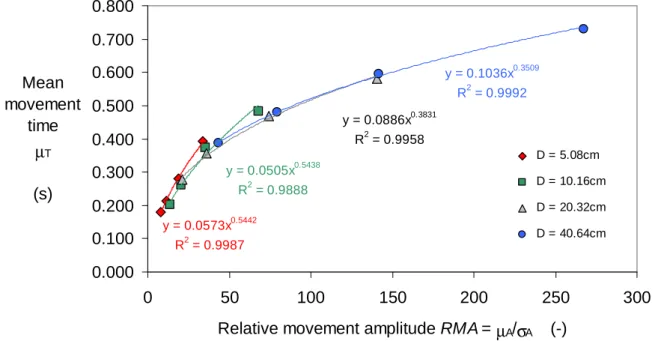
Let us start with the traditional approach. Apart from the fact that we separate the data according to scale level, what is shown in Figure 6 is the basic relation that Fitts' law researchers have traditionally endeavored to understand, that linking µT and RMA. Using
these variables, Fitts’ tapping data is best modeled by a power equation:14
y = 0.0573x0.5442 R2 = 0.9987 y = 0.0505x0.5438 R2 = 0.9888 y = 0.0886x0.3831 R2 = 0.9958 y = 0.1036x0.3509 R2 = 0.9992 0.000 0.100 0.200 0.300 0.400 0.500 0.600 0.700 0.800 0 50 100 150 200 250 300
Relative movement amplitude RMA = µA/σA (-) Mean movement time µT (s) D = 5.08cm D = 10.16cm D = 20.32cm D = 40.64cm
Figure 6. Fitts’ movement-time measures as a function of RMA.
µT = a * (µA/σA) b a>0, b>0 .989<r²<.999. (5)
It follows from Equation 5 that µT=0 for RMA=0. However, if one cares about the mapping of
the equation onto the physical world, this mathematical implication must be judged irrelevant because the zero of RMA, which corresponds to a no-movement condition, fails to qualify as a physical zero (see Section 4.1). Another implication of the equation is that µT=a for RMA=1
(i.e., µA=σA), but this again is of little consequence because 1 is just an arbitrary point along
the continuum of RMA.
5.3. Relative Movement Error RME = σσσσA/µµµµA
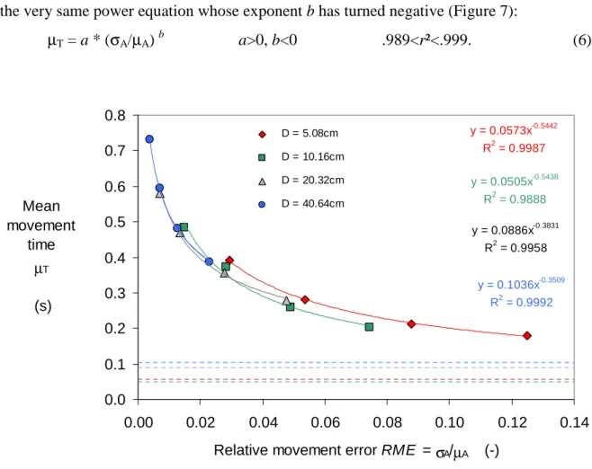
Once the Weber fraction of the x axis has recovered its non-inverted form, becoming a coefficient of variation, Fitts’ tapping data is just as consistent. The best fit is obtained with
14 A logarithmic equation µ
T = a * log (µA/σA) + b, with a>0 and b>0 provides fits that are nearly as good
the very same power equation whose exponent b has turned negative (Figure 7): µT = a * (σA/µA) b a>0, b<0 .989<r²<.999. (6) y = 0.0573x-0.5442 R2 = 0.9987 y = 0.0505x-0.5438 R2 = 0.9888 y = 0.0886x-0.3831 R2 = 0.9958 y = 0.1036x-0.3509 R2 = 0.9992 0.0 0.1 0.2 0.3 0.4 0.5 0.6 0.7 0.8 0.00 0.02 0.04 0.06 0.08 0.10 0.12 0.14
Relative movement error RME = σA/µA (-) Mean movement time µT (s) D = 5.08cm D = 10.16cm D = 20.32cm D = 40.64cm
Figure 7. Fitts’ movement-time measures as a function of RME.
Even though the mathematical model is the same, the metric on the x axis has improved. Now our x variable varies in the 0-1 range, with a zero that corresponds to a true physical stop (σA=0 with µA>0) and with an upper limit that constitutes a physically meaningful, if arbitrary
maximum (RME=1 at σA=µA).
According to Equation 6 µT is undefined for RME=0, due to a division by zero. Notice,
however, that for RME=1 we have µT =a, and this is indeed a physically interpretable result:
the scaling coefficient a of Equation 6 provides an estimate (represented for each movement-scale condition as a dashed line) of the asymptotic minimum of µT that Fitts’ participants
would have been capable of, had they tried to minimize their movement time while totally ignoring the precision constraint (by Equation 6 if RME=1 then µT=a). Given the true zeros
available on both axes, a non-positive value for coefficient a would be hard to tolerate. As a matter of fact, in Fitts’ data the four estimates of coefficient a range quite plausibly in the 50-100ms interval.
5.4. Relative Movement Precision RMP = 1 − σσσσA/µµµµA
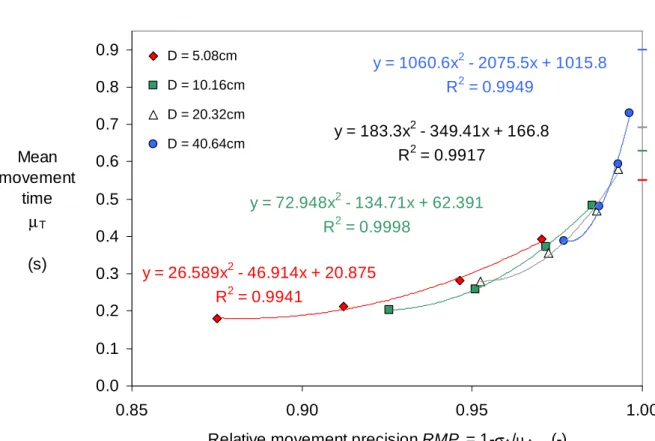
After the complementation to 1 that transforms RME into RMP, Fitts’ data is very accurately modeled by a second-degree polynomial (Figure 8):
µT = a*RMP2 + b*RMP + c .992<r²>.9998 (7)
with a>0, b<0, c>0, and a+b+c>0.
y = 26.589x2 - 46.914x + 20.875 R2 = 0.9941 y = 72.948x2 - 134.71x + 62.391 R2 = 0.9998 y = 183.3x2 - 349.41x + 166.8 R2 = 0.9917 y = 1060.6x2 - 2075.5x + 1015.8 R2 = 0.9949 0.0 0.1 0.2 0.3 0.4 0.5 0.6 0.7 0.8 0.9 0.85 0.90 0.95 1.00
Relative movement precision RMP = 1-σA/µA (-) Mean movement time µT (s) D = 5.08cm D = 10.16cm D = 20.32cm D = 40.64cm
Figure 8. Fitts’ movement time measures as a function of RMP.
It is important to notice that in Fitts’ data, no different in this regard from most data of the literature, the actual x measures cluster in the vicinity of the upper limit of RMP, ranging approximately between .9 and .99. Obviously rightward extrapolation over a short extent to estimate µT at RMP=1 is a great deal safer than leftward extrapolation, over 90% or more of
the RMP range, to estimate µT at RMP=0. 15
The computation of the sum of the three coefficients of Equation 7 yields, for each movement scale level, an estimate of the µT required for perfect precision (if RMP=1 then
15 Mathematically, the coefficient c of Equation 7 is an estimate of µ
T at RMP=0. However, given the very large
amount of leftward extrapolation that the exploitation of this implication of the mathematical model demands, there is no reason to worry about the values obtained from Fitts’ data. Falling in the range 20-1000s (see Figure 8), these estimates are seriously implausible.
µT=a+b+c), the amount of rightward extrapolation being quite moderate. Given the
constraining metrics involved in the relationship, with a physical stop at both µT=0 and RMP=1, there is no question that this sum must be positive. The four estimates a+b+c that
obtain from Fitts’ tapping data (represented on the vertical axis of Figure 8, at RMP=1), again take quite plausible values, in the range 550-900ms.
5.5. Discussion
The results of this new visit to Fitts’ (1954) famous tapping data suggest that recourse to RME and RMP, rather than RMA, entails a benefit and, as far as we may judge, no cost.
On the benefit side, it should be emphasized that the µT vs. RME plot of Figure 7 and
the µT vs. RMP plot of Figure 8 deliver two pieces of information about the performance of
Fitts’ participants that nicely complement each other. While the former plot allowed us to estimate in Fitts’ data the floor of
µ
T for 100% imprecise movements, the latter made it possible to estimate, with remarkably little risk, the ceiling ofµ
T for 100% precisemovements. We do not see how these estimates, both of which seem useful, could have been
obtained in an inquiry based on the traditional RMA-based understanding of movement accuracy in Fitts' paradigm.
But we wish to suggest that this benefit is obtained at no cost. The crucial information contained in a traditional Fitts’ law plot, where the relationship is linearized by expressing µT
as a function of the logarithm of the Weber fraction of the task (or the movement), is its slope in s/bit, the inverse of that slope, in bit/s, being interpretable as an estimate of bandwidth, or throughput (Card, English, and Burr, 1978; Zhai, 2004). The point being made is that the possibility to compute that estimate is not lost in the new approach we have outlined. For example, in a log-log plot the exponent b of Equation 6 will become the slope of a line and, provided that RME is rephrased as information,16 that slope will make it possible to estimate a throughput.
In sum, whereas one can interpret the slope but not the y-intercept of the linear equation of traditional Fitts' law formulas (more on this in Section 6.1), it seems that both coefficients of Equation 6 are interpretable. This, we feel, is good news for researchers who want to detect all the structure of their experimental data, whether their purposes be practical (e.g., comparing the target-reaching performances of computer users provided with different
16 Calculating the entropy of a distribution whose mean and standard deviation are known is a standard exercise
interaction devices or techniques) or basic (improving the rigor of the experimental testing of competing theoretical explanations of Fitts' law).
6. SOME IMPLICATIONS FOR HCI RESEARCH
To recapitulate our main findings, the traditional measurement of task difficulty in Fitts' law research lacks a physical zero, meaning that experimentation has been generally under-constrained so far. This observation may perhaps contribute to explain why it has been so hard thus far to empirically falsify the competing mathematical models of Fitts' law. We suggested that this measurement problem can be fixed by recourse to an alternative definition of task difficulty based on RTT and RTI rather than RTD. The measurement of movement accuracy has also traditionally suffered from the lack of a true zero. We introduced an
alternative definition of accuracy or precision, based on RME and RMP rather than RMA, that appears to fix the problem. We finally showed that using the new measures we propose, consistent and informative patterns are found in Fitts’ well-known tapping data. Below we discuss two specific implications of the foregoing that seem of special relevance to HCI research.
6.1. The y-Intercept Debate
A Fitts' law equation like Equations 2 and 4 includes two empirically determined coefficients. While the slope a quantifies the magnitude of the ID effect on µT over the examined range of IDs, the y-intercept b is supposed to indicate the value of movement time at the point where
difficulty is zero. An ISO9241-9 standard has been published, which specifies “Ergonomic requirements for office work with visual display terminals, Part 9: Requirements for non-keyboard input devices” (ISO, 2000). Soukoreff and MacKenzie (2004), advocating this standard to serve as a methodological guideline for Fitts’ law experimentation in HCI and other applied domains, insisted that even though Fitts' law y-intercept is unlikely to be exactly zero, probably it should not exceed −200 ms (p. 758).
Intuition indeed suggests that this intercept should invariably remain close to zero, but things are not this simple.
Since Fitts’ (1954) seminal paper the appearance of non-zero y-intercepts has never ceased to be a controversial topic in Fitts’ law experimentation. To explain substantial positive intercepts, researchers have for example pointed to the time it takes to tap in place (Zhai, Sue, & Accot, 2002) or to press a mouse button (MacKenzie, 1992), dwell time (Fitts & Radford, 1966), unavoidable delay in the psychomotor system (Fitts & Radford, 1966),
uncontrollable muscle activity in the beginning or end of a movement (MacKenzie, 1992), reaction time (Fitts & Peterson, 1964), modeling errors such as failure to use the Shannon formulation of the ID or recourse to a nominal, rather than effective, measure of W
(MacKenzie, 1989, 1992; Welford, 1960, 1968), random variations in subject performance, or unidentified methodological flaws (Soukoreff & MacKenzie, 2004).
Obviously the case is worst when researchers obtain a substantially negative y-intercept, since a time measure like µT cannot conceivably be less than zero, but that has
happened countless times in the literature (e.g., Epps, 1986; Fitts and Peterson, 1964; Guiard, 1997; Kantowitz & Elvers, 1988; Lazzari, Mottet, & Vercher, 2009, to cite just a few
instances).
It seems that to date no theory has adequatelyexplained why the y-intercept of Fitts' law behaves in fact so erratically and specified how one should handle values that consistently differ from zero, as can be ascertained with appropriate inferential statistical tests (e.g., Sen & Srivastava, 1990). Prior to tackling the issue, we must recall how y-intercepts are calculated from data sets.
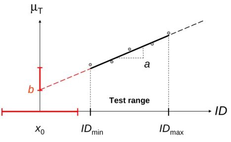
b
µ
TID
ID
minID
maxa
Test rangex
0Figure 9. Distinguishing the line segment fitted over a finite range of IDs to some Fitts' law data vs. the line of infinite length specified by the line’s equation. The data points are arbitrary, and so are the lengths
of the two error bars. Uncertainty about the location of the intercept reflects both the fact that curve linearity is not warranted in the interval of downward extrapolation (vertical uncertainty) and the
metrological irresolution about the location of the zero-difficulty point (horizontal uncertainty).
A Fitts' law equation is a numerical object that experimenters fit to their data by means of linear regression. While the equation specifies a line of infinite length in the graphic plane, a real data set covers a finite interval on the x axis. As experiments never include the case ID = 0, the y-intercept of Fitts' law always relies on downward extrapolation.
Figure 9 helps to understand that the estimation of the b coefficient of Equations 2 and 4 is subject to the combination of two different sources of uncertainty. The intercept being determined by the intersection of the curve with the vertical axis at x = 0, there are two pre-requisites to its estimation: (i) the extrapolation process should not be too adventurous and (ii) one needs to know exactly where the zero of the x variable takes place. Unfortunately, neither pre-requisite is met in the context of Fitts' law.
While any extrapolation from a test range involves a risk (Soukoreff & MacKenzie, 2004), the larger the extent of the extrapolation, the larger the risk. As a matter of fact, it is known that whenever an experiment ventures into low enough ID levels the curve begins to flatten (e.g., Fitts, 1954; MacKenzie, 1992)—not a surprising finding recalling the speed saturation effect of Section 4.2. If one were in a position to take seriously the location of the numerical zero on the horizontal axis, one would have reason to suppose that the b coefficient of Fitts' law tends to under-estimate µT at ID = 0, as suggested by the vertical error bar of
Figure 9. However, one is not in such a position.
In addition to the fact that downward extrapolation from a test range involves an error, we have the serious problem that a Fitts' law plot, as argued in the foregoing, does not offer a physical zero of movement difficulty. From the moment the zero that stands on the ID scale is recognized to be a physically arbitrary point, meaning that the independent variable runs on a
non-ratio equal-interval scale (Stevens, 1946), the numerical value taken by µT at that
particular point must be recognized as arbitrary and uninterpretable. Thus, contrary to an old and widely-held belief, there seems to be no ground for the expectation that, whether Fitts’ law be formulated with the Fitts or the Shannon index, the y-intercept of the law should remain close to zero. As emphasized by Zhai (2004), both coefficients of Fitts' law are indeed needed to summarize a set of data. The coefficient b of Equation 4, which quantifies the level of performance independently of the ID effect, certainly cannot be ignored to characterize a data set, but our analysis reveals that this coefficient, for lack of a true zero of difficulty in Fitts' law, does not satisfy the definition of a y-intercept.
6.2. Measuring Difficulty in the Case of the Reciprocal Protocol
Human-computer interaction, perhaps the field in which the largest amount of Fitts' law research has been taking place in recent past (Guiard & Beaudouin-Lafon, 2004; Soukoreff & MacKenzie, 2004), generally resorts to the reciprocal protocol, which the ISO standard recommends explicitly (ISO, 2000; Soukoreff & MacKenzie, 2004). Thus how the above analysis applies to the reciprocal case seems worth checking.
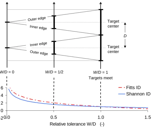
It turns out that the range of ratios of relative tolerance that are geometrically
practicable with the reciprocal protocol is much narrower than with the discrete protocol, as shown in Figure 10. If two targets separated by a constant D are made to expand, they meet each other at the point where W = D hence W/D = 1. At that point the undershoot interval vanishes, leaving no room whatsoever for an aimed-movement task. Thus Figure 10
demonstrates that the range of workable RTT ratios for which the reciprocal version of Fitts’ task can be investigated in actual practice is 0<W/D<1, only one half the range available in the discrete case of Figure 2.
Target center Target center Inner edge Inner edge Outer edge Outer edge D -2 0 2 4 6 0.0 0.5 1.0 1.5 Relative tolerance W/D (-) Fitts ID Shannon ID W/D = 1/2 W/D = 0 W/D = 1 Targets meet
Figure 10. How the Fitts and the Shannon IDs map onto the geometry of target tolerance in a reciprocal task. Compare with Figure 3.
At W/D = 1, the upper limit of RTT for the reciprocal protocol, the Fitts and the Shannon
ID deliver an identical ID = 1, as shown in the lower panel of Figure 10. Since with the
reciprocal protocol it is impossible to raise W/D above 1, it is impossible to reduce the Fitts or the Shannon ID below ID = 1. With the reciprocal protocol neither the Fitts nor the Shannon version of the ID offer a physical zero of movement difficulty. Thus the concern that Figure 2
raised about the meaning of Fitts' law intercept in the discrete case is still more obvious in the reciprocal case.
A quite different, but no less troublesome observation arises from the comparison of Figures 2 and 10. The difficulty level ID = 1, which obtains identically in the case W/D = 1 whether using the Fitts or the Shannon index, corresponds to altogether different task
situations with the discrete vs. the reciprocal protocols. If in the discrete case ID = 1 specifies a rather easy but workable task, in the reciprocal case the same ID = 1 specifies the point at which the two targets meet each other, meaning the technical impossibility of a movement task. This strongly suggests that different measures of task difficulty should be used for the two protocols, an important fact which to our knowledge has been overlooked so far.
A few past studies have sought to compare the performance of discrete vs. reciprocal movements (e.g., Fitts & Peterson, 1964; Guiard, 1997). In retrospect, failure to adapt the calculation of the ID to the markedly different geometries of the discrete and reciprocal tasks casts doubt on their conclusions. More research seems necessary to clarify this point and, more importantly, to elaborate an index of difficulty that will accommodate the different geometries of relative tolerance with the discrete and the reciprocal protocols.
7. CONCLUDING REMARKS
In his seminal Science paper Stevens (1946, p. 679) noted that in psychology, as opposed to physics, “Only occasionally is there concern for the location of a 'true' zero point, because the human attributes measured by psychologists usually exist in a positive degree that is large compared with the range of its variation.” Such is the case obviously with the measurement of task difficulty in Fitts’ law research, as relative target tolerance can only be varied from 1% to 50% or so (Table 1), meaning that relative target intolerance is confined approximately in the 50-99% range.
Stevens (1946, p. 679) continues with the remark that “Intelligence, for example, is usefully assessed on ordinal scales which try to approximate interval scales, and it is not necessary to define what zero intelligence would mean.” In this regard Fitts’ law students seem to be in a better position than students of intelligence. The Woodworth-Fitts paradigm being based on a highly simplified task geometry, it is possible and, we believe, useful to define what zero difficulty and zero precision mean. If, as we have seen, a ‘true’ zero is a prerequisite for y-intercepts to be interpretable, more generally recourse to more constraining metrics of task difficulty and movement accuracy should enhance the quantitative sort of approach that characterizes Fitts’ law research, basic and applied.
8. REFERENCES
Andres, R.O. & Hartung, K.J. (1989). Prediction of head movement time using Fitts’ law.
Human Factors, 31, 703-713.
Card, S.K., English, W.K., and Burr, B.J., (1978). Evaluation of mouse, rate-controlled joystick, step keys and text keys for text Selection on a CRT. Ergonomics, 21, 601 613. Crossman, E.R.F.W. (1956). The measurement of perceptual load. Unpublished Ph.D. thesis,
University of Birmingham, England.
Crossman, E. R. F. W. (1957). The speed and accuracy of hand movements. In E. R. F. W. Crossman & W. D. Seymour (Eds.), The Nature and Acquisition of Industrial Skill, Report to the MRC and DSIR Joint Committee on Individual Efficiency in Industry
[unpublished].
Epps, B.W. (1986). Comparison of six cursor control devices based on Fitts’ law models.
Proceedings of the Human Factors Society 30th Annual Meeting—HFS ‘86. Human
Factors and Ergonomics Society, Santa Monica, CA, pp. 327–331.
Fitts, P.M. (1954). The information capacity of the human motor system in controlling the amplitude of movement. Journal of Experimental Psychology 47, 381-391 (reprinted in
Journal of Experimental Psychology: General, 121, 1992, 262-269).
Fitts, P.M. & Peterson, J.R. (1964). Information capacity of discrete motor responses. Journal
of Experimental Psychology, 67, 103-112.
Fitts, P.M. & Radford, B.K. (1966). Information capacity of discrete motor responses under different cognitive sets. Journal of Experimental Psychology, 71, 475–482.
Green, D.M. & Swets, J.A. (1966). Signal Detection Theory and Psychophysics. Oxford: Oxford University Press.
Guiard, Y. (1997). Fitts’ law in the discrete vs. cyclical paradigm. Human Movement Science,
16, 97-131.
Guiard, Y. (2007). Langage ordinaire et modélisation mathématique: Quelle fonction d’échange dans la loi du mouvement canalisé d’Accot et Zhai? Proc. of the 19th
International Conference of the Association Francophone d’Interaction Homme-Machine.
New York: ACM Press, 11-18.
Guiard, Y. (2009). The problem of consistency in the design of Fitts' law experiments:
Consider either target distance and width or movement form and scale. Proc. of CHI'2009. New York: Sheridan Press, 1908−18.