Synchronverter based HVDC Control in a Multi Machines AC Systems

HAL Id: hal-01421714

https://hal.archives-ouvertes.fr/hal-01421714

Submitted on 22 Dec 2016

HAL is a multi-disciplinary open access archive for the deposit and dissemination of sci-entific research documents, whether they are pub-lished or not. The documents may come from teaching and research institutions in France or abroad, or from public or private research centers.

L’archive ouverte pluridisciplinaire HAL, est destinée au dépôt et à la diffusion de documents scientifiques de niveau recherche, publiés ou non, émanant des établissements d’enseignement et de recherche français ou étrangers, des laboratoires publics ou privés.

Synchronverter based HVDC Control in a Multi

Machines AC Systems

Raouia Aouini, Bogdan Marinescu, Khadija Ben Kilani, Mohamed Elleuch

To cite this version:

Raouia Aouini, Bogdan Marinescu, Khadija Ben Kilani, Mohamed Elleuch. Synchronverter based HVDC Control in a Multi Machines AC Systems. Journal of Electrical Systems, ESR Groups, 2016, pp.515-528. �hal-01421714�

Corresponding author: Aouini Raouia , email: aaouinii@yahoo.com

(1) University of El Manar, L.S.E., LR 11 ES 15, BP 37-1002, Tunis le Belvédère, Tunisie

(2) SATIE-ENS Cachan, 94235 Cachan Cedex, France and IRCCyN-Ecole Centrale Nantes, BP 92101, 44321 Nantes Cedex 3, France (e-mail: bogdan.marinescu@irccyn.ec-nantes.fr) Raouia Aouini1, Bogdan Marinescu2, Khadija Ben Kilani1, Mohamed Elleuch1 Regular paper

Synchronverter based HVDC Control in a Multi Machines AC Systems

The HVDC links are increasingly used not only two distinct power systems but are also embedded into a same meshed AC power system. Thanks to its speed and flexibility, the HVDC technology is able to provide transmission system advantages as transfer capacity enhancement and power flow control. In addition, studies have shown that the way of controlling the HVDC converters impacts the stability of the AC system. This can be particularly exploited to enhance the dynamic power system performances during transients. In this paper, the HVDC emulation by the synchronverter concept is investigated in a realistic power system. A specific tuning method for the parameters of the regulators based on the sensitivity of the poles of the neighbour zone of the HVDC with the respect to the latter parameters is used. As consequence, not only the local performances of the HVDC link, but also overall transient stability of the AC zone in which the HVDC is inserted are improved. Extensive tests are provided using Matlab/Simulink implementation of the IEEE 9 bus/3 machines test system.

Keywords: Synchronverter, Synchronous generator/motor, SHVDC, transient stability, damping oscillatory modes.

1. Introduction

The high voltage direct current (HVDC) link is a mean of transmission of electric power based on high power electronics which offers an opportunity to enhance controllability, stability, and power transfer capability of AC transmission systems [1]. Practical conversion of power between AC and DC became possible with the development of power electronics devices such as thyristors and voltage source converters (VSC). The VSC technology offers even more flexibility, new capabilities for dynamic voltage support, independent controls of active/reactive power and easier integration of wind farms [2].

It was first used in power systems to interconnect asynchronous AC systems as it is the case of the England-France interconnection [3]. Nowadays, HVDC links are increasingly used into a same AC system in order to enhance the grid’s transmission capability and flexibility of the power system. The project Spain-France interconnection [4], which will use the VSC technology scaled up to 2000MW, is such an example. In this context, the HVDC link co-exists with other AC system elements as for instance AC lines and generators.

It was shown that the strategy used to control the HVDC converters can impact the stability of the system in which the link is inserted [5]–[15].

Most control of a VSC-based HVDC system uses a nested-loop d–q vector control approach based on the linear PI technology [15].

Recently in [16], the synchronverter concept has been adapted to the converters of a VSC-HVDC link. The concept of the synchronverter control is to mimic the behavior of a synchronous generator (SG) along with its voltage and frequency regulations [17].

More specifically, the sending-end rectifier emulates a synchronous motor (SM) and the receiving end inverter emulates a synchronous generator (SG). This resulting Synchronverter based HVDC was called SHVDC [16].

In [16], we have taken into account the new context of use of the HVDC during the synthesis of converters controllers. In fact, we have developed an analytic methodology which takes into account, in the tuning stage, the neighbor zone of the HVDC link and the dynamics that most impact transient stability. As a consequence, power system performances were enhanced in addition to local performances. However, the effectiveness of the tuning method of the SHVDC parameters had not been proved in the case of realistic power system.

The present paper shows that the strategy developed in [16] is applicable to a realistic case which is the full model of the IEEE 9 bus system. In the tuning stage, this control technique allows one to take into account dynamic specifications and swing information of the neighbour AC zone in term to better dynamic performances and to improve the transient stability of the neighbor AC zone of the HVDC link; and this fact is proven on a realistic power system.

The rest of the paper is organized as follows: in Section II, the SHVDC structure is recalled. An analytic method to tune the parameters of the controllers of the SHVDC in order to meet the desired performances is given in Section III, while validation tests are presented in Section V.

2. Synchronverter based HVDC

In this Section, the converters of the HVDC line are designed to emulate synchronous machine using the synchronverter concept proposed in [17]. The latter is an inverter of which regulations are chosen such that the resulting closed-loop mimics the behavior of a conventional synchronverter generator (SG) [17]. Therefore, to provide an HVDC structure, another synchronverter working as a synchronous motor (SM) based on the same mathematic derivation is necessary. As a result, the DC power is sent from the SM to the SG.

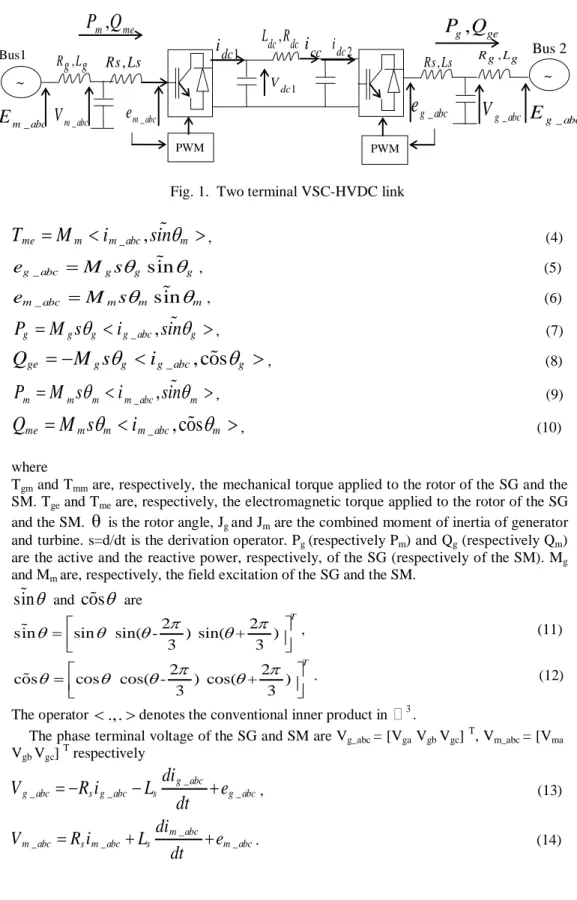
The resulting system in Fig. 1 is called Synchronverter High-Voltage Direct Current (SHVDC). On the figure, we depict:

(i)

the power part of the SG/SM consists of the inverter/rectifier plus LC filter;

(ii) the controls are assured by the electronic part. VSC converter technologies shown in Fig. 2 are used. The overall structure is shown to be equivalent to a SG/SM with capacitor bank connected in parallel with the stator terminal.

As shown in Fig. 2, controllers include the mathematical model of a three-phase round-rotor synchronous machine described by

1 ( ) g gm ge gp g g T T D s J

θ

 = − −

θ

_{, (1)}

1

(

)

m me mm mp m m

T

T

D

J

θ



=

−

−

θ



_{, (2)} _

,

ge g g abc g

T

=

M

<

i

sin



θ

>

, (3)

Fig. 1. Two terminal VSC-HVDC link _

,

me m m abc m

T

=

M

<

i

sin



θ

>

, (4) _

sin

g abc g g g

e

=

M s

θ



θ

, (5) _

sin

m abc m m m

e

=

M s

θ



θ

, (6) _

,

g g g g abc g

P

=

M s

θ

<

i

sin



θ

>

, (7) _

, cos

ge g g g abc g

Q

= −

M s

θ

<

i



θ

>

, (8) _

,

m m m m abc m

P

=

M s

θ

<

i

sin



θ

>

, (9) _

, cos

me m m m abc m

Q

=

M s

θ

<

i



θ

>

, (10) where

Tgm and Tmm are, respectively, the mechanical torque applied to the rotor of the SG and the

SM. Tge and Tme are, respectively, the electromagnetic torque applied to the rotor of the SG

and the SM.

θ

is the rotor angle, Jg and Jm are the combined moment of inertia of generator

and turbine. s=d/dt is the derivation operator. Pg (respectively Pm) and Qg (respectively Qm)

are the active and the reactive power, respectively, of the SG (respectively of the SM). Mg

and Mm are, respectively, the field excitation of the SG and the SM.

sin



θ

and

cos



θ

are

2 2

sin sin sin( - ) sin( + )

3 3 T π π θ _{= } θ θ θ _    , (11) 2 2

cos cos cos( - ) cos( + )

3 3 T π π θ _{= } θ θ θ _    . (12) The operator <.,.>denotes the conventional inner product in

�

3.

The phase terminal voltage of the SG and SM are Vg_abc = [Vga Vgb Vgc] T , Vm_abc = [Vma Vgb Vgc] T respectively _ _ _ _ g abc

g abc s g abc s g abc

di

V

R i

L

e

dt

= −

−

+

, (13) _ _ _ _ m abc

m abc s m abc s m abc

di

V

R i

L

e

dt

=

+

+

. (14) _ m abc

V

, R L_{g g} Bus1 Bus 2 _ m abc

e

_ m abc

E

~

,

m me

P Q

_,

g ge

P Q

PWM PWM 1 dc V 2 dc i 1 dc

i

L R

dc

,

dc _ g abc

e

_ g abc

V

_ g abc

E

cc

i

~ , Rs Ls _{Rs Ls,} Rg,Lg

Fig. 2. Model of the synchronverter: power and electronic parts [17]

The SHVDC given in Fig. 1 is connected to the grid via the impedance (Lg, Rg) such

that _ _ _123

1

(

)

g abc g abc g f

V

i

i

C s

=

−

, (15) _123 _ _

1

(

)

(

)

g g abc g abc g g

i

V

E

R

L s

=

−

+

, (16) _ _123 _ 1 ( ) m abc m m abc f V i i C s = − , (17) _123 _ _ 1 ( ) ( ) m m abc m abc g g i E V R L s = − + , (18) where ig_abc = [iga igb igc] T , ig_abc = [iga igb igc] T

, are respectively the stator phase currents of the SG and the SM, Ls, Rs are, respectively, the inductance and the resistance of the stator

windings and eg_abc = [ega egb egc] T , em_abc = [ema emb emc] T are respectively the back emf of

the SG and the SM.

To mimic the droop of the SG, the following frequency droop control loop is proposed

_

(

)

gm gm ref gp n g

T

=

T

+

D

ω

−

s

θ

, (19)

_

(

)

mm mm ref mp n m

T

=

T

+

D

ω

−

s

θ

. (20)

Tgm_ref is the mechanical torque applied to the rotor of the SG and it is generated by a PI

controller as shown in Fig. 1 to regulate the real power output

P

_g. In the SM case, Tmm_ref is

generated by a DC voltage control for power balance.

_ g ref V ~ _123 g i _ g ref P g M − ge T − n

ω

g θ θ_g 1 J *s g gp

D

(5) (7) (10) Eqn Eqn Eqn 1 k_gs _ gm ref T (22) Eqn 1 s _ e g abc g V (27) Eqn _ g abc

i

_ g abc

e

Bus 2 , s s R L ~

,

g ge

P Q

ge Q − cc i

i

dc2 2 dc V − f

C

_ i g abc g P gq

D

_ g ref Q dc C PWM , g g R L _ V g abc

_ _ _ 1 _ ( i vdc)( ) mm ref p vdc dc ref dc k T k V V s = + − , (21) _ _

(

_

)(

_

)

g g i p gm ref p p g g ref

k

T

k

P

P

s

=

+

−

. (22) The reactive power Qgm (respectively Qmm) is controlled by a voltage droop control loop

using a voltage droop coefficient Dgq (respectively Dmq), in order to regulate the field

excitation Mg (respectively Mm), which is proportional to the voltage generated.

1

(

)

g gm ge g

M

Q

Q

k s

=

−

, (23) g_ref

(

_ ref

)

gm gq g g

Q

=

Q

+

D V

−

V

, (24)

1

(

)

m mm me m

M

Q

Q

k s

−

=

−

, (25) m_ref

(

_

)

mm mq m ref m

Q

=

Q

+

D

V

−

V

, (26) where Vg (respectively Vm), is the output voltage amplitude is computed by

2

3(

)

g ga gb ga gc gb gc

V

V V

V V

V V

=

+

+

, (27)

2

3(

)

m ma mb ma mc mb mc

V

V V

V V

V V

=

+

+

. (28) The circuit equations of the DC line (Fig. 2) are

1 1

1

(

)

dc dc cc dc

V

i

i

C s

=

−

, (29) 2 2

1

(

)

dc cc dc dc

V

i

i

C s

=

−

, (30) 1 2 1 ( ) cc dc dc dc cc dc i V V R i L s = − − . (31) The AC and DC circuits are coupled by the active power relation

1 1 1 dc dc dc

P

=

V i

, (32) 2 2 2 dc dc dc

P

=

V i

, (33) 1 dc m

P

=

P

, (34) 2 dc g

P

=

P

. (35)

Fig. 3. IEEE 9 bus system

3. Control model description

The tuning methodology of the SHVDC parameters developed in [16] is briefly recalled here and enriched such that the local performances are enhanced both for the HVDC as well as for the transient stability of the neighbour AC systems. The resulting control model must preserve the dynamics that most impact the stability of the region neighbouring the HVDC link. For this reason, it was necessary to start from a full model of a sufficient large zone arround the HVDC link. In this study, we considered the realistic of the IEEE 9 bus system.

3.1 Description of the test power system

The IEEE 9 bus system shown in Fig. 3 contains 3 generators, 5 lines, 3 loads and 3 two winding power transformers. The 100 km HVDC cable link has a rated power of 200 MW and a DC voltage rating of ±100 kV [20]. The rating of each generator is 600 MVA and 20 kV. Each of the units is connected through transformers to the 100 kV transmission line. The detailed system data is given in the appendix. The loads L1 , L2 and L3 are modeled as

constant impedances. The simulations tool is in the Matlab/Simulink toolbox.

3.2 Specific framework for the tuning of the SHVDC parameters 3.2.1 HVDC Control Specifications

We first recall the usual full set of control specifications for a VSC-based HVDC. Set-points for the transmitted active power, the reactive power and the voltage at the Set-points of coupling have to be tracked with the following transient performances [15, 18]:

-the response time of the active/reactive power is normally in the range of 50 ms to 150 ms; -the response time for voltage is about 100 ms to 500 ms.

3.2.2 Control objectives

In our previous work [16], we have developed a tuning methodology of the SHVDC parameters which takes directly into account; swing information at the synthesis stage in term of the less damped modes of the neighbor AC zone of the HVDC link. As a consequence, the stability limit in term of the CCT of the neighbor zone was improved in addition to local performances presented above. The local performances are ensured which are tracking of references for active power, reactive power [16]. In this present work, the same tuning method mentioned above is used in the IEEE 9 bus system. More precisely, the synthesis of the SHVDC parameters is done such that the stability performances are ensured for several cases of fault along with the local ones.

� G3 3 4 5 7 8 2 6 100 km 100 km 100 km 1 � G1 � G2 100 km 9 100 km 100 km L1 L2 _L3

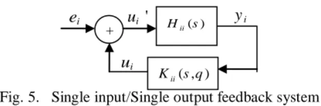
Fig. 4. Feedback system

3.2.3 Control Structure

In order to satisfy these control objectives, the open loop system shown in Fig.3 is put into the feedback system structure presented in Fig.4 where H(s) is the linear approximation of the system in Fig.3.

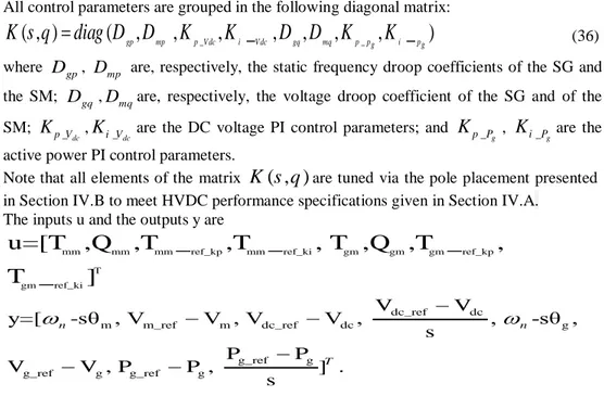
All control parameters are grouped in the following diagonal matrix:

_ _

( , )

(

gp

,

mp

,

p Vdc

,

i

_ ,

Vdc gq

,

mq

,

p p_g

,

i

_ )

p_g

K s q

=

diag D D

K

K

D D K

K

(36) where

D

_gp,

D

_mp are, respectively, the static frequency droop coefficients of the SG and the SM;

D

_gq ,

D

_mqare, respectively, the voltage droop coefficient of the SG and of the SM; _{_} dc p V

K

, _{_} dc i V

K

are the DC voltage PI control parameters; and

K

p P__g ,

K

i P__gare the

active power PI control parameters.

Note that all elements of the matrix

K s q

( , )

are tuned via the pole placement presented in Section IV.B to meet HVDC performance specifications given in Section IV.A.

The inputs u and the outputs y are

mm mm mm ref_kp mm ref_ki gm gm gm ref_kp

T gm ref_ki

u=[T ,Q

,T _

,T _

, T ,Q ,T _

,

T _

]

dc_ref dc m m_ref m dc_ref dc g g_ref g g_ref g g_ref g V V y=[ -sθ , V V , V V , , -sθ , s P P V V , P P , ] . s n n T

ω

− − −

ω

− − −

3.2.4 Regulators parameters and residues

Let

H s

( )

be the transfer matrix of a linear approximation of

∑

and consider each closed-loop of the feedback system in Fig. 5 which corresponds only to input

u

i and

output

y

i.More specifically,

H

ii

( )

s

and

K

ii

( )

s

are the (i,i) transfer functions of H(s), ,

respectively.

Proposition [19]: The sensitivity of a pole

λ

of the closed-loop in Fig. 2 with respect to a parameter

q

of the regulator

K

_ii is

( , ) ii K s q r q λ q

λ

∂ ∂ ₌ ∂ ∂ (37) where

r

_λ is the residue of

H

ii

( )

s

at pole

λ

.

Note that, for our case. (36), ii

( , )

1

s

K

s q

q

_=λ

∂

₌

∂

.

e

_{H s( )}

( , )

K s q

u

u’

y

+

Fig. 5. Single input/Single output feedback system

3.3 Coordinated Tuning of SHVDC Parameters

First, desired locations

λ

_i* can be computed for each pole

λ

_i starting from the control specifications given in Section 3.2.1. The connections between the dynamics of interest and the modes are established based on the participations factors given in Table 1. From the same column of Table 1; several poles have also significant participations to the same dynamic which led us to compute the gains

K

in a coordinated way. More specifically, if

Λ

denotes the set indices j from 1 to 8 for which

H

_jj

( )

s

has

λ

_i as pole, the contribution of each control gain in the shift of the pole is

0 i i ij j j r K

λ

λ

∈Λ = +

∑

, (38) where

λ

_i0 is the initial (open-loop) location of the pole

λ

i and

r

ij is the residue of

( )

jj

H

s

in

λ

_i . Finally, the pole placement is the solution of the following optimization problem 2 * * { , 1...8} arg min j j i i K i K j = =

∑

λ

−

λ

, (39) where

λ

_i is given by (38).

The optimal parameters in the appendix were obtained with (39) solved for the desired locations in Table 1. The specific tuning SHVDC parameters is tested on the IEEE 9 bus/3 machines benchmark [20] shown in Fig. 3.

4. Simulations test

This section deals with performances and robustness of the proposed control. The tuned SHVDC parameters technique presented in the previous Section is tested and compared with the classic vector control. The latter has a cascade structure with a current inner loop more rapid than the outer one. The two controllers are tuned to satisfy the same performance specifications (the usual time setting for HVDC voltage and power control presented in Section 3.2.1). ( ) ii H s ( , ) ii K s q + i e ui' yi i u

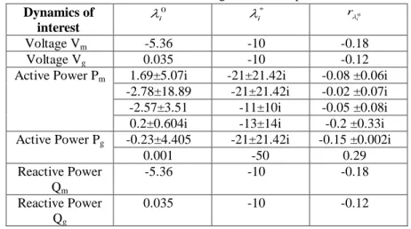
Table 1: Desired modes meeting the HVDC specifications

4.1. Local performances

Table 1 (column 2) presents the desired location of modes

λ

i* for each dynamic of

interest. The optimal parameters K in the appendix was obtained with (39) solved for the desired locations in Table 1. The response of SHVDC for the test power system in Fig. 3 with these tuned parameters is given in Fig. 6 in solid lines in comparison with the ones in dotted lines obtained with a classic vector control. Figs 6.a and 6.b show the responses of active and reactive powers to a +0.1 p.u step in Pg_ref and to a -0.1 p.u step in Qg_ref.. A good

tracking of the active power reference and satisfying control specifications for both responses is observed. It is noted that better dynamic responses are provided with the new coordinated.

4.2. Transient stability

Fig. 7.a, b and c, respectively show the responses of the angular speed of generator G1, G2 and G3, to a three phase short circuit fault of 100 ms duration, occurring near G2. Again better dynamic performances are obtained with the proposed controller: the transient oscillations with the SHVDC control are more damped.

The transient stability is assessed by the Critical Clearing Time (CCT), which is the maximum time duration that a short-circuit may act without losing the system capacity to recover to a steady-state (stable) operation [21].

The obtained CCTs for a three-phase short-circuit occurring near each generator are presented in Table 2 for the classic vector control, and the proposed SHVDC control. We can see that the SHVDC control with tuned parameters improves the transient dynamics of the system and thus augments the transient stability margins of the neighbor network. This is due to the fact that the dynamics of the neighbour zone are taken into account at the synthesis stage via the oscillatory modes in Table 1. The gains of the controllers are computed to damp these modes and thus to diminish the general swing of the zone and not only for the local HVDC dynamics. Dynamics of interest 0 i λ * i λ 0 i r_λ Voltage Vm -5.36 -10 -0.18 Voltage Vg 0.035 -10 -0.12

Active Power Pm 1.69±5.07i -21±21.42i -0.08 ±0.06i

-2.78±18.89 -21±21.42i -0.02 ±0.07i -2.57±3.51 -11±10i -0.05 ±0.08i 0.2±0.604i -13±14i -0.2 ±0.33i Active Power Pg -0.23±4.405 -21±21.42i -0.15 ±0.002i

0.001 -50 0.29 Reactive Power Qm -5.36 -10 -0.18 Reactive Power Qg 0.035 -10 -0.12

(a)

(b)

(c)

Fig.6. Responses of the IEEE 9 bus system (a)Response of Pg to a +0.1 step in Pg_ref (p.u) (a)Response of Qg to a -0.1 step in Qg_ref (p.u) (a)Response of Vg to a +0.1 step in Qg_ref (p.u)

4.8 4.9 5 5.1 5.2 5.3 5.4 0.4 0.45 0.5 0.55 0.6 0.65 time (sec) A c ti v e pow er P g ( p. u)

Classic vector control SHVDC tuned parameters 2.7 2.8 2.9 3 3.1 3.2 3.3 3.4 3.5 3.6 3.7 -0.2 -0.15 -0.1 -0.05 0 0.05 0.1 time (sec) R eac ti v e pow er Q g( p. u)

Classic vector control SHVDC tuned parameters 9.9 10 10.1 10.2 10.3 10.4 10.5 10.6 1.036 1.038 1.04 1.042 1.044 1.046 1.048 1.05 1.052 Voltage Vg [p.u] SHVDC tuned parameters Classic Vector Control

(a)

(b)

(c)

Fig.7. Responses of the angular speed to a 100 ms short circuit near to G2 (a)Angular speed of G2 (p.u)

(b)Angular speed of G1 (p.u) (c)Angular speed of G3 (p.u)

8 9 10 11 12 13 14 15 0.994 0.996 0.998 1 1.002 time (p.u) A ngul ar s peed of G 2 ( p.

u) _{Classic vector control}

SHVDC tuned parameters 6 7 8 9 10 11 12 13 14 15 0.994 0.996 0.998 1 1.002 1.004 time(sec) A ngul ar s peed of G 1( p. u)

Classic vector control SHVDC tuned parameters 8 9 10 11 12 13 14 15 0.992 0.994 0.996 0.998 1 1.002 1.004 time (sec) A ngul ar s peed of G 3 ( p. u)

Classic vector control SHVDC tuned parameters

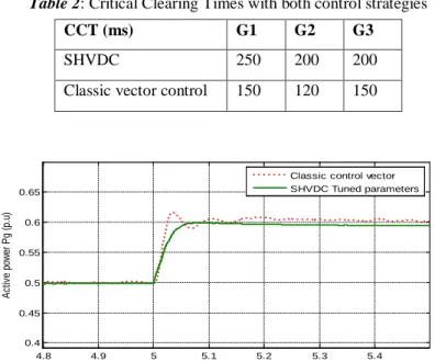
Table 2: Critical Clearing Times with both control strategies

Fig.8. Response of Pg to a +0.1 step in Pg_ref (p.u) with a new operating point

Fig.9. Response of Pg to a -0.5 step in Pg_ref (p.u)

4.3 Robustness against variation of the operating point

As the synthesis of the SHVDC controller is based on the linear approximation as presented in Section III, robustness of performances against the variation of the operating point is required. Therefore, a new load flow setting is considered for the simulations. For example, the active power of load L1 is increased by 50 MW. The gains of the SHVDC controller are not recomputed and are thus the same as in the appendix. Fig. 8 gives the active power response to a +0.1 step in Pg_ref in this case. The latter is comparable with the

one obtained in Fig. 6.a. Indeed, Fig. 9 illustrates the response to a step of -0.5 p.u in Pg_ref

to test the performances of the controller to a sudden change in the direction of the transmitted power. Thus, the dynamic performance is better than the one obtained with the standard controller. These results confirm the good robustness of the performances of the proposed controller against variation of operating conditions.

4.8 4.9 5 5.1 5.2 5.3 5.4 0.4 0.45 0.5 0.55 0.6 0.65 time (sec) A ct iv e pow er P g ( p. u)

Classic control vector SHVDC Tuned parameters 4 4.5 5 5.5 6 6.5 7 -0.8 -0.6 -0.4 -0.2 0 0.2 0.4 0.6 time (s) A c ti v e pow er P g ( p. u)

Classic control vectrol SHVDC tuned parameters

CCT (ms) G1 G2 G3

SHVDC 250 200 200

5. Conclusion

A High Voltage Direct Current HVDC has been emulated using the synchronverter concept. A control strategy of the converters has been proposed based on a specific tuning method which uses, the sensitivity analysis of the system poles with respect to the control parameters. The control strategy has been validated on the realistic IEEE 9 bus benchmark. More specifically, better results than with the standard vector control were obtained for the following points:

- Better dynamic performances (less overshoot and more damping) because this approach allows one to analytically take into account dynamic specifications at the tuning stage. - Better stability margin of the neighbor zone for two reasons. First, swing information is directly taken into account at the synthesis stage in terms of the less damped modes of the neighbor zone and not only for the local HVDC dynamics as it is the case for the standard VSC control.

It is noted that this kind of tuning is surely under optimal in the sense that the constraints to keep the structure of the classical generators and their regulations imposed by the synchronverter principle limits the performances of the .resulting closed-loop.

6. References

[1] Bahrman, M.P.; Johnson, B.K. The ABCs of HVDC transmission technologies, IEEE Power and Energy Magazine, Vol. 5, No. 2, 2007.

[2] Flourentzou, N.; Agelidis, V.G.; Demetriades, G.D. VSC-Based HVDC Power Transmission Systems: An Overview, IEEE Transactions on Power Electronics, Vol. 24, No. 3, 2009.

[3] F. Goodrich and B. Andersen, The 2000 MW HVDC link between England and France. Power Engineering Journal Vol. 1, No. 2, pp 69-74, 1987.

[4] Y. Decoeur, “France-Spain interconnections, first step for smart grids,” Inelfe. Madrid, Spain, Mar. 26th, 2012.

[5] Hauer, J.F.: ‘Robustness issues in stability control of large electric power systems’. Proc. 32nd IEEE Conf. on Decision and Control, 1993, pp. 2329–2334.

[6] Vovos, N.A., Galanos, G.D.: ‘Enhancement of the transient stability of integrated AC/DC systems using active and reactive power modulation’, IEEE Power Eng. Rev.., 1985, 5, (7), pp. 33–34.

[7] Smed, T., Andersson, G.: ‘Utilizing HVDC to damp power oscillations’, IEEE Trans. Power Deliv., 1993, 8, (2), pp. 620–627

[8] Hammad, A.E., Gagnon, J., McCallum, D.: ‘Improving the dynamic performance of a complex AC/DC system by HVDC control modifications’, IEEE Trans. Power Deliv., 1990, 5, (4), pp. 1934–1943

[9] Shun, F.L., Muhamad, R., Srivastava, K., Cole, S., Hertem, D.V., Belmans, R.: ‘Influence of VSC HVDC on transient stability: Case study of the Belgian grid’. Proc. IEEE Power and Energy Society General Meeting, 25–29 July 2010, pp. 1–7

[10] Taylor, C.W., Lefebvre, S.: ‘HVDC controls for system dynamic performance’, IEEE Trans. Power Syst., 1991, 6, (2), pp. 743–752

[11] Latorre, H.F., Ghandhari, M., Söder, L.: ‘Control of a VSC-HVDC operating in parallel with AC transmission lines’. Proc. Transmission and Distribution Conf. and Exposition IEEE, Latin America, 2006, pp. 1–5

[12] Henry, S., Despouys, O., Adapa, R., et al.: ‘Influence of embedded HVDC transmission on system security and AC network performance’. Cigré, 2013

[13] To, K., David, A., Hammad, A.: ‘A robust co-ordinated control scheme for HVDC transmission with parallel AC systems’, IEEE Trans. Power Deliv., 1994, 9, (3), pp. 1710– 1716

[14] Latorre, H., Ghandhari, M.: ‘Improvement of power system stability by using a VSC-HVDC’, Int. J. Electr. Power Energy Syst., 2011, 33, (2), pp. 332–339.

[15] S. Li, T.A. Haskew, and L. Xu, , "Control of HVDC light system using conventional and direct current vector control approaches," IEEE Trans. Power Syst., 2010, 25, (12), pp. 3106–3118.

[16] R. Aouini, B. Marinescu, K. Ben Kilani and M. Elleuch" Synchronverter-based Emulation and Control of HVDC transmission", IEEE Trans. Power Syst, 01/2015. [17] Q.-C. Zhong, and G.Weiss, "Synchronverters: Inverters that mimic synchronous generators," IEEE Trans. Ind. Electron., Apr. 2011, vol. 58, no. 4, pp. 1259–1267.

[18] M-K-S. Sangathan, J- Nehru "Performance of high-voltage direct Current (HVDC) systems with Line-commutated converters", bureau of find Indian standard Manak Bhavan, 9 Bahadur Shah Zafar Marg New Delhi 110002 , April 2013.

[19] G. Rogers, "Power System Oscillations", Kluwer Academic, 2000.

[20] jaikumar Pettikkattil, Simulink Model of IEEE 9 Bus System with load flow, Matlab file ,18 Mar 2014.

[21] P. Kundur, "Power system stability and control", Mc Graw-HillInc, 1994.

7.Appendix

K= [ 55; 46.4; 24.0 ; 28.5 ; 65.64; 58.069; 56.39; 25.11; 37.35].

Parameters of the classic vector control: current loop: kp= 0.6, ki=8, reactive power control: ki=10, active power control: ki=10, DC voltage control: kp=10, ki=10.

Generators: Rated 600 MVA, 20 kV

Xl (p.u): leakage Reactance = 0.18, Xd (p.u.): d-axis synchronous reactance = 1.305, T’d0 (s): d-axis open circuit sub-transient time constant =0.296, T’d0 (s): d-axis open circuit

transient time constant = 1.01 ; Xq (p.u): q-axis synchronous reactance = 0.053, Xq (p.u): q-axis synchronous reactance = 0.474, X’’q (p.u): q-axis sub-transient reactance =0.243, T’’q0 (s): q-axis open circuit sub transient time constant=0.1. M =2H (s): Mechanical starting time = 6.4.

Governor control system : R (%): permanent droop =5, servo-motor: ka = 10/3, ta (s) = 0.07, regulation PID: kp = 1.163, ki= 0.105, kd= 0.

Excitation control system : Amplifier gain: ka = 200, amplifier time constant: Ta (s) = 0.001, damping filter gain kf = 0.001, time constant te (s) = 0.1.

27th AC filter in AC system 1 & 2: reactive power=18 MVAR, tuning frequency=1620 Hz, quality factor=15. 54th AC filter in AC system 1 & 2: reactive power=22 MVAR, tuning frequency=3240 Hz, quality factor=15.

DC system: voltage= ±100 kV, rated DC power=200 MW, Pi line R=0.0139 Ω /km, L=159 µH/km, C=0.331 µF/km, Pi line length= 150 km, switching frequency=1620 Hz, DC capacitor=70 µF, smoothing reactor: R=0.0251Ω , L= 8mH.

Loads: PL1=300 MW, PL2= 300 MW ; PL2= 300 MW

AC transmission lines: Resistance per phase (Ω/km) =0.03, Inductance per phase (mH/km) =0.32, Capacitance per phase (nF/km) =11.5