Mobile Robot Navigation and Obstacles Avoidance based on Planning and Re-Planning Algorithm

HAL Id: hal-01714850

https://hal.archives-ouvertes.fr/hal-01714850

Submitted on 23 Feb 2018

HAL is a multi-disciplinary open access

archive for the deposit and dissemination of

sci-entific research documents, whether they are

pub-lished or not. The documents may come from

teaching and research institutions in France or

abroad, or from public or private research centers.

L’archive ouverte pluridisciplinaire HAL, est

destinée au dépôt et à la diffusion de documents

scientifiques de niveau recherche, publiés ou non,

émanant des établissements d’enseignement et de

recherche français ou étrangers, des laboratoires

publics ou privés.

Mobile Robot Navigation and Obstacles Avoidance

based on Planning and Re-Planning Algorithm

Mehdi Mouad, Lounis Adouane, Djamel Khadraoui, Philippe Martinet

To cite this version:

Mehdi Mouad, Lounis Adouane, Djamel Khadraoui, Philippe Martinet. Mobile Robot Navigation

and Obstacles Avoidance based on Planning and Re-Planning Algorithm. 10th International IFAC

Symposium on Robot Control (SYROCO’12), Sep 2012, Dubrovnik, Croatia. �hal-01714850�

Supported by FNR (Fonds National de la Recherche - Luxembourg) and ANR (Agence Nationale de la Recherche)

Mehdi Mouad§*, Lounis Adouane§, Djamel Khadraoui*, Philippe Martinet§

§ _{Institut Pascal, UBP-UMR CNRS 6602, Clermont-Ferrand, France ;}

E-mail : firstname.lastname@univ-bpclermont.fr

*_{CRP Henri Tudor, 29 avenue John F. Kennedy. L-1855 Luxembourg-Kirchberg ;}

E-mail : firstname.lastname@tudor.lu

Abstract: This paper deals with a multi-mode control architecture for robot navigation and obstacle

avoidance. It presents an adaptive and flexible algorithm of control which guarantees the stability and the smoothness of mobile robot navigation dealing with unexpected events. Moreover, the proposed Planning and Re-Planning (PRP) algorithm combine the two schools of thought, the one based on the path planning to avoid obstacles and reach the target, described as cognitive, and the second using the reactive algorithms. In fact the mix of these two approaches allows us to develop a very reliable algorithm. It provides us a scalable mobile robot navigation and obstacle avoidance, with less processing. It is accomplished by making an initial path planning, then to resolve the problem of unexpected static or dynamic obstacles while tracking the trajectory. A system of hierarchical action selection allows us to switch to a reactive avoidance, then to re-plan a new and safe trajectory to reach the target. A large number of simulations in different environments are performed to show the efficiency of the proposed PRP algorithm.

Keywords: Control Architectures, Obstacles Avoidance, Planning and Re-Planning, Reactive Avoidance.

1. INTRODUCTION

Controlling mobile robots in uncertain environments is of a central importance to many important fields, and calls for many disciplines such as path planning, path tracking and obstacle avoidance.

Navigation in unfamiliar environment needs to give the robot the ability to generate its action plan and to track it. The literature presents different methods of path planning in robotics, like Artificial Potential field method as described in Khatib et al. (1986), Arkin et al. (1989), where robot actions are guided by the sum of attractive and repulsive fields generated respectively by the target and the obstacles. Cell decomposition method cf. Lingelbach et al. (2004 a,b), which consists on decomposing the robots configuration plan on a set of adjacent connected areas from where a graph is generated, the planning consists on exploring this graph and detecting the adjacent areas. Another planning method called Vector field histogram developed by Hafner et al. (2000) and Nehmzow et al. (2000), based on a grid representing the environment each cell contain a value representing the probability of obstacle presence, to plan a path we choose the nearest direction to the target direction which doesn't contain obstacle.

To have an efficient path planning, we need to provide to the robot a precise obstacle map of the environment at the planning moment. Since it is impossible in most of robotic

contexts, it is necessary for the robot to carry a motion planner cf. Belta et al. (2005), Conner et al. (2006). For each environment changing the planner can recalculate a new path; however in certain circumstances this may not be appropriate, because these algorithms generally have a lack of responsiveness. Indeed, the obstacles are often discovered late and plan generation is a time consuming operation. We must therefore stop the robot to start the process of re-planning but this is not a solution in the case of moving obstacles, or when the stop distance is too long.

Control software architectures are usually classified into three main categories as shown in Ridao et al. (2001):

- Reactive vs. Cognitive (deliberative) architectures, many modules connects several inputs sensors/actuators, each module implements a behaviour. These behaviours are called “reactive” because they provide an immediate output of an input value, and cognitive otherwise cf. Brooks et al. (1986), Rosenblatt et al. (1997).

- Hierarchical vs. Non-Hierarchical architectures, the hierarchical architectures are built in several levels, usually three. Decisions are taken in the higher level; the intermediate level is dedicated to control and supervision. The low level deals with all periodical treatment related to the instrumentation, such as actuator control or measuring instrument management (Lumia et al. (1990)).

- Hybrid architectures are a mix of the two previous ones such as Ridao et al. (2001) has described. Usually these are structured in three layers: the deliberative layer, based on planning, the control execution layer and a functional reactive

(1) layer (Schneider et al. (1998)). It's in the same time reactive

with a cognitive level (planning for example).

Several robot control architecture prefer then to base their navigation on a reactive navigation where the control of the actuators is directly coupled with the perception of the environment (Toibero et al. (2007)). This allows the inclusion of very fast dynamic phenomena of the environment as described these works Minguez (2008), Egerstedt et al. (2002), Belta et al. (2005), Conner et al. (2006), Stuart et al. (1996), Lim et al. (2002). These architectures, does not include internal representation of the environment state; make it difficult to plan a sequence of actions to reach a goal. We propose to combine the two approaches according to the context. The architecture is constructed with modular and bottom-up approach as developed by Adouane et al. (2006) and contains a planner with a model of the environment that generates a trajectory, and then when an obstruction is encountered, a reactive avoidance is triggered. Meanwhile the environment map is enriched and a new trajectory is calculated and followed after the obstacle avoidance. This combination allows us to benefit of the advantages of the two approaches to safely generate a new solution to deal with unexpected events.

The proposed Planning and Re-Planning (PRP) algorithm uses in a first time an off-line path planning algorithm based on the principle of artificial potential fields, taking into account the known obstacles in the environment, and the limit cycles based approach for obstacle avoidance algorithm for reactive avoidance of unexpected obstacles cf. Stuart et al. (1996), Khalil et al. (2002). The proposed algorithm provides reliable and continuous robot navigation with less processing. The rest of the paper is organized as follows. Section II gives the specification of the task to achieve. The details of the proposed PRP algorithm are given in section III. In section IV we present in details the transitions criteria and hierarchical action selection of our PRP algorithm, whereas section V describes and analyses the simulation results. We end this paper with conclusion and future works.

2. NAVIGATION IN PRESENCE OF OBSTACLES Navigation is a fundamental problem in mobile robotics. The local navigation problem deals with navigation on the scale of a few meters, where the main problem is obstacle avoidance.

The ultimate goal is the capability of achieving coordinated movements and of carrying out tasks that usually require human assistance. This need for autonomy requires from the robot a certain capacity of being able at any moment to assess both its state and its environment that are usually combined with different other robots states as well as with its mission requirements in order to make coherent control decisions. If we consider navigation aspects, autonomous mobile robots are usually embedded with sensors/actuators according to the mission to be performed. This complexity induces major challenges both at the development of robotics control architecture system but also at the design of navigation software.

Indeed, an autonomous mobile robot has to carry out a set of sensors/actuators dedicated to its own navigation and another sensor set that can change according to the mission to be performed. Therefore the navigation software developed for these vehicles become complex and requires a design methodology.

The unexpected obstacles detection is not addressed in this paper, we use obstacle detection algorithm developed in a previous work cf. Vilca et al. (2012).

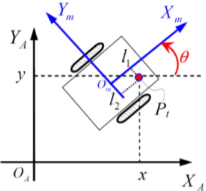
Before describing our PRP algorithm, let’s show the use kinematic robot model (cf. Figure 1):

0 1 . With:

, , : Configuration state of the unicycle at the point “ ” of abscissa and ordinate ( , ) according to the mobile reference frame ( , ! ),

: Linear velocity of the robot at the point “ ”, : Angular velocity of the robot at the point “ ”.

Figure 1. Robot configuration in a Cartesian reference frame. 3. TRANSITIONS AND HIERARCHICAL ACTION

SELECTION

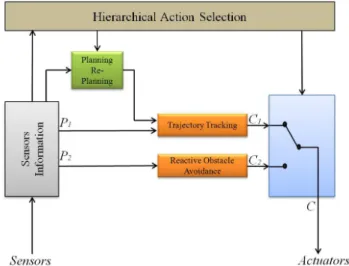
The figure (2) describes the functioning mechanism of our hierarchical action selection, it is organized as follows: • Planning and Re-Planning Module: dedicated to plan a

safe trajectory for the mobile robot, and re-plan on demand.

• Sensors Information data base: in which navigation data is stored.

• Trajectory tracking and Reactive obstacle avoidance: controllers implementing two behaviours respectively, the trajectory tracking and the reactive obstacle avoidance.

• Hierarchical Action selection module: is connected with the sensor information data base in order to assess the robot’s environment data in real time. It has another connection with the planning/re-planning module to

control the re-planning action. Its last connection is with a switch to choose the controller needed and apply its behaviour.

The trajectory tracking controller is the default activated controller. The Hierarchical Action selection module activates the reactive obstacle avoidance controller as soon as it exists at least one obstacle that can obstruct the future robot movement toward the target, and ask for a re-planning of a new trajectory after the robot has avoided the obstacle (value of _" positive as shown in figure 9), then switch to trajectory tracking to track the new trajectory. This allows us to decrease the time to reach the target especially in cluttered environments, and lower the processing volume. Thus, we hierarchically give a priority to each behaviour, and choose to apply a specific one, depending on the situation and its priority.

Figure 2. Control architecture for mobile robot navigation. 4. PLANNING AND RE-PLANNING ALGORITHM The objective of proposed PRP algorithm is to obtain safe, smooth and fast robot navigation in order to be able to navigate through the environment from Point A to point B; the robot should be able to choose an action that maximizes its chances of getting to its goal. Our PRP algorithm relies on three main algorithms that are: off-line path planning, trajectory tracking algorithm and the orbital reactive obstacle avoidance, with determined transitions in a context of hierarchical action selection, it consists of three main stages.

4.1 Off-line path planning

When the navigation goal is specified, we compute a first quick off-line path planning, based on the well-known principle of artificial potential fields. It takes into account the known obstacles in the environment cf. Khatib et al. (1986), to generate an initial trajectory to track. We assume that the robot actions are guided by the sum of attractive field generated by the goal, and the repulsive field generated by each obstacle.

The figure (3) shows an example of path planning with artificial potential fields algorithm.

The attractive force is defined as follow (cf. Figure 4): Uatt(q) = ξ ρgoal(q).

With q the state of the mobile robot, ξ a positive scalar and ρgoal(q) the Euclidian distance: ||q-qgoal||. The function Uatt(q) is positive or null, and reaches its minimum qgoal, where Uatt(qgoal)=0.

The force Fatt is differentiable and: Fatt(q) = -

∇

∇

= - ξ (q-qgoal) / || q-qgoal ||.

Figure 3. Trajectory generation by the artificial potential fields algorithm.

Figure 4. Shape of attractive field. The repulsive force is defined as follow cf. Figure 5): Urep(q) = ½ η ( 1/ρ(q) – 1/ρ0)² if ρ(q) < ρ0.

= 0 if ρ(q) > ρ0.

ρ0 is the distance of influence of the obstacle. The function Urep is positive or null and tends to infinity when approaching the boundary of the obstacle.

Frep(q) = -

∇

= η (1/ρ(q) – 1/ρ0) 1/ρ²(q)

∇

= 0 if ρ(q) > ρ0.

Figure 5. Shape of repulsive field.

Once the initial trajectory is computed, we activate the tracking algorithm to permit to the robot to track its trajectory. If an unexpected obstacle is detected while

(

)

(

)

(

)

(

)

(

)

(

)

(

)

(

)

tracking the trajectory, we send a transition to switch to the reactive avoidance.

4.2 Trajectory tracking

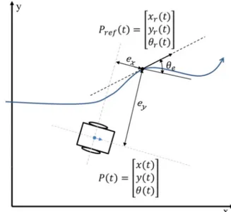
In the used trajectory tracking algorithm we apply command laws described in Maalouf et al. (2006). Knowing that the kinematical model of a differentially wheeled mobile robot in Cartesian coordinates is given by eq. (1) (while using 0), the objective is to track a virtual reference robot which has respectively _$ % & _$ as its linear and angular velocities: ' $$ $ ( )cossin $$ 0 0 0 1/ 0 $ $1.

Then the error variables 2₃, 2₄, and 2₅ that correspond to the instantaneous errors in posture variables are chosen as:

)2234

25

/ 6 ) $$ $

/, with 6 ) cossin cossin 00

0 0 1/.

Equation (12) corresponds to the errors in posture according to local reference frame of the robot (cf. Figure 6). The transformation matrix A converts global coordinates to local coordinates. While using the derivatives of the errors using the constraint _$sin _{$ $}cos _$ and 2_{5 $} , we obtain: '2243 25 ( )01 0 / 7 24 23 18 ) $cos 25 $sin 25 $ /.

From this equation (13), the aim of the control law is to make the errors converge to zero. The used velocity inputs

9% & 9of the control law are (Maalouf et al. (2006) and Kanayama et al. (1990)):

9 $cos 25 :323.

9 $ $:424 :5sin 25.

By substituting ₉ and ₉ in the error of eq. (12) we get:

'2234 25 ( ; < < < = 24 $ $>:424 :5sin 25? :323 23 $ $>:424 :5sin 25? $sin 25 $>:424 :5sin 25? @A A A B .

The proof is based on the choice of Lyapunov function: C >23 24? D1 cos D25EE/:4. Deriving V with respect of time gives us: C :323 GHIJK

L_MH GN O 0.

Given that :₃, :₄, and :₅ are all positive constants, the above inequality would be satisfied and the system with the control law would be stable. The null result corresponds to the equilibrium point where 2₃ 2₄ 2₅ 0.

4.3 Reactive Obstacles Avoidance

The reactive avoidance algorithm is activated when an unexpected obstacle is detected, it’s based on the orbital

Figure 6. Parameters of the error model

obstacle avoidance algorithm and provides a scalable avoidance with several mechanisms to prevent oscillations, local minima and dead end robot situations. The proof of controllers stabilities are given using Laypunov functions cf. Adouane (2009).

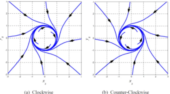
To perform the obstacle avoidance behaviour in our algorithm, the robot needs to fellow accurately limit-cycle vector fields, these vector fields are given by two differential equations:

For the clockwise trajectory motion (cf. Figure 7.a):

I I IDPQ I IE.

I I IDPQ I IE.

For the counter-clockwise trajectory motion (cf. Figure 7.b):

I I IDPQ I IE.

I I IDPQ I IE.

Where (x_S, y_S) corresponds to the position of the robot according to the center of the convergence circle (characterized by R_V radius).

(

)

(

)

(

)

(

)

(

)

(

)

(

)

(

)

Figure 7. Shape possibilities for the used limit-cycles cf. Adouane (2009).

To implement such kind of obstacle avoidance it is important to:

• Detect the obstacle to avoid.

• Give the direction of the avoidance (clockwise or counter-clockwise).

• Define an escape criterion which defines if the obstacle is completely avoided or not yet.

All these different steps must be followed and applied while guaranteeing that: the robot trajectory is safe, smooth and avoids undesirable situations as deadlocks or local minima; and that the stability of the applied control law is guaranteed. The necessary steps to carry out the obstacle avoidance algorithm are given below:

1) Among the set of disturbing obstacles (which can constrain the robot to reach the target), determine the closer to the robot. This specific obstacle has the following features: radius P_"J and ( _WXI , _WXI ) position. 2) After the determination of the closest constrained obstacle, we need to obtain four specific areas (cf. Figure 8) which give the robot behaviour: clockwise or counter-clockwise obstacle avoidance; repulsive or attractive phase. To distinguish between these four areas we need to:

• define a specific reference frame which has the following features (cf. Figure 8):

i. The X_Z axis connects the center of the obstacle (x_[\S],y_[\S]) to the center of the target. This axis is oriented towards the target.

ii. The Y_Z axis is perpendicular to the X_Z axis and it is oriented while following trigonometric convention.

• Apply the reference frame change of the position robot coordinate Dx, yE_{_} (given in absolute reference frame) towards the reference frame linked to the obstacleDx, yE_Z. The transformation is achieved while using the following homogeneous transformation: `34 ab c d d 0 WXI d d 0 WXI 0 0 00 10 01 e `34 ab.

Once all necessary perceptions are obtained, one can apply our obstacle avoidance strategy. To obtain the set-points, it is necessary to obtain the radius “R_V” and the direction “clockwise or counter-clockwise” of the limit-cycle to follow. The position (x_Z, y_Z) gives the configuration Dx, yE of the robot according to obstacle reference frame. The definition of this specific reference frame gives an accurate means to the robot to know what it must to do. In fact, the sign of x_Z gives the kind of behaviour which must be taken by the robot. In repulsive phase, the limit-cycle takes different radii to guarantee the trajectory smoothness. The sign of y_Z gives the right direction to avoid the obstacle. Indeed, if y_Z ≥ 0 then apply clockwise limit-cycle direction else apply counter-clockwise direction. This choice permits to optimize the length of robot trajectory to avoid obstacles. The stability proofs are described in Adouane (2009).

4.4 Re-Planning

While avoiding the obstacle, the sign of robot’s abscissa in the obstacle frame vary, it gives us the switch moment, then we consider that the robot has avoided the obstacle when its abscissa in obstacle frame has a positive value.

Once the robot has accomplished the reactive avoidance, we send a transition to make the Re-Planning from the first positive value of the robot’s abscissa in the obstacle frame; it consists to another call to the planning algorithm which provides a new safe trajectory. After that, we can track our new path to the target (cf. Section 5).

Figure 8. Control architecture for mobile robot navigation. 5. SIMULATION RESULTS

In what follow we present some graphical illustrations describing the simulation results of our proposed Planning and Re-Planning algorithm, showing its reliability and effectiveness. These simulations were implemented in Matlab environment, and by a core 2 duo computer (2.00 GHz, 1.99 GHz, 1.96 GB of RAM).

We first tried to simulate a simple planning and re-planning scenario to compare its results with what we have obtained with our PRP algorithm. The problem we encounter with this test simulation is that we couldn’t have a continuous navigation when detecting an unexpected obstacle. Indeed,

O A

-1

we were forced to stop the robot to get the time to re-plan a new trajectory; because the robot’s stop time was too long (cf. Figure 9).

Figure 9. Illustration of a simple planning and re-planning result.

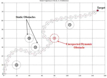
The figure (10) describes an autonomous navigation of the mobile robot. It begins by an off-line path planning followed by a reactive obstacle avoidance as soon as an unexpected one is detected while tracking the trajectory planned. Finally we can see a re-planning action generating a new path to track.

Figure 10. PRP algorithm results with one unexpected obstacle.

The following two figures (11) and (12) describes respectively a first scenario of reactive avoidance preventing local minima, and the second shows the reaction of our algorithm in the case of when the obstacles are disposed as U-shape in Wang et al. (2008). This obstacle configuration leads generally to dead end, which is not the case with the used algorithm.

We made simulations in batch mode of twenty configuration cases, comparing the proposed algorithm results with the normal planning and re-planning method. We found that the proposed new approach (PRP algorithm) reduces significantly the time delay to reach the target by about 5%, with smoothness all in preventing oscillation, local minima and dead end robot situations.

This new result is as good as the results given by the dynamic window in Brock et al. (1999), obstacle avoidance approach.

Figure 11. PRP algorithm results with 2 unexpected obstacles.

Figure 12. Simulation results with U-shape unexpected obstacles.

6. CONCLUSIONS AND FUTURE WORKS In this paper we describe an algorithm of planning and re-planning dedicated for the mobile robots, which aims to improve robot navigation and the obstacle avoidance system. It is based on two main algorithms, the first one is a planning algorithm based on the artificial potential field method, generating a safe path taking into account the existing static obstacles in the environment, and the second is a reactive avoidance algorithm based on the principle of limit-cycles which is used in the case of unexpected obstacles. The proposed algorithm takes the advantages of both approaches, and has obtained efficient and flexible results as shown in simulation results.

The proposed algorithm allows also reducing the time needed to reach the target. In fact, according to this algorithm, robot generates an initial safe trajectory and anticipates the collision with unexpected obstacles according to local smooth trajectory modification.

Future work will first experiment the proposed algorithm on the KHEPERA robots, and address other experimental

aspects such as errors and uncertainty in the localisation of the robot, and sensor reading. The second step is to integrate it in MAS2CAR architecture cf. Mouad et al. (2011) and test its efficiency in a multi-robot context based on multi-agent cooperation.

REFERENCES

Adouane L., “Orbital Obstacle Avoidance Algorithm for Reliable and On-Line Mobile Robot Navigation” in 9th Conference on Autonomous Robot Systems and Competitions. 2009.

Adouane L. and N. Le Fort-Piat, “Behavioral and distributed control architecture of control for minimalist mobile robots,” Journal Européen des Systèmes Automatisés, vol. 40, no. 2, pp.177–196, 2006.

Arkin R. C., “Motor schema-based mobile robot navigation,” International Journal of Robotics Research, vol. 8, no. 4, pp. pp.92–112, 1989.

Brooks R., “A robust layered control system for a mobile robot,” in IEEE Journal of Robotics and Automation, 1986, pp. 14-23.

Brock. O. Khatib. O, (1999). High-speed navigation using the global dynamic window approach. IEEE International Conference on Robotics et Automation. pp 341-345. Belta C., V. Isler, and G. J. Pappas, “Discrete abstractions for

robot motion planning and control in polygonal environments,” IEEE Transactions on Robotics, vol. 21(5), pp. 864–874, Oct. 2005.

Conner D. C., H. Choset, and A. Rizzi, “Integrated planning and control for convex-bodied nonholonomic systems using local feedback,” in Proceedings of Robotics: Science and Systems II. Philadelphia, PA: MIT Press, August 2006, pp. 57–64.

Egerstedt M. and X. Hu, “A hybrid control approach to action coordination for mobile robots,” Automatica, vol. 38(1), pp. 125–130, 2002.

Hafner V. V. Learning places in newly explored environments. In J. A. Meyer, A. Berthoz, D. Floreano, H. L. Roiblat, and S. W. Wilson, editors, Sixth International Conference on simulation of adaptive behavior : From Animals to Animats (SAB-2000). Proceedings Supplement. pages 111–120. ISAB, 2000. Khatib O., “Real-time obstacle avoidance for manipulators

and mobile robots,” The International Journal of Robotics Research, vol. 5, pp. 90–99, Spring 1986. Kanayama, Y., Kimura, Y., Miyazaki, F., Noguchi, T.

(1990). “A stable tracking control method for an autonomous mobile robot”. IEEE International Conference on Robotics and Automation, pp 384-389. Khalil H. K., Frequency domain analysis of feedback

systems, P. Hall, Ed. Nonlinear Systems: Chapter7, 3 edition, 2002.

Kanayama, Y., Kimura, Y., Miyazaki, F., Noguchi, T. (1990). “A stable tracking control method for an autonomous mobile robot”. IEEE International Conference on Robotics and Automation, pp 384-389.

Lingelbach, Frank (2004 a). Path planning for mobile manipulation using Probabilistic Cell Decomposition. In: Proceedings of the IEEE/RSJ International Conference on Intelligent Robots and Systems (IROS).

Lim C. W., Lim S. Y., Ang M.H, Jr.; “Hybrid of global path planning and local navigation implemented on a mobile robot in indoor environments”. Proceedings of the 2002 IEEE International Symposium on Intelligent Control. Pp. 821-826, 2002.

Lumia R., J. Fiala, and A. Wavering, “The nasrem robot control system and testbed,” in IEEE Journal of Robotics and Automation, 1990, pp. 20-26.

Lingelbach, Frank (2004 b). Path planning using Probabilisitic Cell Decomposition. In: Proceedings of the IEEE International Conference on Robotics and Automation (ICRA).

Maalouf, E., Saad, M., Saliah, H. (2006). “A higher level path tracking controller for a fourwheel differentially steered mobile robot”. Journal of Robotics and Autonomous Systems, Vol.54, pp 23-33.Nehmzow U. and C. Owen. Robot navigation in the real world: Experiments with manchester’s fortytwo in unmodified, large environments,. Robotics and Autonomous Systems, 33(4) :223–242, 2000.

Minguez J., F. Lamiraux, and J.-P. Laumond, Handbook of Robotics, 2008, ch. Motion Planning and Obstacle Avoidance, pp. pp.827–852.

Mouad M., L. Adouane, P. Schmitt, D. Khadraoui and P. Martinet, “MAS2CAR ARCHITECTURE: Multi-Agent System to Control and Coordinate teAmworking Robots,” ICINCO 2011, 8th International Conference on Informatics in Control, Automation and Robotics. Ridao P., M. Carreras, J. Batlle, and J. Ama, “Oca: A new

hybrid control architecture for a low cost auv,” in Proceedings of the Control Application in Marine Systems, 2001.

Rosenblatt J., “Damn: A distributed architecture for mobile navigation,” in Journal of Experimental and Theoretical Articial Intelligence, 1997, pp. 339-360.

Stuart A. and A. Humphries, Dynamical systems and numerical analysis. Cambridge University Press, 1996. Schneider S., V. Chen, G. Pardo-Castellote, and H. Wang,

“Controlshell: A software architecture for complex electro-mechanical systems,” in International Journal of Robotics Research, Special issue on Integrated Architectures for Robot Control and Programming, 1998. Toibero J., R. Carelli, and B. Kuchen, “Switching control of mobile robots for autonomous navigation in unknown environments,” in IEEE International Conference on Robotics and Automation, 2007, pp. 1974–1979.

Vilca J.M., Adouane L., Benzerrouk A., Mezouar Y. “Cooperative On-line Object Detection using Multi-Robot Formation”. 7th National Conference on Control Architectures of Robots. May 2012.

Wang M. and J. N. Liua, “Fuzzy logic-based real-time robot navigation in unknown environment with dead ends,” Robotics and Autonomous Systems, vol. 56, no. 7, pp.625–643, 2008.