Modélisation de marches aléatoires diffuses et thigmotactiques en milieu hétérogène à partir d'observations individuelles : application à l'agrégation et à la construction dans les sociétés d'insectes

THESE

THESE

En vue de l'obtention du

DOCTORAT DE L’UNIVERSITÉ DE TOULOUSE

DOCTORAT DE L’UNIVERSITÉ DE TOULOUSE

Délivré par l'Université Toulouse III - Paul Sabatier Discipline ou spécialité : Énergétique et transferts

JURY

Jean-Louis Deneubourg (USE Bruxelles) Olivier Bénichou (LPTMC Paris) Yves Couder (Laboratoire MSC Paris)

Annick Lesne (LPTMC Paris) Jacques Gautrais (CRCA Toulouse) Richard Fournier (LAPLACE Toulouse)

Guy Theraulaz (CRCA Toulouse) Jean-Pierre Bœuf (LAPLACE Toulouse, invité)

Ecole doctorale : MEGEP Unité de recherche : LAPLACE

Directeurs de Thèse : Richard Fournier et Guy Theraulaz Rapporteurs : Jean-Louis Deneubourg et Olivier Bénichou

Présentée et soutenue par Sebastian Weitz Le 28 février 2012

Titre : Modélisation de marches aléatoires diffuses et thigmotactiques en milieu

hétérogène à partir d'observations individuelles : Application à l'agrégation et à la construction dans les sociétés d'insectes

Je remercie Richard Fournier et Stéphane Blanco pour leur supervision de ma thèse. Ils ont su trouver pendant ces trois années un bon équilibre entre des moments où ils ont orienté activement mes recherches et d’autres moments où ils m’ont fait confiance pour me laisser explorer mes propres pistes. Merci pour m’avoir aidé à garder le recul nécessaire tout au long de cette thèse et pour ne pas avoir mesuré votre temps et votre énergie lorsqu’il le fallait.

Ma thèse n’aurait pas pu avoir toute sa dimension interdisciplinaire à l’interface entre la physique et la biologie sans l’implication permanente des chercheurs biologistes du laboratoire CRCA. Cette collaboration a été pour moi une expérience scientifique et humaine très riche. Je remercie notamment Guy Theraulaz pour avoir co-dirigé mes recherches et m’avoir donné la possibilité de les présenter dans des séminaires et conférences prestigieux, ainsi que Jacques Gautrais et Christian Jost pour des collaborations toujours efficaces et agréables.

Je tiens aussi à remercier Jean-Louis Deneubourg et Olivier Bénichou, qui ont examiné mon travail, ainsi que Yves Couder, Annick Lesne, Jacques Gautrais et Jean-Pierre Bœuf pour avoir accepté de participer à mon jury de thèse.

Je remercie également Jérémi, avec qui j’ai partagé mon bureau, pour toutes nos discus-sions stimulantes et aussi tous les autres chercheurs, thésards, post-docs ou permanents, que j’ai côtoyé au cours de cette thèse.

Enfin, merci à ma famille pour mille choses, mais surtout, pour être là tout simplement.

1 Introduction 1

2 Considérations méthodologiques 11

3 Modélisation du suivi de bord 49

3.1 Introduction . . . 49

3.2 État de l’art de la modélisation des phénomènes de déplacement en biologie . 51 3.3 Genèse du modèle de suivi de bord proposé . . . 57

3.4 Les marches aléatoires . . . 64

3.4.1 La marche aléatoire sans mémoire à vitesse constante . . . 64

3.4.2 La marche aléatoire de Pearson . . . 74

3.5 Reprise détaillée de trois modèles de la littérature . . . 83

3.5.1 Le modèle de suivi de bord chez les blattes Blattella germanica . . . . 84

3.5.2 Le modèle de suivi de bord chez les fourmis Messor Sancta . . . . 87

3.5.3 Le modèle de chimiotaxie chez les bactéries Escherichia coli . . . 91

3.6 Modèle de suivi de bord . . . 96

3.6.1 Énoncé du modèle . . . 96

3.6.2 Description macroscopique pour le modèle de référence . . . 98

3.6.3 Solution stationnaire isotrope pour le modèle de référence . . . 101

3.6.4 Longueur moyenne de suivi de bord pour le modèle de référence . . . 103

3.6.5 Interprétation biologique du modèle . . . 108 iii

3.6.6 Conditions aux limites . . . 110

3.6.7 Variantes du modèle . . . 113

3.7 Application aux exemples de la littérature : travail exploratoire . . . 121

3.8 Application aux phénomènes d’agrégation et de construction . . . 127

3.8.1 Protocoles expérimentaux . . . 131

3.8.2 Résultats expérimentaux . . . 143

3.8.3 Première étape d’inversion : La marche à l’intérieur de la zone de bord dans l’approximation de tas circulaire . . . 152

3.8.4 Deuxième étape d’inversion : Le modèle de déplacement complet pour un seul cadavre . . . 156

3.8.5 Troisième étape d’inversion : Généralisation du modèle de déplacement à un champ de cadavres quelconque . . . 159

3.8.6 Bilan : Inversion et validation finale du modèle de déplacement complet pour un champ de cadavres quelconque . . . 170

3.8.7 Modélisation du déplacement dans la phase initiale du processus d’agré-gation de cadavres . . . 178

3.8.8 Degrés de liberté du modèle de suivi de bord dans le contexte de l’agré-gation de cadavres . . . 184

4 Le processus d’agrégation de cadavres 187 4.1 Introduction . . . 187

4.2 Article . . . 188

4.3 Étude expérimentale du processus d’agrégation de cadavres . . . 208

4.3.1 Conditions expérimentales . . . 208

4.3.2 Observations expérimentales . . . 208

4.3.3 Couplages à l’oeuvre dans le processus d’agrégation de cadavres . . . 213

4.4 Modélisation des comportements de dépôt et de prise . . . 214

4.4.1 Absence de mémoire et sensibilité au stimulus de perception . . . 215

4.4.2 Inversion des dépendances des fréquences de dépôt et de prise au sti-mulus de perception . . . 218

4.5 Validation du modèle d’agrégation . . . 228 4.5.1 Résolution du modèle . . . 228 4.5.2 Prédictions du modèle . . . 228 4.6 Modélisation de l’interaction du processus d’agrégation avec un écoulement

d’air de faible vitesse . . . 236 4.6.1 Étude expérimentale . . . 236 4.6.2 Calcul de l’écoulement d’air avec la méthode Boltzmann sur réseau . 245 4.6.3 Inversion de la dépendance de la fréquence de dépôt à la vitesse de l’air 256 4.6.4 Validation du modèle d’agrégation avec écoulement d’air . . . 259

5 Conclusion et perspectives 265

A Étude analytique des marches asymétriques conduisant à des distributions

stationnaires non isotropes 271

Introduction

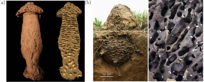
Les nids d’insectes et notamment ceux construits par les fourmis et les termites fas-cinent depuis longtemps les observateurs, biologistes, physiciens ou non scientifiques. Une première approche biologique de ces structures est l’approche fonctionnelle, qui cherche à comprendre l’adaptation des espèces à leur environnement et leur évolution au cours des âges (à l’échelle de temps de l’évolution de ces espèces). Une particularité des insectes sociaux est que certaines espèces vivent dans un nid qu’elles construisent elles-mêmes et c’est en grande partie grâce à ce nid qu’elles s’adaptent à l’environnement, car le nid assure le maintien d’un micro-environnement et de conditions climatiques favorables. L’approche fonctionnelle a montré que les constructions des insectes sociaux constituent des structures dynamiques dont l’organisation peut être d’une grande complexité [1, 2] et qu’elles ont des architectures très diversifiées avec des propriétés intéressantes en termes de réseaux de communication [3], de réponse aux perturbations, de ventilation et de climatisation [4, 5, 6]. Les figures 1.1, 1.2 et 1.3 présentent plusieurs exemples de nids de différentes espèces de termites et de fourmis. On peut notamment observer dans ces structures une organisation étagée, avec des chambres de formes très différentes selon les espèces (voire pour une même espèce selon les conditions extérieures), interconnectées par des tunnels et des passages reliant les étages adjacents. Ces derniers peuvent prendre la forme d’escaliers en colimaçon, qui constituent une des structures les plus complexes réalisée collectivement par des animaux vivant en société.

Il existe une deuxième approche de ces structures, qui s’intéresse aux mécanismes impli-qués dans leur morphogenèse. Ce qui est étonnant est, qu’aussi imposantes que ces structures puissent être, elles sont produites par des insectes dont la taille peut parfois être de plusieurs ordres de grandeur plus petite, dont les capacités cognitives sont très limitées comparées aux nôtres et qui peuvent pour certaines d’entre elles être quasiment aveugles. L’idée que

(a) (b)

Figure 1.1: Nids construits par des termites (1). (a) Nid de termites Cubitermes (photo et coupe reconstruite par tomographie aux rayons X). On observe une organisation en plusieurs étages. (b) Nid semi-souterrain de termites Cornitermes cumulans (Brésil) construit à partir de particules de terre et de matériaux organiques (vue extérieure et intérieure). On peut distinguer des chambres connectées entre elles par des tunnels.

la complexité et la diversité des nids puissent émerger de la combinaison de comportements individuels simples de chaque insecte a été énoncée en 1957 par Grassé [8] et vingt ans plus tard Deneubourg [9] propose pour la première fois d’utiliser la notion de processus d’auto-organisation pour expliquer certaines étapes de la construction du nid chez les ter-mites : selon cette idée, ces structures ne sont pas construites selon un plan préexistant ou selon les ordres d’un individu jouant le rôle d’“architecte” en cordonnant les actions de tous les autres individus mais elles émergent de l’interaction d’un grand nombre d’actes de construction simples effectués par des individus qui agissent chacun uniquement sur la base d’informations locales. Cette hypothèse a inspirée de nombreux travaux de modélisation qui ont d’abord concerné la construction de plusieurs parties emblématiques de ces structures (la chambre royale, les piliers, etc. [10, 11]). Ces travaux ont permis de reproduire des observa-tions telles que la transformation d’un pilier en un mur ou l’adaptation des dimensions de la chambre royale à la taille de la reine en utilisant des modèles contenant des comportements individuels réalistes (mais non validés et quantifiés expérimentalement). L’identification et la modélisation des comportements individuels impliqués dans la construction à partir de données expérimentales quantitatives et leur validation par des données expérimentales au niveau de la structure produite fait l’objet d’études plus récentes [12, 13, 14, 15, 16]. Toute-fois cette approche est encore peu développée et la compréhension détaillée des mécanismes

(a)

(b)

(c)

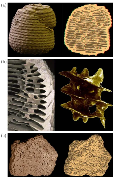
Figure 1.2: Nids construits par des termites (2). (a-b) Nid souterrain de termites Apico-termes. Ce nid comporte des structures ressemblant à un escalier en colimaçon permettant le passage entre deux niveaux. (c) Fragment de mur (souterrain) d’un nid de termites Sphae-rotermes sphaerothorax.

Figure 1.3: Nids construits par des fourmis. (a) Nid de fourmis Lasius fuliginosus construit en pâte de bois. (b) Nid de fourmis Lasius pallitarsis c Alex Wild. On distingue plusieurs étages. (c) Détail d’un nid de Lasius niger. Ce nid comporte des structures ressemblant aux escaliers en colimaçon des termites Apicotermes. Ces figures sont tirées de [7].

(a) (b)

Figure 1.4: Structures construites en laboratoire (équipe DYNACTOM) par des fourmis Lasius niger dans une arène de diamètre 10 cm. (a) Photo prise au bout de deux semaines. (b) Dynamique temporelle de la croissance du nid observé à l’aide d’un scanner de surface. Ces expériences ont pour objectif d’étudier la première phase de construction du nid. On distingue d’abord l’émergence de piliers puis d’arches qui relient des piliers voisins et sont les précurseurs de plafonds et donc d’une construction à plusieurs étages.

impliqués dans la construction de nids reste aujourd’hui une question largement ouverte. La présente thèse s’inscrit précisément dans cette problématique. Elle a bénéficié d’une collaboration entre deux groupes de recherche toulousains, l’équipe DYNACTOM au sein du laboratoire CRCA et l’équipe GREPHE au sein du laboratoire LAPLACE, le premier étant spécialisé dans l’étude des comportements collectifs dans les sociétés animales et le second étant spécialisé dans l’étude de la physique des systèmes complexes hors d’équilibre, depuis la physique des plasmas jusqu’à la thermique des transitions de phase liquide-vapeur ou la dynamique climatique des atmosphères planétaires. Malgré leurs domaines d’application initialement très distincts, ces deux équipes ont toujours partagé un intérêt commun pour l’étude détaillée des passages d’échelle, depuis l’individu dans un cas ou la particule/molécule dans l’autre, jusqu’à un système d’extension nettement supérieure ne portant plus de trace explicite des mécanismes élémentaires dont il est pourtant le résultat. Un autre point com-mun, plus méthodologique, est le choix de ces deux équipes d’aborder cette question non pas uniquement d’un point de vue théorique mais systématiquement en relation avec des travaux expérimentaux. Cette collaboration a été initiée à l’occasion d’un projet concernant la construction chez les termites [11]. Elle a ensuite été approfondie au travers de plusieurs études du phénomène d’agrégation de cadavres chez les fourmis Messor Sancta [17, 18, 19]. Ce phénomène d’agrégation particulier s’est avéré très riche et son étude a été poursuivie de manière continue jusqu’à aujourd’hui, même si elle a été parfois reléguée au second plan derrière d’autres projets communs concernant notamment le déplacement et l’agrégation de blattes ainsi que les bancs de poissons. Aujourd’hui, l’agrégation de cadavres revient au centre des préoccupations du fait de l’implication croissante de l’équipe DYNACTOM dans des études concernant la construction chez les fourmis et les termites.

Nous avons ici fait le choix d’aborder le problème de la modélisation des comportements individuels impliqués dans le processus de construction chez les insectes sociaux en identifiant quelques “grandes questions” auxquelles on se retrouve systématiquement confronté dans ce contexte et de travailler ces questions sur un terrain mieux maîtrisé, celui de l’agrégation de cadavres. Parmi ces grandes questions, il y en a d’abord deux qui sont la question de l’interaction entre le déplacement des insectes et la dynamique de la structure (principalement l’effet de la structure sur le déplacement) et la question de l’interaction entre les actes de prise et dépôt des matériaux de construction et l’environnement (notamment l’écoulement d’air, modifié par les structures produites, qui peut moduler les propensions à prendre et/ou déposer). Suivent un ensemble de questions méthodologiques en lien avec les contraintes d’une modélisation au contact de l’expérimental et pleinement inscrite dans le champ disciplinaire de l’éthologie, visant notamment à tester et enrichir les connaissances actuelles sur les boucles

sensori-motrices ou plus largement les actes comportementaux individuels impliqués dans la construction.

La première question concerne l’interaction entre le déplacement des insectes et la dy-namique de la structure que ces insectes sont en train de construire. Quel est l’effet de ces interactions sur les dynamiques de construction et comment les modéliser ? D’une part, le déplacement des insectes détermine le transport du matériau de construction et agit donc sur la structure construite. D’autre part, la structure agit en retour sur les trajectoires des insectes. L’existence de cette rétroaction de la structure sur le déplacement est évidente dans le cas des nids où les constructions comportent des murs ou des piliers infranchissables mais l’effet de la structure sur le déplacement a aussi été démontrée dans le contexte de l’agréga-tion de cadavres, où les fourmis ont tendance à suivre les bords des tas de cadavres [18, 20] (même s’il ne s’agit pas d’obstacles infranchissables dans ce cas). Les différentes tentatives de modélisation du phénomène d’agrégation de cadavres ont de plus montré que ce phéno-mène de suivi de bord est de première importance : son étude est nécessaire si l’on souhaite comprendre la dynamique des tailles des structures produites en champ bi-dimensionnel [21]. La deuxième question, le couplage entre les comportements individuels et les facteurs environnementaux (courants d’air, température, humidité) est essentielle si l’on souhaite comprendre les mécanismes d’adaptation des nids aux conditions environnementales. En effet ces nids semblent disposer de systèmes passifs de ventilation et de conditionnement d’air (température, hygrométrie, concentration en CO2, etc. [4, 6, 1, 2]). Comment modéliser ces

couplages ? Ces couplages existent aussi dans l’agrégation de cadavres où il a été montré qu’un écoulement d’air de faible vitesse modifie significativement les dynamiques d’agrégation de cadavres.

La troisième famille de questions, les questions méthodologiques, a été abordée tout au long du travail pratique sur les deux premières. Nous avons été constamment confronté à des difficultés relevant de la démarche de modélisation (impossibilité d’observer directement les comportements individuels, nombre restreint de données expérimentales disponibles pour l’inversion de ces comportements à partir d’expériences faisant intervenir plusieurs de ces comportements de façon couplée, pertinence biologique des propositions comportementales étant donné les connaissances disponibles concernant les capacités perceptives et motrices des individus, etc.). A chaque fois qu’une telle question surgissait, nous l’avons utilisé pour tenter de clarifier les fondements de notre pratique. Nous nous sommes pour cela beaucoup appuyé sur l’histoire d’une dizaine d’années de travail sur l’agrégation de cadavres en champ mono-dimensionnel (le long du bord d’une arène circulaire). Le résultat de ces réflexions est l’article constituant le Chap. 2. Le choix de le présenter au début de ce manuscrit de thèse

(bien que les réflexions sur la démarche de modélisation ne soient pas le point de départ mais plutôt le résultat du travail présenté dans les deux autres chapitres) a pour but de permettre au lecteur de percevoir l’ensemble de ces enjeux lors de sa lecture des analyses expérimentales et des propositions de modèles que nous présentons dans le cadre de l’étude du déplacement et de la construction.

Bien sûr tous les ingrédients de la construction ne sont pas présents dans l’agrégation de cadavres sur laquelle nous nous sommes concentrés. Par exemple, dans la construction, les insectes ajoutent une substance chimique aux boulettes de matériau de construction avant de les coller dans la structure. Une fois collées, ces boulettes sèchent au cours du temps ce qui les rend de plus en plus en difficile à arracher. La probabilité qu’une boulette collée soit reprise par un insecte décroît alors au cours du temps. Un tel mécanisme, qui ajoute de la complexité au modèle, n’existe pas dans notre cas. C’est un choix que nous faisons de nous concentrer sur un ensemble de questions restreintes dans un cadre mieux maîtrisé, mais ce choix ne prend son sens que du fait de l’ensemble des travaux initiés en amont et en parallèle de cette thèse. Il s’agit d’une part de travaux concernant l’identification et la quantifica-tion des comportements individuels impliqués dans la première phase de la construcquantifica-tion du nid chez la fourmi Lasius niger et chez le termite sud-américain Cornitermes cumu-lans, avec comme premières étapes la conception de protocoles expérimentaux permettant de reproduire le processus de construction dans des conditions contrôlées et l’exploration qualitative de règles comportementales susceptibles d’expliquer les structures construites [7]. Par exemple la Fig. 1.4 montre une structure construite par des fourmis Lasius niger dans le cadre d’expériences réalisées dans l’équipe DYNACTOM. D’autre part, un ensemble de travaux visent à caractériser les structures produites par les fourmis et les termites. Un pre-mier objectif de ces travaux est la constitution d’une base de données contenant les images tri-dimensionnelles de nids de fourmis et de termites récoltés dans la nature en utilisant no-tamment la tomographie aux rayons X. Un deuxième objectif est de s’appuyer sur ces images pour caractériser l’architecture des nids : Dans certains cas, il est possible de décrire l’or-ganisation spatiale des structures observées en termes d’éléments architecturaux comme des tunnels ou des chambres (notamment pour les nids du genre Cubitermes [3]) ce qui permet ensuite de réaliser une analyse topologique (connexions existants entre les différentes parties du nid et avec le milieu extérieur, longueur moyenne des trajets entre différentes parties du nid, etc.) et de tenter une interprétation en termes fonctionnels (par exemple l’efficacité de circulation interne ou de défense contre les prédateurs).

En revenant à notre sujet d’études, on peut noter que beaucoup d’insectes sociaux, et no-tamment une multitude d’espèces de fourmis, agrègent différents types d’objets : il peut par

exemple s’agir de leurs larves [22], de graines [23, 24], de fragments de feuilles [25], de grains de sable [13] ou bien de boulettes de terre comme dans les premières phases de construction. Ici nous considérons le cas particulier des fourmis Messor Sancta qui, en conditions natu-relles, vivent dans des nids souterrains. Lorsque des fourmis meurent dans la colonie, leurs congénères les transportent en dehors du nid et regroupent les cadavres sur des tas. L’intérêt de ce phénomène dans notre contexte est la possibilité de le reproduire en laboratoire dans des conditions contrôlées (voir notamment [26, 17]). Il est alors possible de maîtriser les pa-ramètre extérieurs influençant le processus d’agrégation (le nombre de fourmis en présence, la température, l’hygrométrie de l’air, les courants d’air, etc.). Dans les expériences réali-sées par Theraulaz et coll. [17], les cadavres sont initialement disposés le long du mur d’une arène circulaire. Ensuite les fourmis accèdent à l’arène. Au cours des expériences les fourmis se déplacent dans l’arène, prenant des cadavres à certains endroits et les déposant ailleurs. Comme la fourmi Messor Sancta a une forte tendance à suivre les bords de l’arène (ce com-portement, appelé thigmotactisme, a été étudié par Casellas et coll. [20]), toute l’expérience a lieu dans une petite bande le long du mur de l’arène. Les cadavres sont d’abord regroupés dans des zones assez nombreuses et étalées. Ces zones sont ensuite ramassées de façon plus dense et les petites zones disparaissent au profit des plus grandes. Après une dizaine d’heures on observe un petit nombre de tas très denses et stables. Nous avons déjà mentionné que cette configuration mono-dimensionnelle a été largement étudiée au sein de nos deux équipes et la raison en est que ce dispositif facilite grandement le travail de modélisation. Les diffi-cultés posées par la compréhension des mêmes mécanismes en champ bi-dimensionnel sont clairement beaucoup plus élevées. Elles ont été largement abordées dans le cadre d’une pre-mière thèse au sein de l’équipe DYNACTOM [18] (voir aussi [19]) et nous bénéficions ici directement des données expérimentales correspondantes. Dans ces expériences les cadavres sont initialement disposés de façon aléatoire sur toute la surface de l’arène et on peut ainsi observer l’émergence de tas de cadavres loin des bords. Lorsque les expériences sont réalisées en présence d’un courant d’air de faible vitesse (trop faible pour déplacer directement les cadavres), ces tas sont allongés dans la direction du courant et se déplacent dans le sens de celui-ci.

Comme nous l’avons déjà mentionné, la thèse s’ouvre sur un chapitre méthodologique (Chap. 2). Ce chapitre n’a aucune dimension bibliographique exhaustive. L’état de l’art et le positionnement de notre travail sur le déplacement par rapport à la littérature la plus proche sont reportés au début du Chap. 3 présentant notre proposition de modèle du phénomène de suivi de bord, qui est de ce fait le plus long de la thèse. Dans le Chap. 4 nous nous appuyons sur les précédents chapitres pour proposer un modèle complet de l’agrégation de cadavres, dans lequel l’influence des structures sur le déplacement tient une place centrale.

Ce chapitre traite aussi de l’interaction du processus d’agrégation avec un écoulement d’air de faible vitesse. La discussion finale du Chap. 5 sera l’occasion de replacer le phénomène d’agrégation de cadavres dans la perspective plus large de l’analyse de la construction et d’es-quisser les perspectives de travaux futurs. Dans la littérature concernant l’effet de structures solides sur le déplacement des insectes, et notamment le suivi de ces structures, le concept comportemental le plus communément mentionné est celui de thigmotactisme. Nous verrons très rapidement au début du Chap. 3 que ce concept, désignant un phénomène d’orientation (taxis) par contact tactile (thigma) ce qui suggère un alignement des insectes avec le bord (maintien d’un contact antennaire), est loin d’être le seul permettant d’interpréter ce type de suivi et par la suite le modèle que nous mettrons en avant, qui appartient à la famille des klinotaxies, ne conduit pas à un tel alignement. Pour autant nous maintenons le mot de thigmotactisme dans l’intitulé de notre travail de façon à faire une référence explicite aux travaux précédents.

Considérations méthodologiques

Modeling of collective animal behaviors in a cognitive

perspective : a methodological framework

Sebastian Weitz1,2,∗_{, St´ephane Blanco}1,2_{, Richard Fournier}1,2_{, Jacques Gautrais}3,4_{, Christian Jost}3,4

and Guy Theraulaz3,4

1_{Laboratoire Plasma et Conversion d’Energie, UMR-CNRS 5213, Universit´e Paul Sabatier, Bˆat 3R1,}

118 Route de Narbonne, F-31062 Toulouse cedex 9, France

2_{CNRS, Laboratoire Plasma et Conversion d’Energie, F-31062 Toulouse cedex 9, France}

3_{Centre de Recherches sur la Cognition Animale, UMR-CNRS 5169, Universit´e Paul Sabatier, Bˆat}

4R3, 118 Route de Narbonne, F-31062 Toulouse cedex 9, France

4_{CNRS, Centre de Recherches sur la Cognition Animale, F-31062 Toulouse cedex 9, France} ∗_{Corresponding author: [email protected]}

1

Introduction

Collective animal behaviors have generated an increasing number of studies over the past decade [1–3]. These phenomena can be observed at all living scales, from bacteria colonies [4] to bird flocks [5], fish schools [6, 7], insect societies [8, 9] or herds of gregarious vertebrates [10, 11]. These collective behaviors are typically governed by self-organized processes resulting from many direct or stigmergic interactions between individuals and they generally lead to the formation of dynamical patterns whose temporal and spatial characteristic lengths are much larger than the typical range of interactions [12–14]. Understanding how interactions between individuals control collective behaviors is a challenging problem for a growing research community in biology and statistical physics [15]. Indeed this is a required condition to establish a continuous causal link from studies dealing with the neurophysiological or cognitive basis of individual behavior and studies dealing with collective behaviors in which these neuronal or cognitive processes are involved (e.g. [16,17]). Moreover, understanding interactions allows the prediction of collective behaviors in different conditions and the identification of key variables, thus opening the way to the control of collective behaviors [18].

Addressing these interactions starts with the enunciation of presumed sets of behavioral rules that are inspired by and confronted to experimental observations. These sets of rules that define the suggested behavioral model are most commonly of statistical nature: Individual behavioral mechanisms are

char-acterized by the individual’s probabilities to perform a given action (e.g. changing its own direction of motion in a given time interval) or their probabilities to undergo a transition from a state A to a state B [19–21], many of them depending on external stimuli (e.g. information about conspecifics and environ-ment). In methodological terms, a very demanding task is that of maintaining as sharp a distinction as possible between the behavioral model, enunciated as a given combination of biological concepts, and its formal translation that may not be unique as it depends on the retained set of quantitative state variables and involves adjustable functional dependences for each statistical response to stimuli. Only when this distinction is made can the model be criticized for its biological pertinence and the formal translation for its rigor. In this sense, establishing that the model is compatible with the corpus of knowledge in neurosciences, animal cognition and behavior and with available observational data is one issue; using observational data to adjust the functional dependences is quite a different one, although both issues are commonly addressed using the very same statistical techniques as far as observational data are concerned. Historically, the second issue was left aside in a first approach to the understanding of the mechanisms underlying collective phenomena. The objective was to demonstrate that the diversity and complexity of the behavioral patterns observed in swarms, flocks, schools and crowds may result from relatively simple interactions between the individuals [2,22,23]. It was therefore sufficient to enunciate biologically meaningful behavioral models and check, using numerical simulations, that these behaviors lead to the emergence of dynamical patterns qualitatively similar to the addressed ones [10,24–26]. This first step was essential as a justification of the forthcoming long term researches toward more quantitative assessments. It has permitted, in particular, to test alternative hypotheses about the behavioral mechanisms taking part in a given collective behavior. But one of the essential conclusions was also that very different individual mechanisms may reproduce similar collective phenomena. For instance, [27] and [28] have both proposed models for the clustering of objects by ants moving at random in a two-dimensional space. In both models an unloaded ant encountering an object on its path picks it up with a probability pp.

In [27] pp depends on the number of objects encountered during a given preceding time interval (which

is a rough indication of the object density in the neighborhood), whereas in [28] unloaded ants pick up every object encountered (pp= 1). Despite this important difference, [28] highlights that the clustering

dynamics of both models are qualitatively the same and close to the experimental observations.

Although this first historical phase is far from being over (numerous qualitative or semi-quantitative studies are still today offering very useful conceptual contributions), an increasing number of recent

studies use quantitative approaches in which macroscopic quantities are measured at the group scale in order to characterize the collective dynamics. These measurements have permitted to carefully adjust the functional dependences so that the observed collective patterns are quantitatively reproduced [29–31]. These more detailed explorations have essentially confirmed the previous conclusions, in particular that with adequate adjustments, biologically different models at the individual scale are able to reproduce the same collective dynamics, even from a rigorously quantitative point of view.

A very strong consequence of such observations was to establish that it was biologically meaningful to think in terms of renormalization groups, universality classes and asymptotic theory for all studies concerning the dynamics of collective patterns (as was already established for macroscopic physics [32,33]). This led to numerous research efforts toward the identification of minimum behavioral models associated to some of the most challenging collective behaviors, in particular as far as fish schools and bird flocks are concerned [24,25,34]. However, in the context of theoretical biology, these efforts are only relevant to the understanding of the collective behavior itself, closing the door to the above mentioned neurophysiological and cognitive direct connections. Researchers dealing with minimum behavioral models do not claim that the considered animals actually follow minimal rules; they state that a given collective pattern dynamics is best described with a behavioral model that may serve as a reference for all analyses at the collective scale. The parameters of these reference models may then be defined as effective parameters that are related to neuronal and cognition details. But how they are related is not an issue : two distinct sets of individual behavioral rules leading to the same effective parameters are indeed the very same model at the collective scale. From this point of view, the fact that we observe it to be impossible to discriminate between them by collective measurements is a methodological validation and nothing like a practical difficulty.

Researchers equally involved in the understanding of collective dynamics in animals may as well conclude from the same facts that further observational data are required as soon as they are interested in the analysis of individual behaviors at the level of details of neuronal and cognitive processes for a particular species in a given (ecological) context. However, choosing an adequate experimental protocol to decipher between alternative models often proves to be a very difficult task. For instance, a model of the formation of the dominance order in social wasps based on threshold reinforcement has first been experimentally verified from dominance behaviors measured at the individual scale [35, 36]. However, some years later, the same authors questioned the occurrence of this reinforcement mechanism because

the empirical data may as well be explained by preexisting differences among individuals [37], so the available experimental data were not discriminative, even at the individual scale.

All this illustrates that we are still today at the stage of methodological reflections and regularly have to go back to quite basic questions: When attempting to identify physiologically validated components of the individual behavior, what are the respective roles of collective observational data and more specific experimental protocols in terms of model validation and function / parameter estimation? Are there criteria that can guide the design of an experimental protocol? The aim of this paper is to address these questions in the particular case where laboratory experiments can be designed providing observational data that are fully independent of the initial collective observations. This means that we leave aside the more difficult question of designing individual observation protocols based on the very same experiments (or field observations) as those allowing collective quantitative measurements. We start in Sec. 2 from a published experimental study on object clustering. Six different individual behavioral models are con-structed, with rules in terms of statistical responses to the relevant stimuli, that all reproduce satisfyingly the collective patterns. It is then theoretically established that two of these models, although they are clearly distinct in terms of individual behaviors, cannot be discriminated using collective scale observa-tional data, whatever their accuracy and amount. Section 3 then addresses the methodological questions associated to the design of additional individual-based experimental protocols, as well as the use of the corresponding data for model validation and inversion of free parameters. A sequence of methodological steps is proposed and practically illustrated using the same object clustering example as in Sec. 2 and the expected benefits are discussed in Sec. 4.

2

Identical collective pattern dynamics with distinct individual

behaviors

We will tackle all methodological issues with the help of a simple example of collective animal behavior: object clustering in the ant Messor Sancta [38] (see Fig. 1). In this example, the objects clustered by the ants are corpses of their dead conspecifics1_{. The clustering process has been shown to be}

self-organized [38]. The spatial structures result from complex dynamics in which the behavior of each ant is 1_{Note that social insects, and in particular ants, are also known to build clusters of many other kinds of objects (e.g.} brood [39], seeds [40, 41], sand pellets [42] and leaves fragments [43]).

indirectly influenced by the product of the activity of its conspecifics. One of the features of this collective phenomenon is that the behaviors can be studied under controlled laboratory conditions at two different scales, that of an individual and that of the resulting aggregates. The experiments reported in [38] were carried out in circular arenas (see Fig. 1-A). To prevent the use of external cues, the whole set-up was surrounded by white tissue, which also ensured an indirect and diffuse lighting. As the objects (the ant corpses) are initially distributed homogeneously along the arena wall and as the ants exhibit a strong tendency to follow the inner wall of the arena as a consequence of their thigmotactic behavior, the whole clustering process takes place within a small band along these walls. When the ants are given access to the arena, the colony being placed beneath the experimental arena and ants entering through the central hole, they move along the walls, pick up objects at some places and drop them elsewhere. After a few hours several small piles, regularly distributed in space, can be observed. The bigger piles grow at the expense of the smaller ones, that have completely disappeared by the end of the experiment (see Fig. 1-B). Therefore the measured mean number of piles (see Fig. 1-C and Fig. 1-D) rises first up to a peak after ca. 2h hours (about 11 and 25 piles, respectively, for the small and high object density configurations), then decreases and finally reaches a quasi-stationary number at the end of the experiment (after 50 hours, about 3 and 4-5 piles, respectively).

The purpose of a biological enquiry upon such clustering dynamics is to formulate and validate an individual behavioral model which could explain it. If we decide to start with the simplifying assumption that no significant chemical marking process involving a pheromone deposition is at work and that direct interactions between individuals (e.g. collisions) play a neglectable role, then the most conservative model for how ants move is a diffusive random walk. The two other relevant individual behaviors a model should account for are then how and when ants decide picking up and dropping objects. For the aggregation process to occur, we basically have to consider that ants will react somehow to the distribution of objects, i.e. they must be reactive to the local density of objects. We assume that this information may be summarized by η = N

S, where N is the number of objects in the perception area S around the

ant. This stimulus will be referred to as the perceived object density. Under the assumption that no other stimulus is significant, clustering can only occur if the perceived object density favors dropping (“Dropping stimulated by η”) or inhibits picking up (“Picking up inhibited by η”), or both. These sensitivities are indeed required to amplify density fluctuations and compete against the homogenizing potential of the diffusive random walk.

0 10 20 30 40 50 0 2 4 6 8 10 12 14 time (h) n umber of piles C low density 0 10 20 30 40 50 0 5 10 15 20 25 30 35 time (h) n umber of piles D high density

Figure 1. Clustering experiments. Objects are uniformly distributed along the border of a 50 cm diameter circular arena. Two different initial one-dimensional densities are used: 127 and 255 objects per meter. The duration of each experiment is 50 hours. Fig. A and Fig. B correspond respectively to the beginning and the end of a high density experiment. Fig. C and Fig. D display the time series of the number of piles (mean ± s.d.) for the low and the high density experiments, respectively. Piles are defined as follows: Two neighboring objects are considered to belong to the same cluster if the distance between them is less than 1 mm. A cluster constitutes a pile if it contains at least 6 objects. In [38] another circular arena with a 25 cm diameter was also used (with the same low and high initial densities). For the purpose of the methodological illustration of Sec. 2 only the large arena is used, but the model built in Sec. 3 is compatible with all observations, including the ones in small arenas.

However, quite distinct hypothesis can still be made for questioning the biological meaning of what happens. For the purpose of a brief illustration, we will play in this section with three behavioral concepts: we will question the influence of the perceived object density, the importance of inter-individual variability, and the role of individual temporal correlation.

The influence of the perceived object density targets the shape of the stimulus-response function, namely what the ants react to. As far as corpses are concerned, Anderson [44] explicitly asked: “But what if an ant regards a group of two or more ants as a processed pile and perceives a single dead ant as something qualitatively different—perhaps as an unprocessed ant that just happened to die on that spot?”. It is generally admitted that dropping behavior is favored by the local objects density, but does it also affect the picking up behavior? In such a contextual frame, the model interpretation would be about whether there is some distinct information processing dedicated to objects perception or not. Object density could well favor local dropping simply due to mechanical constraints because it is harder to carry an object through an aggregate of objects. It is known for instance that ants can build walls of rocks by just reacting to obstacles [28] or mounds by randomly dropping their load [45], in which case there is little need for sophisticated cognitive processes. Yet, some other species display an added complexity for nest wall building, with individuals coordinating the choices of material they fetch on independent forays [46].

The inter-individual variability would refer to different activity levels among workers, which is well-known in social insects as division of labor [47,48]. Division of labor and task partitioning in social insects are often cited as major features of their ecological success as they are reputed to increase colony efficiency because specialized workers can become superior in performance for their task [49–51] although this is controversial [52]. In the context of necrophoric behavior, it can also allow the colony to keep waste-workers and waste piles away from vital resources (e.g. fungus garden) so as to reduce contamination risks [53,54]. The division of labor can stem from genetic basis [55,56] but is strongly adaptive to colony size and needs as well as to workers’ age [48, 57, 58] and physiological state [59]. Such differentiated objects handling activity was introduced in the model by assuming inter-individual variability, i.e. their picking up and dropping statistics depend on an activity level a that is constant in time but differs for each ant. The activity level could for instance be related to age or any kind of genetic and epigenetic factors. Inter-individual variability could play a significant role if the activity level distribution is wide enough for picking up and dropping to depart from a population with all individuals reacting the same.

Finally, individual temporal correlation refers to some kind of memory effect, i.e. the behavioral decision (e.g. dropping) is affected by the time elapsed since the last behavioral decision (e.g. picking-up). Such reference to a memory effect has been recently suggested for the necrophoric behavior in Myrmica rubia [60]. A memoruless behavior would not exhibit temporal correlation, i.e. the behavioral response at time t would only depend on what is perceived by the ant at that time, and this is generally assumed implicitly in behavioral models based on stimulus-response functions. Note that such a memoryless model would not exclude learning processes or individual experience for specialized individuals [61, 62] as they could still be accounted for by adapting the parameters of the stimulus-response function itself. However, since we are interested only in memory effects of the same magnitude as the time scale of the collective phenomenon, we rather chose to test a true memory effect modelled by a decreasing propensity to pick-up or drop as the time elapses: the longer the time an ant has been carrying a object, the less reactive it will be to local density, as if it would explore longer for a higher density to compensate for the increasing effort made to reach it.

Table 1 summarizes how these three behavioral components are combined to produce six different models. All the corresponding quantitative details, as well as the illustration of the functional adjustments are provided in the Appendix. The point is that all six models allow functional adjustments which make them quantitatively compatible with the available data on clustering dynamics (cf. 2), although they strongly differ in terms of cognitive implications as far as the interpretation of picking up and dropping behaviors are concerned.

At this stage, further investigations to identify the most relevant individual model would certainly start by looking for more detailed quantitative measurements on the basis of the same observed clustering dynamic. In addition to the temporal evolution of the number of piles, one may analyze the distribution of inter-aggregate distances, of aggregate sizes (number of aggregated objects), aggregate dimensions, etc., hoping that these distributions could be characterized with enough statistical accuracy to exclude some of the six models. However, one may easily think of numerous cases in which the required accuracy would be so high that no experimental protocol would allow it to be reached. It is for instance impossible, from macroscopic observations of gaseous properties, to discriminate between two molecules having different collision cross-sections if these different “interaction behaviors” lead to the same values of viscosity and conductivity. But in our illustration example this point can be made even more clearly than the way the asymptotic theory, which requires that a clear definition of the macroscopic limit is accepted, does

it: we proved indeed theoretically that it is strictly impossible to discriminate between models 3 and 5, or between models 4 and 6, whatever the amount and the accuracy of the information acquired from the observed object displacements, in particular whatever the observation scale. The extended proof is given in the Appendix, but its principle is quite simple:

• The picking up probability is the same for each individual ant in models 5 and 6, whereas it depends on the activity level in models 3 and 4, but the activity level distributions are such that the population average value of the picking up probability of model 3 equals that of model 5, and that of model 4 equals that of model 6. Each object is therefore picked up with the same temporal statistics within each model pair.

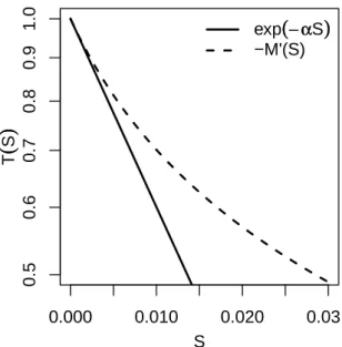
• The probability of still carrying an object decreases exponentially as function of time in model 3 and model 4, whereas it decreases non-exponentially in model 5 and model 6, but the survival curves in models 5 and 6 are such that, when the whole population is integrated, they lead to the same deposition statistics as those of models 3 and 4 respectively.

• For each object, the picking up and deposition statistics resulting of the whole population are there-fore rigorously identical within each model pair, which excludes that the models be discriminated by the observation of object displacements, whatever the accuracy level.

The conclusion would be the same even if the living ants could also be followed and their behavior statistically analyzed during the clustering experiments, provided that a single ant could not be tracked long enough for its individual statistics to be characterized independently of the other ants. Otherwise the activity level distribution could indeed be observed and models could be discriminated. The crucial alternative is therefore the access or not to the details of the individual ant behavior.

3

A methodological approach for the identification of individual

behavioral rules

The preceding examples were meant as an introduction to the methodological questions raised by the objective of not only modeling the collective dynamics, but also learning about the involved individual behaviors with enough details and confidence to allow fruitful contributions to cognitive and neural bi-ological research. The literature emphasizes the fact that details of the individual behaviors are widely

Table 1. Formulation of the six different models. The table indicates, for each model, the choices made in terms of inter-individual variability, temporal correlation, and picking up/dropping dependence on perceived density η. In each model, unloaded ants are assumed to be distributed uniformly along the border of the arena and their lineic density is constant in time. As it is further assumed that objects do not overlap, the uniformity of the unloaded ant distribution implies that all objects are encountered with the same rate and the picking up behavior is entirely characterized by the probability p(η) to pick up an encountered object as function of the perceived density η at the object location (p also depends on the activity level a, and is noted p(η, a), when inter-individual variability is accounted for). After picking up an object, the loaded ant moves according to a one-dimensional diffusive random walk (in all six models the constant walking speed along the arena’s border is v = 1.6 10−2 _{m· s}−1_{and the rate at}

which U-turns occur is 1

τU with τU = 9.9 s). The dropping statistics is entirely characterized by the

survival probability T (t) (the probability that the ant carries the object longer than t) that depends on the perceived density along the path, i.e. on η(t0_{) at each time t}0 _{in the [0, t] interval (T (t) also depends}

on a, and is denoted T (t, a), when inter-individual variability is accounted for). Inter-individual variability is characterized by the probability density function of the activity level f(a). All parameter values and detailed functional dependences are provided in the Appendix.

Inter-individual Temporal Picking up Dropping variability correlation inhibited by η stimulated by η

Model 1 NO NO NO YES

Model 2 NO NO YES YES

Model 3 YES NO NO YES

Model 4 YES NO YES YES

Model 5 NO YES NO YES

Model 6 NO YES YES YES

● ● ● ● ● ● ●●_●● ● ● ●●● ●_● ● ● ● ● ●●● ● ●●●● ●● ● ● ● ● ●●●● ● ●● ● ●●● ● ● ● ●●● 0 10 20 30 40 50 0 2 4 6 8 10 12 14 time (h) n umber of piles ● ● ● ● ● ● ●●_●● ● ● ●●● ●_● ● ● ● ● ●●● ● ●●●● ●● ● ● ● ● ●●●● ● ●● ● ●●● ● ● ● ●●● ● experimental model 1 model 2 models 3/5 models 4/6 A low density ● ● ● ● ● ● ● ●● ● ●_●● ● ●●●●● ●●●_●●●●●_●●●●●●●●●● ●_●●●● ●●●●● ● ●●●_● 0 10 20 30 40 50 0 5 10 15 20 25 30 35 time (h) n umber of piles ● ● ● ● ● ● ● ●● ● ●_●● ● ●●●●● ●●●_●●●●●_●●●●●●●●●● ●_●●●● ●●●●● ● ●●●_● ● experimental model 1 model 2 models 3/5 models 4/6 B high density

Figure 2. Clustering dynamics of the six different models. Figures A and B indicate the time series of the number of piles for models 1-6 compared to the experimental data (mean ± s.d.) in the low and high density settings, respectively. The predictions of all the models are compatible with the experimental observations. Moreover, the predictions of model 5 are rigorously identical to those of model 3, and the predictions of model 6 are identical to those of model 4.

irrelevant to the understanding of numerous emerging collective behaviors, which legitimates that solid theoretical conclusions can be drawn without deep references to a physiological knowledge of the con-sidered species. But the same fact translates into strong practical difficulties as soon as “details”, from a collective point of view, may correspond to such significant biological differences as with or without inter-individual variability and with or without short time memory usage. We even formally established the existence of configurations that rigorously exclude the discrimination of two different biological in-terpretations from observations of emerging structures, whatever the temporal and spatial observation scales: the emergence statistics can be strictly identical with two behavioral models that are very dis-tinct in terms of cognitive implications. We therefore face the question of looking at other observables than those defined for the purpose of collective modeling, using the same available experimental data, or implementing new experimental protocols specifically designed for the purpose of individual behavior modeling.

First of all, it may be useful to note that the distinction is quite subtle. There is nothing like a pure collective scale reasoning on one side, versus pure individual scale reasoning on the other. The question still remains the understanding of the collective behavior, which means that

• we are only addressing the components of the individual behavior that impact the collective features, • the individual model is only fully validated when it can be shown that the corresponding perceptions

and actions are sufficient to reproduce the addressed collective patterns.

The only difference from a pure collective scale reasoning is that we try to add the argument that the identified individual behavior is not only sufficient to reproduce the collective dynamics, but that it is indeed at work in the considered species. There could be ways to fully distinguish individual studies from collective ones if it were established that collective modeling would systematically lead to the identification of effective parameters that would summarize the effects of a potentially wide diversity of possible individual features. Individual behavior modeling could therefore take the effective parameters as their unique basis and the question would only be to understand which one, among all possible behaviors, is responsible for the observed effective parameter value in the considered species. This would be a complete parallel with, for instance, gaseous kinetics where fluid dynamics deals, at the hydrodynamic limit (the collective scale), with the question of how effective parameters such as viscosity and conductivity impact the flow dynamics, whereas quantum molecular physics deals, separately, with the question of

how specific molecular structures and properties give rise to the observed viscosity and conductivity values. This may appear to be meaningful as far as bird flocks and fish schools are concerned, but the preceding object aggregation examples are sufficient to demonstrate that individual models that are undistinguishable at the collective scale do not systematically refer to identical effective parameters in a common collective model. A strict separation between individual and collective studies is therefore hard to maintain.

Altogether: i) we need to go further than designing a valid collective model; ii) the additionally required information may not be accessible from collective observables; iii) the collective experimental data remain the material used for the final validation of the proposed individual model. At this stage, two approaches can be retained or combined: either the same experimental protocol (or field observations) are used and new observables are defined with the objective of closely characterizing the individual properties, or independent protocols are designed. We concentrate hereafter on the design of independent protocols, which may be considered as the easier approach (when possible) in the sense that: i) there is no ambiguity associated to the fact that the same data are used both for parametric quantification of the retained individual model and for final validation in terms of emerging collective features; ii) the involved different behavioral components can be addressed separately by designing experimental protocols dedicated to the characterization of a single component. We can think for instance of separate dedicated protocols for the movement of ants, for picking up and for dropping, whereas the initial object aggregation experiments involve the three actions simultaneously. We argue hereafter that when designing these protocols, strong benefits can be expected from the effort of distinguishing the following successive methodological steps:

1. enunciation of a behavioral model (or several alternative ones);

2. model translation into fully quantitative terms involving the choice of well defined state variables and stimuli;

3. validation and parametric inversion of the behavioral components that can be characterized inde-pendently of all other components, or one by one in an adequate sequence;

4. coupled validation and parametric inversion of the remaining components; 5. confrontation of model predictions to the available collective observational data.

Model enunciation The qualitative discussion of the behavioral model is the step at which most of the cognitive reasoning takes place. The term model is therefore to be understood as an argued cognitive representation of the individual as far as its influence on the collective dynamics is concerned. We will come back to this point in the discussion section, in particular to the fact that experimental protocols aiming at the detailed characterization of individual behaviors are designed with the idea of validating or invalidating one or several alternative behavioral models, and that a full explicitation of such initial orientations helps clarifying the following cognitive and physiological debates. Here we only illustrate this first step with the example of [38]2_{in which a literature review and preliminary experimental explorations}

led to the following model enunciation:

• Individuals have identical behaviors (no inter-individual variability).

• Direct inter-individual interactions play no role in the object aggregation process.

• Indirect inter-individual interactions by way of pheromone deposition play no role in the object aggregation process.

• Ants are always moving, speed changes play no role in in the object aggregation process and actions such as direction changes, picking up and dropping are instantaneous.

• Thigmotactism is so strong that ants remain strictly in a narrow band close to the arena border. • Objects never overlap.

• Objects are only perceived in the immediate vicinity of the ant, and this perception corresponds to an antenna contact and/or a visual perception, both having similar ranges (of the order of a few millimeters).

• In cognitive terms, object perception leads to the estimation of the local object density via an indirect measure of the number of objects in the perception area.

• Although object perception is very local, it could be claimed that the individual has access to more complete information concerning the object field if it kept a memory of the objects it encountered along its trajectory: the retained model states that such a memorization process is not at work and that, at each instant, the ant behavior is only influenced by local perception.

2_{Some of the illustrations corresponding to the work reported in [38] do not appear explicitly in the four pages format} of this article, but are all extracted from the broader, partially unpublished, underlying investigations.

Quantitative translation Complete model translation into quantitative terms requires arbitrary choices to be made for state variables and stimuli that cannot be deduced as direct consequences of the model once it has been enunciated. Arbitrary refers here to cognitive reasoning: if there were cognitive motivations for the quantitative definition of some state variables and stimuli, they should be part of the model itself and should be enunciated and justified in the preceding step. This does not exclude motivated arguments toward the choice of a given state variable (or stimulus) rather than another meaningful one, in partic-ular for practical reasons related to experimental observation or to any forthcoming formal derivation. Our object aggregation example provides various illustrations of the typical meanings of such required arbitrary choices. Quantitative translation of ants movement is the simplest of these illustrations: the only enunciated related properties are that ants remain close to the circular arena border, that speed changes are insignificant, and that direction changes are instantaneous, which is translated into the fact that ant locations are reduced to a lineic abscissa along the arena perimeter and that ant velocity is either clockwise or counterclockwise oriented, with a constant speed. This means in particular that the details of the thigmotactic behavior are left aside and that only its overall effects are quantified. Experimentally speaking, further detailed definitions were required in order to measure the abscissa and the orientation of each ant. A first ant location was identified using the center of the head and was projected on the perimeter; the orientation of the movement was then defined using the difference between the successive abscissa values corresponding to two successive frames, etc.; but this belongs to the measurement protocol and not to the model translation itself. More subtle but very well established is the translation of the fact that ants do not use any memorization process for the considered actions. We already mentioned the quantitative translation of this assumption in the preceding section when describing the model examples in which the assumption was made that no temporal correlation occurred. The fact that the enunci-ated model excludes any significant effect of memorization, combined with the assumption that direction changes, picking up and dropping are instantaneous, translates indeed into the statistical property that whatever occurs after a given time t is statistically uncorrelated to any preceding action or perception. This allows markovian formulations to be used, which leads in the present case to exponential survival probabilities such as those of Tab. 1 for the states of traveling clockwise, traveling counterclockwise and carrying an object. Practically speaking, this means that the actions of changing direction and dropping an object are fully quantitatively described by two functions of the object perception stimulus η: the di-rection change frequency νc(η) and the dropping frequency νd(η), or alternatively the average time before

direction change (the direction change mean free time) τc(η) = _νc1_(η) and the average time before dropping

(the dropping mean free time) τd(η) = _νd1_(η). An essential point is here that no arbitrary choice was made

for this translation: frequencies can be preferred to mean free times or vice versa, but the translation of a memoryless behavior with instantaneous actions is fundamentally unique, whereas the level of detail that was retained for the quantitative representation of location and movement was very much arbitrary. Let us give a last translation example with the definition of the object perception stimulus η in [38]: this definition is arbitrary but is motivated by the objective of simplifying formal derivations, in particular in view of a linear stability analysis of the initial object aggregation phase. Object perception is widely unknown or is only accessed very indirectly. A consequence is that it is difficult to make a meaningful choice for η. Do we have to account for visual blocking of an object by a closer one? Should we opt for a strict counting of the number of objects in the perception area, or should we think of an indirect measure of the local object density? What is the shape of the perception area? Again, if one of these questions could be addressed with a satisfactory level of confidence, the answer would be given during the model enunciation phase. As such answers are not available or were not available at the time of [38], the freedom in the translation process is large and the choices must be motivated by other types of reasoning. The final, reported choice was the following: The perception area is a square of size 2δp around the ant

location. One side of the square is parallel to the arena border, whose curvature is assumed negligible for such local perception reasoning. Each object has a square shape of size δ. One of its sides is either in contact with the arena border or in contact with the external side of another square object, which allows that aggregates extend several times δ away from the arena border (see Fig. 3). A first definition of a perception stimulus η2D is then the sum of all the perceived object fractions divided by the perception

area, that is to say η2D =

PN

i=1siδ2

4δ2

p where N is the number of perceived objects and si is the surface of

the i-th object that lies within the perception area. This definition is strongly related to the measure of a surface object density and the fact that perceived objects contribute via a fraction of their surface, when they lie across the perception area border, ensures that this perceived surface density is continuous in space. Such a choice had three significant practical consequences:

• η2D could be used in studies where ants were followed along their detailed two dimensional

trajec-tories, independently of the question of simplifying the final representation of ants locations and velocities in terms of perimetric abscissa and clockwise or counterclockwise orientation.

• The extension of the work reported in [38] toward two dimensional object aggregation modeling was straightforward when attempting to analyze aggregation experiments for which objects were initially spread uniformly on the total surface of the arena instead of being aligned along the perimeter. • The fact that this surface density is continuous allowed the later meaningful use of macroscopic

reacto-diffusive approximate models for theoretical analyses of aggregate emergence and aggregate selection.

But these practical advantages have the drawback that η2D cannot be evaluated using the retained state

variable for position (the perimetric abscissa). Indeed, two ants having the same perimetric abscissa σ, but located at two different distances x1 and x2 to the border, perceive two different values η2D(σ, x1)

and η2D(σ, x2) of the surface object density. It was finally chosen to define the object perception stimulus

η at a given perimetric abscissa as the average value of η2D(σ, x), for a uniform distribution of x between

0 and the distance ∆(σ) of the external side of the farthest aggregated object (see Fig. 3): η(σ) = _∆(σ)1

Z ∆(σ) 0

η2D(σ, x)dx

With this definition, η can still be interpreted as a surface object density and it inherits the continuity features of η2D which allows the efficient use of approximate reacto-diffusive models, now for the one

dimensional analysis of aggregate emergence and aggregate selection along the perimeter. These fea-tures were intensively used in the research reported in [38], in particular via linear stability analysis of reacto-diffusive forms of the one dimensional model that predicted a critical value of the initial object density below which no aggregation occurred, a property that was later confirmed experimentally and was interpreted as a strong validation of the overall modeling approach. Altogether, a quite complex choice was made for the definition of η. This choice was arbitrary from a pure cognitive point of view, but it strongly impacted the following formal derivations and led to experimental explorations and theoretical conclusions that would have been difficult to reach with less refined definitions.

Uncoupled validations and parametric inversions Once the model is fully translated into quan-titative terms, dedicated experimental protocols can be designed in order to validate successively each of the behavioral components of the model and determine the remaining free parameters (e.g. δp and

x

distance from border

σ

border

Figure 3. Definition of the object perception stimulus. The dashed area represents the fractions of the objects (grey area) perceived by an ant at perimetric abscissa σ and distance x to the border of the arena (which corresponds to η2D(σ, x) in the text). When defining the perception stimulus at

perimetric abscissa σ, without knowing the distance to the border x (one-dimensional modeling), η(σ) is defined as the average of all values of η2D(σ, x) when x is uniformly distributed between 0 and the

distance ∆(σ) of the external side of the farthest aggregated object.

dependence on the object perception stimulus of the direction change frequency and the dropping fre-quency, that is to say the functions νc(η) and νd(η)). At this stage, a detailed biological knowledge of

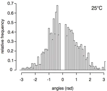
the considered species is again required in order to evaluate the feasibility of such dedicated experiments and to make sure that the behaviors in the intended experiments will be identical to those at work in the initial collective conditions. In [38], the first of these experiments consisted in introducing a single ant in the empty arena, following it during its thigmotactic behavior along the arena border and measuring the successive time intervals spent in the clockwise or counterclockwise direction. This allowed to check that the corresponding survival curve was indeed exponential, which validated the memoryless and instanta-neous turning assumptions, and to measure the direction change frequency as the inverse of the average value of the measured time intervals. Very similar is the experiment in which a single object carrying ant was followed in the empty arena leading to the evaluation of dropping frequency. Figure 4 illustrates the kind of fitting qualities that are typical of such validation and inversion exercises in the most successful cases.

Coupled validations and parametric inversions But less favorable conditions are very commonly encountered as soon as the components of the behavioral model cannot be easily isolated. It is indeed often