Analyse statistique de la pauvreté et des inégalités

AVIS

Ce document a été numérisé par la Division de la gestion des documents et des archives de l’Université de Montréal.

L’auteur a autorisé l’Université de Montréal à reproduire et diffuser, en totalité ou en partie, par quelque moyen que ce soit et sur quelque support que ce soit, et exclusivement à des fins non lucratives d’enseignement et de recherche, des copies de ce mémoire ou de cette thèse.

L’auteur et les coauteurs le cas échéant conservent la propriété du droit d’auteur et des droits moraux qui protègent ce document. Ni la thèse ou le mémoire, ni des extraits substantiels de ce document, ne doivent être imprimés ou autrement reproduits sans l’autorisation de l’auteur.

Afin de se conformer à la Loi canadienne sur la protection des renseignements personnels, quelques formulaires secondaires, coordonnées ou signatures intégrées au texte ont pu être enlevés de ce document. Bien que cela ait pu affecter la pagination, il n’y a aucun contenu manquant.

NOTICE

This document was digitized by the Records Management & Archives Division of Université de Montréal.

The author of this thesis or dissertation has granted a nonexclusive license allowing Université de Montréal to reproduce and publish the document, in part or in whole, and in any format, solely for noncommercial educational and research purposes.

The author and co-authors if applicable retain copyright ownership and moral rights in this document. Neither the whole thesis or dissertation, nor substantial extracts from it, may be printed or otherwise reproduced without the author’s permission.

In compliance with the Canadian Privacy Act some supporting forms, contact information or signatures may have been removed from the document. While this may affect the document page count, it does not represent any loss of content from the document.

Analyse statistique de la pauvreté et des inégalités

par

Marne Astou Diouf

Département de sciences économiques Faculté des arts et des sciences

Thèse présentée à la Faculté des études supérieures en vue de l'obtention du grade de

Philosophiae Doctor (Ph.D.) en sciences économiques

Mai 2008

Faculté des études supérieures

Cette thèse intitulée:

Analyse statistique de la pauvreté et des inégalités

présentée par

Marne Astou Diouf

a été évaluée par un jury composé des personnes suivantes:

Prof. Yves Sprumont : président-rapporteur Prof. Jean-Marie Dufour: directeur de recherche

Prof. Silvia Gonçalves : membre du jury

Prof. Russell Davidson: examinateur externe (McGill University)

Malgré les larges écart-types estimés dans plusieurs études de pauvreté et d'inégalités empiriques, la plupart des études dans ce domaine n'ont pas recours à l'inférence statis-tique. Deux types d'inférence sont généralement utilisés pour les mesures de pauvreté et d'inégalités: les distributions asymptotiques et le bootstrap. Bien que ces méthodes puis-sent ne pas être toujours fiables, aucune étude n'a encore proposé de méthode d'inférence exacte valide pour de tels problèmes. Nous proposons de telles méthodes.

Dans le premier article, nous construisons des bandes de confiance pour des fonctions de distribution en inversant des tests d'adéquation basés sur des statistiques de Kolmogorov-Smirnov (KS) standardisées et améliorées. Le test de KS, bien que populaire, ne per-met pas de discriminer grandement entre les distributions qui diffèrent le plus dans les queues. Pour corriger ce problème, des statistiques de KS pondérées basées sur les principes de Wald, du multiplicateur de Lagrange et du ratio de vraisemblance ont été proposées respectivement par' Anderson et Darling (1952), Eicker (1979) et Berk et Jones (1979). Toutefois, ces dernières souffrent de problèmes dus à leurs dénominateurs qui peuvent être proches de zéro. Pour y remédier, nous proposons des statistiques de KS améliorées obtenues en ajoutant un terme de régularisation au dénominateur des sta-tistiques d'Anderson-Darling et d'Eicker. Nous en déduisons des bandes de confiance exactes pour les fonctions de distribution et montrons que, dans le cas continu, ces ban-des de confiance sont indépendantes de la distribution testée sous l'hypothèse nulle et qu'elles sont conservatrices dans le cas non continu tout en bénéficiant de propriétés de monotonicité qui améliorent les bandes de confiance sans altérer leur fiabilité.

Dans les deuxième et troisièmes articles, nous proposons des intervalles de confiance exacts pour les mesures de pauvreté de Foster, Greer et Thorbecke (FGT, 1984) et les mesures d'inégalités les plus populaires, respectivement. Nous observons d'abord que ces mesures peuvent se réécrire comme des fonctions de moyennes de variables aléatoir~s, ces dernières étant elles-mêmes des fonctionnelles de fonctions de distribution de variables bornées et non bornées. Ensuite, nous utilisons des techniques de projection pour déduire des intervalles de confiance à distance finie pour la moyenne d'une variable aléatoire

bornée à partir de bandes de confiance de la fonction de distribution sous-jacente. Lorsque la variable aléatoire n'est pas bornée, nous proposons un principe de projection généralisé qui s'applique aux fonctions de distributions dont les queues sont bornées par des lois de Pareto. Enfin, nous appliquons ces procédures aux mesures de pauvreté FGT et aux mesures d'inégalités (les mesures d'entropie généralisée, de déviation logarithmique et d'Atkinson et les indices de Theil, de Lorenz, de Gini et de variation logarithmique). Dans les trois articles, des études Monte Carlo sont effectuées pour analyser la per-formance des méthodes d'inférence et illustrer le choix du paramètre de régularisation. Elles montrent que les statistiques régularisées donnent des tests plus puissants que celles existantes, lorsqu'elles sont appliquées à des distributions qui diffèrent le plus dans les queues. De même, les bandes de confiance de fonctions de distribution et les intervalles de confiance pour la moyenne basés sur ces statistiques produisent de meilleurs résultats. Dans certains cas, les intervalles asymptotique et bootstrap ne produisent pas de résultats fiables alors que les intervalles proposées sont robustes et plus courts. Pour illustration, nous analysons dans les articles 2 et 3 les profils de pauvreté et 'd'inégalités des ménages ruraux au Mexique en 1998 en utilisant des données du programme PROGRESA. Les résultats montrent que les intervalles asymptotiques sont souvent trop petits pour être réalistes alors que l'intervalle bootstrap r>eut exploser. L'analyse montre que le profil de pauvreté des ménages Mexicains dépend grandement du type de chef de ménage: les niveaux de pauvreté et d'inégalités des ménages dont le chef est un homme ou est éduqué sont moins élevés que ceux des autres ménages. De ce fait, les mesures destinées à ré-duire le taux d'illettrisme et à sécuriser le revenu des ménages dont le chef est une femme pourraient aider à réduire la pauvreté et les inégalités dans le Mexique rural.

Mots clés: inférence exacte; Kolmogorov-Smirnov ; Anderson-Darling; Eicker ; pauvreté ; inégalité ; moyenne ; régularisation; distribution de Pareto.

Summary

Despite the growing interest in poverty and inequality studies and the large standard errors found in many empirical studies, most of the work in this area neglects statistical inference. Two types of inference procedures for poverty and inequality measures have been considered: asymptotic distributions and bootstrapping. These methods can be . quite unreliable, even with fairly large samples, but no study has proposed provably

valid exact inference procedures for such problems. We propose such ones.

In the first paper, we build nonparametric confidence bands for distribution functions by inverting goodness-of-fit tests based on improved standardized Kolmogorov-Smirnov sta-tistics (KS, henceforth). Despite its popularity, the KS test do es not allow to discriminate a lot between distributions that differ mostly through their tails. To correct this draw-, back, weighted KS statistics based on the three common principles in econometrics (the Wald, Lagrange multiplier, and likelihood-ratioprinciples) are proposed respectively by Anderson and Darling (1952), Eicker (1979), and Berk and Jones (1979). However, they also suffer from drawbacks because standard errors can be very close to zero. To correct these, we propose improved weighted KS statistics obtained by adding a regularization term in the denominator of the Anderson-Darling and the Eicker statistics and derive from them exact nonparametric confidence bands for distribution functions. We show that in the continuous case, these confidence bands are independent of the distribution assumed under the null hypothesis and are conservative for noncontinuous distributions. In the noncontinuous case, we derive monotonicity properties to narrow the confidence bands without altering their reliability.

In the second and third papers, we develop such inference methods for the Foster, Greer and Thorbecke (FGT, 1984) poverty measures (paper 2) and the most popular inequal-ity measures (paper 3): the generalized entropy measures, the Theil index, the Lorenz curve, the Gini index, the Atkinson measures, the mean logarithmic deviation, and the logarithmic variation. We first observe that these poverty and inequality indicators can be interpreted as functions of the expectations of random variables which are themselves functional of distribution functions, where the involved variables can be either bounded

or unbounded. Using projection techniques, we then derive finite-sample nonparametric confidence intervals for the mean of a bounded random variable from confidence bands for the distribution of the underlying variable. When the random variable is unbounded, we propose a generalized projection principle for distribution functions which tails are bounded by a Pareto distribution. Then, we apply these procedures to the FGT poverty measures and to inequality measures.

Monte Carlo simulations are performed in the three papers to study the relative perfor-mance of the inference methods and illustrate how to choose the regularization parame-ter. The results show that the regularized statistics yield more powerful goodness-of-fit tests than the existing ones when applied to distributions with more discrepancy in the tails. Likewise, the CBs for distribution functions and the confidence intervals based on these regularized statistics have a better performance. The simulations show that asymptotic and bootstrap confidence intervals for the mean can fail to provide reliable inference, while the proposed methods are robust and yield shorter confidence intervals. As an illustration, we analyze the profile of poverty and inequality of Mexico in 1998 using households' survey data (papers 2 and 3). The results show that the widths of the asymptotic confidence intervals are often too small to be realistic while those of the bootstrap can be 10 times larger than the widths delivered by exact methods. The study shows that the poverty profile of Mexican households depends greatly on the type of households' head: poverty levels and inequality among households with a male head or an educated head are much smaller than those among other households. Hence, policies aimed at reducing illiteracy and at securing the income of households with a female head could help reduce poverty and inequality in rural Mexico.

Keywords : nonparametric inference; Kolmogorov-Smirnov; Andérson-Darling; Eicker; empirical distribution; mean; poverty; in~quality; regularization; Paretian heavy tail. JEL codes: COI, C12, C14,

011.

Table des matières

Sommaire

Summary Liste des tables Liste des graphiques Dédicace, , , '.' Remerciements Introduction générale , 1 III ix xi xii xiii 1

1 Improved exact nonparametric confidence bands and tests for distrib-ution functions based on standardized empirical distribdistrib-ution functions 7 1.1 I n t r o d u c t i o n , . . . , . . . 9 1.2 Distributional properties of goodness-of-fit statistics based on empirical

distribution functions . . . . : . . . 11

1.2,1 Pivotality and conservativeness 12

1.2.2 Special case: the Kolmogorov-Smirnov statistic and confidence band 18 1.3 Implementation as a Monte -Carlo test . . . 20 1.4 Application to the Anderson-Darling, Eicker, and Berk-Jones type

statis-tics and confidence bands. . . , . . . _ . _ . . . . . 22 1.4.1 The Anderson-Darling and Eicker statistics and confidence bands 23 1.4.2 The Berk-Jones type statistic and confidence band . . . 26 1.5 Regularized Anderson-Darling and Eicker-type statistics and confidence

bands . . . , . . . 30

1.5.1 Regularization . . . . 1.5.2 Selection of the regularization parameter (n 1.6 Monte Carlostudy . . . " .

30 33 35 1.6.1 Êffect of the regularization parameter ( . 35 1.6.2 Relative performance of the EDF-based goodness-of-fit tests 38 1.6.3 Performance of confidence bands for distribution functions

1.7 Conel usion. . . . 1.8 Appendix 1: Proofs of propositions and corollaries 1.9 Appendix 2: Details of computation . . . .

2 Improved nonparametric inference for the mean of a bounded random variable with application to poverty measures

2.1 2.2

Introduction . . . .

Confidence intervals for the mean of a bounded random variable 2.2.1 Asymptotic methods

2.2.2 Exact methods . . .

2.3 Projection methods for building confidence intervals for the mean of a 43

47

50 53 64 66 69 69 71

bounded random variable. . . .. 73 2.4 Nonparametric confidence intervals for the mean of a bounded random

variable . . . . 79 2.4.1 Three principles for building confidence intervals . 79 2.4.2 Confidence intervals based on the Kolmogorov-Smirnov statistic 81 2.4.3 Confidence intervals based on weighted Kolmogorov-Smirnov

sta-tistics . . . 83 2.4.4 Confidence interval based on likelihood ratio-type statistics . 93 2.5 Properties of confidence intervals in the continuous and noncontinuous cases 96 2.6 Choosing the values of parameter ( . . . . 99 2.7 Application to the Foster, Greer, and Thorbecke poverty measures 101

2.8 Monte Carlo study 103

2.8.2 Results . . . . 2.9 Empirical illustration

106 109 2.9.1 Analysis of the poverty profile of rural households in Mexico 111 2.9.2 Analysis of the profile of poverty of the Mexican households

tar-geted by PROGRESA 117

2.10 Conclusion. . . 123

2.11 Appendix 1: Simulated critical points of the statistics 130 2.12 Appendix 2: Proofs of theorems and propositions . . . 134 3 Finite-sample nonparametric inference for inequality measures 158

3.1 Introduction . . . . 3.2 Desirable properties for inequality measures

160 162 3.3 The inequality measures . . . 165 3.4 Asymptotic confidence intervals for the generalized entropy class of index 167

3.4.1 Confidence intervals when fJ =1= 0,1 . . . 3.4.2 Confidence interval for the Theil index

3.5 Nonparametric confidence intervals for generalized entropy class of index 167 168

when income is bounded . . . 169 3.5.1 Nonparametric confidence intervals when fJ =1= 0,1 170 3.5.2 Nonparametric confidence intervals when fJ = 1 . 175 3.6 Finite-sample confidence intervals for the mean of a random variable. 178 3.6.1 Confidence intervals for the mean of a lower bounded random variable 179 3.6.2 Confidence interval for the mean of an unbounded random variable 191 ,3.7 Application to inequality measures when income is positive. . . .. 197

3.7.1 Confidence i~tervals for the class of generalized entropy index when

fJ 0,1 . . . 199 3.7.2 Confidence intervals for the Theil index. 200 3.7.3 Confidence interyals for the mean logarithmic deviation, the

loga-rithmic deviation, and the Atkinson inequality measures 3.7.4 Confidence intervals for the Lorenz curve .

205 207

3.7.5 Confidence intervals for the Gini index 3.8 Monte Carlo study . .

3.9 Empirical illustration 3.10 Conclusion. . . .

3.11 Appendix: Proof of theorems and propositions Conclusion générale 209 210

214

218

222 234

Liste

des tableaux

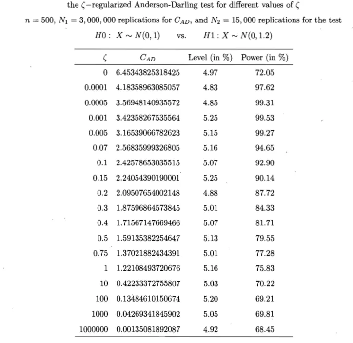
Table 1.1. Effect of the regularization parameter: Critical values, level, and 36 power of the (-regularized Anderson-Darling test for different values of (

Table 1.2 .. Effect of the regularization parameter: critical values, level, and 38 power of the (-regularized Eicker test for different values of (

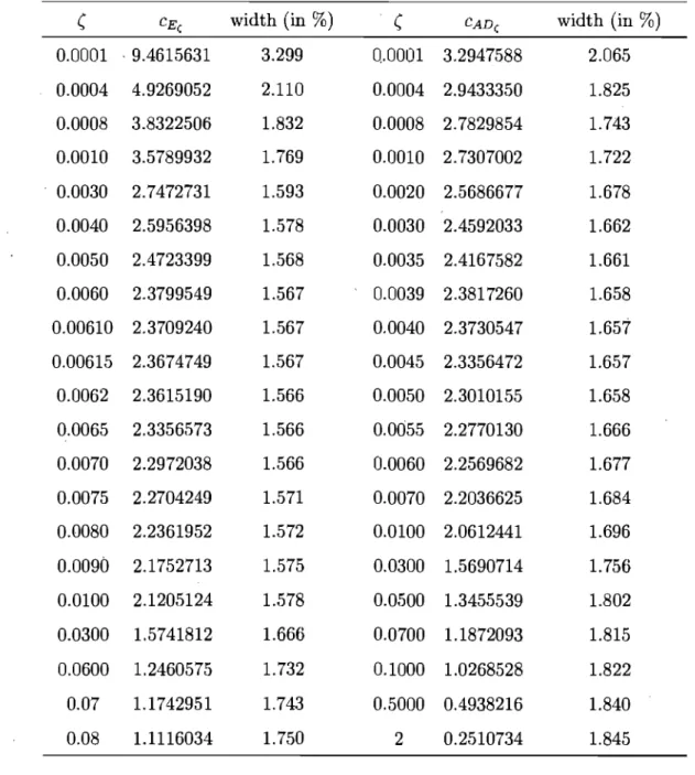
Table 1.3. Level and power of the EDF-based tests 39 Table 1.4. Simulated critical points of empirical distribution-based statistics 46 and width of the corresponding confidence bands in the tails of distributions Table 2.1 : Choice of ( : simulated level and power of the Kolmogorov- 105 Smirnov based tests for different values of (

Table 2.2: Simulated confidence intervals for the FGT poverty measure 108 P2(Y, z)

Table 2.3: Choice of (E and (AD based on an auxiliary sample of nI

=

1000

Table 2.4: Mexican households: Confidence intervals for the FGT poverty measure P2 (Y, z) for different types of households' h.eads

Table 2.5: Choice of (E and (AD based on an auxiliary sample of nI

=

100

Table 2.6: Mexican householdsin PROGRESA: Confidence intervals for P2 (Y, z) for different types of households' heads

Table 2.7: Choice of (E and (AD based on an auxiliary sample of nI

=

200 112 114 118 119 124

Table 2.8: Mexican households in PROGRESA: Confidence intervals 125 for P2

(Y,

z) for different types of households' heads .

Table 3.1: Simulated confidence intervals for the Theil index

11

213 Table 3.2: Mexican households in PROGRESA: Confidence intervals 217 for l_cini for different types of households' heads

Table 3.3: Mexican households in PROGRESA: Confidence intervals 219 for l_cini for different types of households' heads

Liste des graphiques

Graph 1.1. Level and power of the EDF-based tests Ho: X rv N(O, 1) vs. 40

Hl : X rv N(O, 0") for 0"

=

0.5, 0.55, 0.6, ... , 1.5

Graph 1.2. Level and power of the EDF-based tests Ho: X rv N(O, 1) vs. 42

Hl : X rv N(O.l, 0") for 0"

=

0.5, 0.55, 0.6, ... , 1.5

Graph 1.3. Empirical distribution function-based confidence bands for 44 the distribution function N(O, 1)

A ma mère: Yaye Awa N'Diongue. Sans toi, rien de tout cela n'aurait été possible. A mes soeurs chéries: Diago, Fatoumata Binetou, Awa et la toute choyée Oum y Khairy. Vous me manquez tellement.

Itenaercienaents

Je remercie du fond du coeur mon directeur de thèse Jean-Marie Dufour pour son encadrement, sa patience et son soutien à la fois moral et financier tout au cours de ces longues années.

Je remercie le personnel administratif du département de sciences économiques de l'Université de Montréal et du CIREQ pour toute l'aide apportée durant la préparation de ce doctorat. Je remercie le département de sciences économiques de l'Université de Montréal, le CIREQ, la Chaire de Recherche du Canada en économètrie (Jean-Marie Dufour) et la Chaire William Dow en économie politique (Université McGill) pour le soutien financier alloué.

Je remercie chaleureusement Nour Meddahi pour m'avoir aguillé durant les premières. années si importantes de ce processus. Je remercie également tout le corps professoral du doctorat de sciences économiques de l'Université de Montréal pour la formation apportée et leur aide à divers moments.

Merci également à toutes les personnes qui ont de près ou de loin aidé à la réalisation de ce projet si cher. Merci à Peter Lanjouw pour m'avoir fourni gracieusement les données utilisés pour l'application empirique (voir page 110). Merci à Albert Touna Marna pour son aide très apprécié. Merci à un collègue du Fonds Monétaire International qui se reconnaitra, pour ses encouragements aux premières aurores de chaque journée. Un grand merci à une personne spéciale, une soeur de coeur: Kadiata Kane, pour avoir été là aux moments cruciaux.

J'envoie mes sincères remerciements à mes amis et aux membres de ma famille, petite et grande, pour leur soutien, leur aide et pour avoir cru en moi.

Introduction Générale

Durant les dernières décennies, il y eut un intérêt croissant pour les études de pauvreté et d'inégalités. Toutefois, en dépit des larges écart-types trouvés dans les études em-piriques, la plupart des analyses dans ce domaine sont restées descriptives, ne procédant

p~ à une inférence statistique rigoureuse. Deux types de procédures inférentielles ont été proposés: les distributions asymptotiques et le bootstrapj voir Beran (1988), Kakwani (1993), Rongve (1997), Mills et Zandvakili (1997), Dardanoni et Forcina (1999), Biewen (2002), Davidson et Duclos (2000), Zheng (2001) et Davidson et Flachaire (2007). La plupart de ces études recommandent l'utilisation du bootstrap au lieu des approxima-tions asymptotiques parce que ce dernier peut ne pas être fiable quand il est appliqué

à des échantillons de taille petite voire modérée. Ces études reconnaissent cependant également les limites du bootstrap standard, en particulier que la procédure peine sou-vent à performer en présence de distributions avec des queues épaisses qu des masses de probabilité comme c'est le cas dans les études de pauvreté et d'inégalités. Dans ce cadre, des procédures spécifiques doivent être implémentées pour améliorer les résultats du bootstrap mais le choix de la procédure adéquate requiert de connaître la nature du problème à l'origine de l'échec du bootstrap standard, ce qui n'est pas trivial quand la distribution étudiée est inconnue. Des études montrent que les méthodes d'inférence as-ymptotique et bootstrap ne produisent pas de résultats satisfaisants lorsque appliquées aux mesures d'inégalités. Entre autres, Davidson et Flachaire (2007) montrent que les distributions asymptotiques donnent une pauvre approximation des véritables distribu-tions des statistiques quand la taille de l'échantillon est petite ou moyenne. Ils montrent de plus que le bootstrap Li.d. donne des tests de pauvre niveau lorsque appliqué à l'indice d'inégalité de Theil avec une distribution de revenue Singh-Maddala. En dépit de toutes ces problèmes, aucune étude n'a, à notre connaissance, proposé de méthode d'inférence non paramétrique à distance finie valide pour les mesures de pauvreté et d'inégalités. Dans cette thèse, nous nous intéressons à ce problème.

fonctions de distribution. La première est basée sur le test de KS (KS, ci-dessous) qui est l'un des tests non paramétriques d'adéquation de lois le plus populaire. Ce dernier est fondé sur la statistique de KS qui est le supremum sur toutes les observations de la différence entre la fonction de distribution supposée sous l'hypothèse nulle et la fonction de distribution empirique de l'échantillon. Le test rejette la fonction de distribution testée si elle est trop loin de celle empirique, le seuil de rejet étant défini par le point critique de la statistique. Le test doit sa popularité ~ l'une de ses propriétés très pratiques: la distribution de la statistique de KS est indépendante de la fonction de distribution supposée sous l'hypothèse nulle lorsque celle-ci est continue et par conséquent, les points critiques de la statistique ne dépendent pas de la distribution testée et le même ensemble de points critiques peut être utilisé pour tester toutes les distributions continues. En inversant ce test, il est possible de construire une bande de confiance pour les fonctions de distribution qui bénéficient des mêmes propriétés que le test de KS.

Malgré le fait que le test de KS est pratique, il souffre d'un inconvénient majeur: il

discrimine faiblement entre les distributions qui diffèrent principalement au niveau de leurs queues, ce qui altère les performances du test et des bandes de confiance. En particulier, la bande de confiance de KS a souvent été critiquée en raison de son caractère uniforme. Sa largeur est constante pour toutes les observations; par conséquent, ses bornes ne convergent pas vers 0 et 1 dans les queues de distributions, contrairement aux fonctions de distribution qu'elles bornent. Pour corriger cette contreperformance, nous utilisons des statistiques pondérées de KS basées sur les trois principes fondamentaux en économétrie:. les principes de Wald, du multiplicateur de Lagrange et du ratio de vraisemblance. Ces statistiques ont été proposées par Anderson et Darling (1952), Eicker (1979) et Berk et Jones (1979), respectivement.

Les statistiques d'Anderson-Darling et d'Eicker sont des statistiques de KS standardisées pour lesquelles la différence entre la distribution théorique et celle empirique est divisée par une sorte d'écart-type. ,Ces statistiques permettent une meilleure discrimination entre les distributions qui diffèrent principalement au niveau de leurs extrémités. En utilisant ces statistiques, nous proposons des bandes de confiance exactes dont la largeur diminue

au fur et à mesure que les observations s'éloignent du centre de la distribution. Toutefois, les statistiques d'Anderson-Darling et d'Eicker ont leurs propres inconvénients. Les poids au niveau des dénominateurs de ces statistiques deviennent très proches de zéro pour les observations dans les queues, ce qui induit un comportement erratique des statistiques. Pour y remédier, nous proposons des statistiques obtenues par l'ajout d'un terme de régularisation au dénominateur "des, statistiques d'Anderson-Darling et d'Eicker. Ces statistiques conservent les avantages des statistiques de KS pondérées, mais ne souffrent pas d'instabilité. En inversant les statistiques régularisées, nous proposons des bandes de confiance exactes améliorées pour les fonctions de distribution.

La statistique de Berk-Jones est le supremum, sur toutes les observations, du ratio de log-vraisemblance entre les fonctions de distribution empirique et théorique utilisée comme distance entre ces deux fonctions. Il a été prouvé que cette statistique domine toutes les statistiques pondérées de KS, au sens de Bahadur et constitue donc une bonne référence de comparaison pour nos méthodes d'inférence. Cette statistique a été utilisée par Owen (1995) pour construire une bande de confiance non paramétrique pour les fonctions de distribution continues.

Nous montrons que dans le cas continu, les distributions des statistiques basées sur des fonctions de distribution empiriques sont indépendantes de la fonction de distribution testée sous l'hypothèse nulle, ainsi que leurs points critiques. Par conséquent, les ban-des de confiance qu'elles permettent de construire dépendent de la distribution testée uniquement par l'échantillon. Ces bandes sont construites avec le même ensemble de points critiques pour toutes les fonctions de distribution continues, ce qui les rend facile à calculer. Pour les fonctions de distribution discontinues, nous dérivons des propriétés de monotonicité qui exploitent l'emboîtement des ensembles images de différentes distri-butions pour réduire la largeur des intervalles de confiance sans toutefois en altérer la fiabilité.

Dans les deuxième' et troisième articles de cette thèse, nous proposons des inter-valles de confiance pour la moyenne d'une variable aléatoire que nous appliquons aux mesures de pauvreté de Foster, Greer et Thorbecke (1984, ci-dessous FGT) et aux mesures

d'inégalités les plus populaires: la mesure d'entropie généralisée--qui inclut l'indice de Theil, la courbe de Lorenz, l'indice de Gini, la mesure d'Atkinson, la mesure de déviation logarithmique et l'indice de variation logarithmique. Pour ce faire, nous observons que les mesures de pauvreté peuvent se réécrire comme la moyenne d'une variable aléatoire bornée--un mélange entre une variable aléatoire continue et une masse de probabilité au seuil de pauvreté--et proposons que les méthodes d'inférence nonparamétrique exactes pour la moyenne d'une variable aléatoire bornée leur soient appliquées (article 2).

A

première vue, ce problème paraît ne pas avoir de solution. En effet, d'après Bahadur et Savage (1956), il est impossible d'établir une inférence nonparamétrique pour la moyenne d'une variable aléatoire sur la base d'observations indépendantes et identiquement dis-tribuées provenant d'une distribution inconnue dont la moyenne est finie (voir Dufour (2003) pour de plus amples détails). Toutefois dans notre cas, la nature bornée de la variable aléatoire étudiée donne une restriction suffisante pour permettre d'effectuer une inférence nonparamétrique. De tels intervalles de confiance pour la moyenne d'une vari-able aléatoire bornée sont.proposés par Anderson (1969), Hora et Hora (1990) et Fishman (1991). Sutton et Young (1997) comparent les performances de ces méthodes à celles des méthodes bootstrap et asymptotique à l'aide de lois Beta. Ils montrent que les intervallès asymptotique et bootstrap ont une mauvaise probabilité de couverture en échantillon fini alors que les méthodes exactes sont très fiables mais produisent des intervalles plus larges que les premiers.

Nous observons que les mesures FGT sont des moyennes de variables aléatoires bornées qui sont elles-mêmes des fonctionnelles de fonctions de distribution et utilisons des tech-niques de projection pour déduire des intervalles de confiance à distance finie pour la moyenne d'une variable aléatoire bornée à partir de bandes de confiance de la fonction de distribution sous-jacente. Enfin, nous appliquons ces intervalles de confiance aux mesures de pauvreté FGT.

De façon similaire, nous montrons que la plupart des mesures d'inégalités peuvent se réécrire comme une fonction de moyennes de deux variables aléatoires dont l'une ou les deux peuvent ne pas être bornées (article 3). Dans ce cas, nous proposons une

généralisation du principe de projection utilisé pour les variables bornées aux vari~bles

non bornées, sous l'hypothèse que les queues de distribution étudiées sont bornées par des distributions de Pareto (voir Davidson et Flachaire, 2007 pour l'utilisation d'hypothèses similaires dans des procédures bootstrap). D'abord, nous observons que la moyenne d'une variable peut s'interpréter comme la moyenne pondérée d'une variable bornée et d'une variable non bornée, cette dernière étant la moyenne de la queue de distribution. En utilisant les techniques de projection utilisées dans le deuxième article, nous développons des intervalles de confiance pour la moyenne de la partie bornée de la variable aléatoire. Ensuite, nous établissons des bornes inférieure et supérieure pour la partie non bornée de la variable en utilisant l'hypothèse que les queues de distribution de ladite variable sont bornées par des lois de Pareto et appliquons les inégalités de Bonferroni pour calculer le niveau de l'intervalle de confiance ainsi construit. Enfin, nous appliquons ces méthodes d'inférence pour calculer des intervalles de confiance pour les mesures d'inégalités à partir de bandes de confiances des distributions sous-jacentes.

Tous ces intervalles de confiance bénéficient des mêmes propriétés pratiques que les bandes de confiance dont ils sont issus: pivotalité, conservation, monotonicité, etc.

Dans les trois articles, des études Monte Carlo sont effectuées pour analyser la per-formance des méthodes d'inférence et illustrer le choix du paramètre de régularisation. Elles montrent que les statistiques régularisées donnent des tests plus puissants que celles existantes, lorsqu'elles sont appliquées à des distributions qui diffèrent le plus dans les queues. De même, les bandes de confiance de fonctions de distribution et les intervalles de confiance pour la moyenne basés sur ces statistiques 'produisent de meilleurs résul- . tats. Dans certains cas, les intervalles asymptotique et bootstrap ne produisent pas de résultats fiables alors qu'en revanche les intervalles exacts sont robustes à la distribution sous-jacente et à la taille de l'échantillon. Les intervalles de confiance proposés offrent une probabilité de couverture généralement plus grande que le niveau nominal tout en restant informatifs. Pour illustration, nous analysons dans les articles 2 et 3 les profils de pauvreté et d'inégalités des ménages ruraux au Mexique en 1998 en utilisant des données

du programme PROGRESA.l Les résultats montrent que les intervalles asymptotiques sont souvent trop petits pour être réalistes alors que l'intervalle bootstrap peuvent ex-ploser, donnant des intervalles de largeur 10 fois supérieure à celles des méthodes exactes. L'étude montre qu'en moyenne, les ménages ruraux ciblés par PROGRESA n'ont pas un niveau de pauvreté très élevé. Toutefois, le profil de la pauvreté dépend grandement du sexe du chef de famille. Le niveau de pauvreté et d'inégalités des ménages avec à leur tête un individu male est beaucoup plus faible que celui des ménages ayant une femme à leur tête. En outre, les ménages avec un chef éduqué à leur tête semblent être plus susceptibles d'échapper à la pauvreté et aux inégalités que les ménages avec un chef non-instruit. Ces conclusions apportent des suggestions dans l'élaboration des politiques visant à réduire la pauvreté et les inégalités dans les régions rurales du Mexique. Les politiques visant à

réduire l'analphabétisme des membres des ménages dans ces communautés peuvent être efficaces dans la réduction de la pauvreté. Les programmes d'éducation devraient viser les enfants et les adultes, en particulier les chefs de ménages afin de produire un effet im-médiat. De même, les politiques visant à assurer le revenu des ménages ayant une femme à leur tête pourrait aider à réduire la pauvreté et les inégalités dans les régions rurales du Mexique. Un exemple de telles politiques peuvent être des réformes visant à garantir la propriété foncière pour les femmes ou à l'amélioration de la productivité du travail pour les ménages avec une femme à leur tête, cette dernière étant moins productive dans des activités demandant un effort physique intensif telles que l'agriculture.

Improved exact nonparametric

confidence bands and tests for

distribution functions based on

standardized empirical distribution

. functions

Abstract

Goodness-of-fit tests àre of great interest in econometrics. In many procedures, especially in parametric ones, determining the distribution from which the sample cornes from may be an important step. The Kolmogorov-Smirnov (KS, henceforth) test is one of the most popular nonparametric goodness-of-fit tests. However, it does not allow to discriminating a lot between distributions that differ mostly through their tails. Weighted KS statistics have been proposed by Anderson and Darling (1952) and Eicker (1979) to improve the performance of the test in the tails but they suffer from important drawbacks.

We propose improved weighted KS statistics to correct these limits. These statistics are obtained by adding a regularization term in the denominator of the Anderson-Darling and the Eicker statistics. They retain the advantages of the weighted KS statistics but their denominators do not become close to 0 in the tails of distributions as it is the case for the original statistics. We derive exact nonparametric confidence bands (CBs, henceforth) for distribution functions using the weighted and regularized KS statistics. We show that in the continuous case, these CBs are independent of the distribution assumed under the null hypothesis and are conservative for noncontinuous distributions. In the noncontinuous case, we derive monotonicity properties that exploit embeddedness of the image sets of different distributions to narrow the CBs without altering their reliability.

Monte Carlo simulations are performed to study the relative performance of the inference methods and illustrate how to choose the regularization parameter. The results S;tlOw that the regularized statistics yield more powerful goodness-of-fit tests than the existing ones when applied to distributions with more discrepancy in the tails. Likewise, the CBs for distribution functions based on these regularized statistics are of better performance.

1.1 Introduction

The problem of determining the distribution from which a sample comes from is of great interest in statistics and econometrics. Instead of using an asymptotic law, it is often desirable and even crucial to ~ow the actual distribution of a sam pIe before applying further econometric procedures, in particular parametric ones. Several goodness-of-fit tests have been proposed. They test the null hypothesis that a sample follows a given distribution-which generally needs to be fully specified-against the alternative that the sample does not follow this distribution. Parametric tests have been proposed by Shapiro and Wilk (1965), Lilliefors (1967), Chambers (1983)-probability plots, etc. Likewise, non-parametric procedures have been provided by Snedecor and Cochran (1989)-Khi square test, Anderson and Darling (1952), Kolmogorov (1941), Smirnov (1944), Cramer (1928), Von Mises (1931), etc.

The Kolmogorov-Sniirnov (KS, henceforth) test is one of the most popular nonpara-metric goodness-of-fit tests. It is based on the KS statistic which is the supremum over all observations of the difference between the distribution function assumed under the null hypothesis and the empirical distribution function of the sample. The test rejects the distribution function assumed under the null hypothesis if it is too far from the empirical distribution function, the threshold being defined by the critical point of the KS statistic. The test owes its popularity to a convenient property: the distribution of the KS statistic is independent of the distribution function being tested under the null hypotheses when the latter is continuous. Hence, the critical points of the statistic are· not contingent bn the assumed distribution and can be used to test any continuous distribution function. These critical points have been tabulated by several authors and are widely published. Inverting the test allows one to build confidence bands (CBs, henceforth) for distribution functions which also benefit from the pivotality of the KS statistic.

Even though the KS statistic is convenient, it has low power to discriminate a lot between distributions that differ mainly through their tails. This property alters the performance of the KS test and CB. In particular, the KS confidence band has often been criticized because of its uniform nature: its width is constant for all observations

and thus, its bounds do not converge to 0 and 1 in the lower and· the upper tails of the distribution, as do the distribution functions they bracket. To correct this drawback, we use weighted KS statistics based on the three common principles in econometrics: the Wald, Lagrange multiplier, and likelihood-ratio principles. These statistics have been proposed by Anderson and Darling (1952), Eicker (1979), and Berk and Jones (1979). The Anderson-Darling and the Eicker statistics are standardized versions of the KS statistic where the difference between the theoretical and the empirical distributions is divided by a kind of standard deviation. These statistics allow one to discriminate between distributions that differ mostly through their tails. Using them, we propose finite-sample nonparametric CBs whose widths decrease with observations further from the center of the distribution.

The Anderson-Darling and the Eicker statistics have their own drawbacks. The power of the goodness-of-fit test they yield is smaller than the power of the standard KS test when testing distributions with low dispersion that differ more in the center of the dis-tribution than in the tails. Moreover, the weights in the denominators of those statistics become very close to zero for observations in the tails, leading to erratic behavior of the statistics. We propose improved weighted KS statistics to correct these. These statistics are obtained by adding a regularization term in the denominator of the Anderson-Darling and the Eicker statistics. They retain the advantages of the weighted KS statistics but do not suffer from instability, improving the performance of the in.ference. By inversion of the regularized statistics, we build improved exact CBs for distribution functions.

The Berk-Jones statistics uses the supremum, over aIl observations, ofthe log-likelihood ratio of the empirical distribution function and the theoretical distribution function as a distance between these two functions. This statistic has been proved to dominate any weighted KS statistic, in the sense of Bahadur and is thus a challenging referral for our inference methods. It has been used by Owen (1995) to propose a CB for distribution functions.

In the continuous case, we show that the distributions of the empirical distribution-based statistics are pivotaI and that their critical points do not depend on the

distri-but ion function being tested under the nuIl hypothesis. Hence, the corresponding CBs depend on the distribution only through the sample; they are built using the same critical points for aIl continuous distribution functions, which make them easy to compute. For noncontinuous distribution functions, we derive monotonicity properties which exploit embeddedness of the image sets of different distributions to narrow the CBs without altering their reliability.

We compare the relative performance of the nonparametric and parametric inference methods. Monte Carlo simulations are performed to study the. power of the goodness-of-fit tests under various hypotheses. In both studies, we study carefuIly the choice of the regularization parameter. The results show that regularized statistics yield more powerful goodness-of-fit tests than the existing ones when applied to distributions with more discrepancy in the tails.

The paper is organized as foIlows. Section 2 presents the Kolmogorov-Smirnov, the Anderson-Darling and the Eicker statistics and derives the expressions to compute them.

It also shows how to invert these tests and build the CBs for distribution functions they yield. In section 3, we introduce the regularized statistics and derive explicit expressions· to compute them and to build CBs for distribution functions. Sections 4 presents the Owen CB and Section 5 derives sorne convenient properties of these CBs for continuous cases and monotonicity properties for noncontinuous distribution functions. Section 6 presents Monte Carlo results and Section 7 concludes.

1.2 Distributional properties of goodness-of-fit

sta-tistics based on empirical distribution functions

Let's define sorne notation for the remainder of the paper. Denote F, the set of aIl distribution f~nctions, F, the set of continuous distribution functions, F[a,b] the set of distribution functions with support

[a, b] ,

and IR

=

IR U, {

-oo}

U

{+oo}.

Let X be a random variable with distribution function

F(x)

E F. Denote X(l)

:S

X(2)

:S ... :S

X(n) .

empirical distribution function defined as follows: V k = 0, ... , n

(1.1)

where (X(O),X(n+l») is the support of

F(x),

which may be the realline

(-00,+00)

and X(O) ::; X(l)

:S

X(2) ::; ... ::; X(n) ::; X(n+l)'

Let's consider the following null hypothesis:

Ho(F) :

X l , " "

X n

are i.i.d. with distribution function

P[Xi ::;

x]

F(x).

(1.2)

A general statistic to test

Ho(F)

against its negation

HI(F)

is:

D

(F~,

F)

=

sup Dl

[Fn(x), F(x)].

(1.3)

-oc<x<+oc

where Dl

[Fn(x), F(x)]

is a functional of

Fn(x)

and

F(x),

which measures the distance between these two functions. In this section, we study interesting properties for statistics of the form

_{D (Fn, F)}

when

F(x)

is continuous and when it is not.

1.2.1 Pivotality and conservativeness

PROPOSI!ION 2.1. [Distribution of statistics based on empirical distribution functions when

F(x)

is continuous] Let XI, ... ,

X

n be n random variables. Let

D

(Fm F)

be a statistie of the form:

D (Fn, F)

= sup

DdFn(x) , F(x)].

-oo<x<+oo.

If F (x) is a continuous monotonie funetion, then the following identity holds almost surely:

D (Fn, F)

=

sup Dl

[H(U}, ... , Un,

U), U]

where Ui = F(Xi ), i = 1, ... ,n and

If, furthermore, Xl, . .. ,Xn are n i.i.d. observations on X with continuous distribution

function F (x) E

F,

then

D

_{(Fn, F)}

~ sup Dl

[H(U

I , ... ,

Un,

u), u] o:s:uS)

where Ui

=

F(Xi ), i

=

1, ... , n are i.i.d. with uniform U[O,I] distribution.

Proposition 2.1. states that when

F(x)

is continuous, the distribution of

D (Fn , F)

is independent of

F(x).

D

(F

n ,

F)

can be rewritten using only uniform statistics. All

statistics withgeneral form

D (Fn , F)

are pivotaI for continuous distribution functions. Re'nce, the critical points associated to those statistics are also independent of

F(x).

This property simplifies a lot the implementation of the tests and CBs associated to such statistics. A unique set of critical points is needed to compute these for all continuous distribution functions.

When

F(x)

is not continuous, the distribution of D

(F

n ,

F)

is different for each

F(x)

being tested. The associated critical points are also modified by the distribution of the sample. Renee, a new set of critical values need to be computed to implement the tests for each distribution, making the inference methods more difficult to implement. Moreover, in this case, building CBs for

F(x)

loses all interest because these are usually built to bracket unknown distribution functions using a sample of observations that cornes from the distribution under interest. To simplify the implementation of the inferen~e methods and restore the interest of CBs in the case of noncontinuous distribution functions, we propose to exploit the following properties ..

PROPOSITION 2.2. [Conservative nature of continuous case critical points] Let Xl,' .. ,Xn be n i.i.d. observations on X and Fn(x) the corresponding empirical distrib-ution junction. Let F (x) E

F

be a continuous distribution function and G (x) E F a

non-continuous one. For any level a, 0 ::; a ::; 1, the critical value associated with D (Fn , F)

for testing the null hypothesis

Ho(F)

as defined by equation (1.2) is larger than or equal to the critical value associated with D (Fn , G) for testing the null hypothesis

Ho(G):

or equivalently

PROPOSITION 2.3. [Conservative property of continuous case CBs for distribu-tion funcdistribu-tions] Let Xl,' .. ,X

_n

be n i.i.d. observations on X and

Fn(x)

the correspond-ing empirical distribution function. Let

F(x)

E

F

be a continuo us distribution function and G(x) E F be a noncontinuous one. For any level a, 0 ::; a ::; 1, the confidence band obtained by inverling the test of the null hypothesis

Ho(F)

as defined by equation

(1.2)

using appropriate critical points with level a for D

(Fn,

F) yields a confidence band for G(x) with levellarger th an or equal to 1 -

a.

Equivalently, if

en

is defined as follows:

where

then

Propositions 2.2. and 2.3. highlight sorne interesting properties of the ernpirical distribution function-based statistics and CBs which sirnplify their irnplernentation when applied to noncontinuous distributions. Proposition 2.2. states that the critical values of

D (Fn, G)

for continuous distribution functions

F(x)

are conservative for noncontinuous functions

G(y).

Using the appropriate critical values of level a for

F(x)

provide a test

of levelless than or equal to a for G(y). Therefore, rejection of the null hypothesis with such test leads to rejection for the nominal level a. In other words, the result of the test based on

D (Fn, G)

remains Valid and one can use the conservative critical values to compute tests and CBs for noncontinuous distribution functions. Let's remember that those critical points-that applies to continuous distributions-are independent of the function being tested and are thus, identical for aIl continuous distributions. Note that these propositions hold for any continuous distribution function F(x).

Likewise, the CBs for G(y) built using appropriate critical points for continuous dis-tribution functions will be of levellarger than or equal to 1 - a. Using these properties, critical points from continuous distribution functions can be applied to any sample from a general distribution function. The resulting CBs will be of level at least equal to 1- a. Even though the conservative critical points provide valid inference for noncontinuous distribution functions, using them alters the performance of the inference. The question is how far the quality of the performed inference is affected? We assess this question using the properties of tests and CBs. Concerning the tests, when the null hypothesis is accepted with level a, the conclusion of the test remains valid for levels less than or equal to a. Conversely, when the null hypothesis is rejected with level a, it will be still rejected for levels larger than a but might be accepted for lower levels. Concerning CBs, the impact of the using conservative critical points can be studied using the level of confidence (accuracy) and the width (precision) of the CBs. Given that the CBs using conservative critical points have a higher level than the targeted one, they will be wider than the CBs with effective leve11 a. To reduce the width, exact critical values corresponding to the distribution function under interest can be computed. However, by doing this, the CBs willloose one of their major advantages. To avoid this shortcoming, we derive monotonicity properties that can be used to narrow CBs without altering their reliability. These results are based on information about the set of discontinuities of the distribution function.

PROPOSITION 2.4. [Range monotonicity of critical points] Let X}, ... , Xn be n

Let F(x) and G(y) be two distribution functions such that G(IR)

ç

F(IR). For any level a, 0 ::; a ::; 1, the critical value associated with D (Fn, F) for testing the null hypothesis Ho(F) as defined by equation (1.2) is larger than or equal to the critical value associated with _{D (Fn, G) for testing the null hypothesis Ho(G):}

PROPOSITION 2.5. [Range monotonicity of CBs for distribution functions] Let

Xl,' .. ,X_{n be n i.i.d. observations on} X and Fn(x) the corresponding empirical distrib-utionfunction. Let F(x) and G(y) be two distributionfunctions such that G(IR)

ç

F(IR). For any level a, 0 ::; a ::; 1, the confidence band obtained by inverting the test of the null hypothesis Ho(F) as defined by equation (1.2) using appropriate critical points with level a for _{D (Fn, G) yields a confidence band for G (x) with level larger th an or equal to} 1 - a. Equivalently, if en is defined as follows:

where

then

Propositions 2.4. and 2.5. generalize Propositions 2.2. and 2.3. to aIl distribution functions. It suggests that CBs can be made narrower by exploiting embeddedness of the image sets of different distributions. When studying a discontinuous distribution G (y ), .

we know that G(y) takes its values in a set VG _{which is included in [0,1]. Thus, the}

conservative CB for a continuous distribution I?rovides a CB for G(y) with level 1 - 151 greater than or equal to 1 - a. If additional information about the image set of G(y) is available-in particular, if we know there exists a distribution function with image VF

such that VG

_ç

_VF _{-then the critical points for testing F(x) can be used to derive a CB}

for

G(y)

with level 1 6₂ such that 1 a:5 1 - 6₂ :5 1 ....:.. 6_{1 ,} The CB with level 1 - 6₂ is narrower than the CB with level 1 61 while being reliable. Thus) using information ab,out the nature of the discontinuity of the random variable can be useful for providing shorter CBs for

G(y).

The more is known about the set of discontinuity points of the distribution) the better the inference will be. However, the improvement can be achieved without knowing an discontinuity points of

G(y)

and their probability masses. Hence, the main advantage of the KS confidence band, that is its independence of the assumed distribution function, is somehow preserved.

Let's consider a special case of embedded image sets. Let X be a random variable with distribution H(x) E FrO,l] snch that X is a mixture between a continuous variable bounded on (0,1] and a probability mass of H(O)

==

pat O. H(x) is continuous on (0,1] with H(O) = p and H(l) 1.

COROLLARY 2.6.

[Range

monotonicity with a mass at the lower boùndary] Let Xr,'" ,X~ be n i.i.d. observations on X_{2 and Fn(x) the corresponding empirical}

distribution function. Let FI (x) and F2 (x) be two distribution functions continuo us on (a, b] such that Pl Fl(a):5 F2(a) = P2. For any level a, 0:5 a

:5

l, the confidence band obtained by inverting the test of the null hypothesis Ho(Fl) as defined by equation (1.2) using appropriate critical points with level a for D (Fn, FI) yields a confidence band for F2(X) with levellarger than or equal to 1 - a. Equivalently, if en is defined as follows:

where

Corollary 2.6. describes the special case where the distribution function being studied is continuous everywhere exeept at the lower bound of its support. This case is very interesting because such distribution functions are quite frequent in financial studies, and poverty and inequality analysis. Moreover, this case can be easily extended to those where the discontinuity point is at the upper bound of the support or those where both the lower and the upper bounds are discontinuity points.

1.2.2

Special case: the Kolmogorov-Smirnov statistic and

con-fidence ba,nd

Let X be a random variable with distribution function F(x) E F. Denote X(l)

:s;

X(2)

:s;

... :s;

X(n) the order statistics of a sample of n Li.d. observations on X and Fn(x) the empirical distribution function of the sample. The Kolmogorov-Smirnov (KS, heneeforth) statistic is

KS

=

sup vnIFn(x) - F(x)1 (1.4)

-oo::;x::;+oo

Developing this expression allows to reexpress the KS statistic as follows:

This explicit expression is more convenient and can be used to compute the test easily. The KS is a special case of the statistic D (Fn, F) where

Henee, all properties derived for this general form of statistics apply to the KS statistic. In part icular , when applied to continuous distribution functions, the KS statistic is pivotaI and its distribution can be characterized as follows:

Seant { ' [ i

TT]

[TT

i -

1] }

K = max max - - U(i) ,max U(i) - - - ,0

where U(l)

:S

U(2)

:S ... :S

U(n) are the order statistics of a sample of n LLd. observations

of an uniform U[O,I] distribution. The critical values used to compute the KS tests are

the same for aIl F E F and thus, do not need to be simulated for each distribution. Moreover, appropriate KS critical values for testing continuous distribution functions are conservative for noncontinuous distributions. To end, this conservative. property extends to the cases of distribution functions with embedded image ·sets.

It foIlows that the KS critical point for a level Ct and a given sample size n is the same for aIl continuous distribution functions and can be used to test the hypothesis Ho : Xi '" F against the alternative one Hl : Xi "" F for aIl F E F. Exact critical points for K seant can be computed by simulation using the foIlowing 3-steps procedure:

1. Generate a sample of n i.i.d. observations from an uniform law U[O,I]

2. Compute the Kolmogorov statistic K seant for this sample using the expression Kseant

=

max {max

[i -

U(i)] , max [U(i) -

i-l]

,o}

l::St::Sn n l::St::Sn n

3. Repeat N times steps 1 and 2-N is the number of replications-and compute the critical value of level a, the (1 - a)th fractile.

Tables of the Kolmogorov-Smirnov critical points have been computed and published, for continuous distributions. Having them simplifies the test considerably and makes this goodness-of-fit test more convenient to use than the other exact methods.

The conservative property of the KS statistic has been evoked by Kolmogorov (1941) before being proved by other authors including Noether (1963) and Conover (1972). We provide in Appendix 2, a more convenient proof of this property than those provided in the literature.

The CB for F(x) with level greater than or equal to 1- a built inverting the KS test is:

(1.5)

When

F(x)

is continuous

CKS(a)

does not depend on if For a given sample size, the same critical value is used to build CBs for aIl continuous distributions. Hence, the KS confidence band depends on

F(x)

only through the sample. This simplifies a lot its computation and makes its popularity. Moreover, owing to the monotonicity of the KS critical points when applied to distributions with embedded image sets, if

F(x)

and G(y) are two distribution functions such that G(IR) ç F(IR) then the KS confidence band using adequate critical values for

F(x)

embeds the KS confidence for G(y). Hence,using information about the image set of G(y) one can build narrower CB for the latter without having to use the adequate critical values for it.

1.3 Implementation as a Monte Carlo test

In the preceding section, we studied interesting properties for statistics of the form D (Fn, F) = sup Dl [Fn(x), F(x)] . In this section, we show another important

ad--oo<x<+oo

vantage of these statistics which make them even more attractive. We show that the test of Ho(F) as defined by equation (1.2) based on these statistics can be implemented using exact randomized test procedures such as Monte Carlo tests (see Dwass (1957), Dufour (1995), Dufour and Kiviet (1998), and Dufour and Khalaf (2001)). Given that D (Fn , F)

is pivotaI under Ho(F), the Monte Carlo test based on pivotaI statistics can be applied. Given that the distribution of D (Fn, F) is noncontinuous, the standard Monte Carlo test procedure cannot be applied. In this case, a randomized tie-breaking procedure (Dufour, 1995) can be applied to test Ho(F). This procedure is a modified Monte Carlo test ad~pted for discrete distributions. It can be implemented as foIlows.

Let Do denote the test statistic computed from data and Do the observed value of Do based on specifie realized data. Do is a random variable while Do is fixed. The critical region of the test is Do

2:

Da where a is the level of the test and G(Do)

=

P (D

2:

Do 1 Do

=

Do) is the realized p-value of the test statistic Do. Suppose we can

generate N Li.d. replications Dj, j

=

1, ... ,N of D (Fn, F) under Ho(F). The foIlowing steps apply:

• Draw N

+

1 Li.d. variates W

_o,

W1 , •.• , WN independently of Dj.

• Order the pairs (D j, Wj ) following the lexicographic criterion:

• Compute an empirical p-value function:

where 1 N N 2::)1[0,00)

(x

j=l 1 N Dj)

+

N 2::)'101 (Dj -

x)

11[0,00) (Wj - W

o) .

j=l

.

PN(X)

is the empirical probability that a value as extreme or more extreme than x is realized if

Ho(F)

is true. Note that

NON (x)

is the number of simulated statistics which are greater or equal to x.

• Compute the associated Monte Carlo critical region-which is a randomized critical region-as:

(1.6)

where

_PN(Do)

may be interpreted as an estimate of

C(Do).

Given

Do

=Do, ~v(Do)

can be interpreted as a realized Monte Carlo p-value associated with

Do.

Thus if

N is chosen such that

a

(N

+

1) is an integer, the critical region (1.6) has the same size as the critical region

C(Do) ::; a.

Moreover,

p

r;:;

(D )

<

a]

=

1

[a

(N

+

1)1

0

_<

a

_<

1

IYN 0 - N

+

1 '

where 1

[x]

is the integer part of

x.

goodness-of-fit tests along this procedure is convenient. First, if

F(x)

is free of nuisance parameters and ex (N + 1) is an integer then the properties of the critical region are irre-

_,

spective of the humber.of replications used. Second, the Monte Carlo test does not need to compute exact critical points for each sample size and each distribution function under test. Besides, the number of replications needed to compute the test is not constraining as its the immber of replications needed to simulate valid critical points or to get accurate bootstrap results. Third, confidence intervals can be built from such tests using inversion procedures (see Fieller (1940, 1954) for example).

1.4 Application to the Anderson-Darling, Eicker, and

Berk-Jones type statistics and confidence bands

Besides the popularity and the advantages of the Kolmogorov-Smirnov goodness-of-fit test and CB, this inference method suffers from important drawbacks. In fact, the KS statistic is the supremum over

x

of Dl

[Fn(x) , F{x)]

=

Vn

IFn(x) - F(x)l.

The latter is often used to test hypotheses of type Ho :

F(x)

=

p versus Hl :

F(x)

f=

p. However,

Dl

[Fn(x), F(x)]

is not standardized and, hence, its distribution is not asymptotically

pivotaI. Moreover, the KS confidence band for distribution functions is often criticized for its uniform nature. The width of this CB is constant for all observations. Thus its bounds do not converge tp 0 and 1 in the lower and upper tails of the distribution, as do the distribution functions they bracket. This property adversely affects the performance of the method in the tails of distributions.

Other inference methods can be used to correct these drawbacks. In fact, Dl

[Fn(x), F(x)]

can be improved along three common principles in econometrics: the Lagrange multiplier, Wald, and likelihood-ratio principles. The first one replaces Dl

[Fn(x), F(x)]

by a score-type statistic where Dl

[Fn(x) , F(x)]

is divided its standard deviation estimated under the null hypothesis. The Wald principle standardizes Dl

[Fn(x), F(x)]

using an estimation of its standard deviation under Hl and the last principle replaces Dl

[Fn(x), F(x)]

byan evaluation of the ratio between the likelihood of

Fn(x)

and

F(x).

Taking the supremum

of the corresponding statistics yields three well-known statistics: the Anderson-Darling, the Eicker and the Berk-Jones statistics. We hereinafter study these statistics and the CBs they induce.

1.4~1

The Anderson-Darling and Eicker statistics and

confi-dence bands

One of the most popular weighted KS statistics has been proposed by Anderson and Darling (1952) and Eicker (1979):

AD

= sup

Vn(x)

-oo<x<+oo and E = sup Vn(x) -oo<x<+oo where

V.(x)

= {

o

if

F(x)

E {O,l}, r,;; 1 Fn(x)-F(x) 1 th .

v

n Fl/2(x)[F-F(x)Jl/2 0 erWIse, and Vn(X) = {

o

if

Fn(x)

E {O,l}, r,;;n

Fn(x) - F(x)

v lb otherwise. F~/2(X)[1

- Fn(x)p/2

These statistics are standardized versions of the KS statistic. The Anderson-Darling (AD, henceforth) statistic weights each observation by a sort of standard deviation of

Fn(x) - F(x),

the difference between the empirical distribution function and the theoret-ical distribution, while the Eicker statistic uses an estimation of this standard deviation. Given that the function

vi

y(1 - y)

reaches its maximum at

y

=

!'

these statistics give less weight to the observations in the center of the distribution than to the observations in the tails. Hence, the tests they deliver discriminate more between distributions that mostly differ through their tails than the KS test.