COMPARISON OF PIEZOELECTRIC AND CRUSHER MEASUREMENTS OF CHAMBER PRESSURE WITH FINITE ELEMENT MODELING RESULTS

COVER SHEET

NOTE: This coversheet is intended for you to list your article title and author(s) name only —this page will not appear on the CD-ROM.

Title: COMPARISON OF PIEZOELECTRIC AND CRUSHER MEASUREMENTS OF CHAMBER PRESSURE WITH FINITE ELEMENT MODELING RESULTS

Authors: F. Coghe1 L. Elkarous2 P. van de Maat3 A. Khadimallah2 M. Pirlot1

1_{Royal Military Academy, Renaissance Avenue 30, 1000 Brussels, Belgium} 2_{Académie Militaire Fondouk Jedid, 8012 Nabeul,Tunesia}

3_{Koninklijk Instituut voor de Marine, Het Nieuwe Diep 8, 1781 CA Den Helder,} the Netherlands

Paper ID:

PAPER DEADLINE: **November 18, 2012** PAPER LENGTH: ** MAXIMUM 12 PAGES **

Note: If selected for inclusion in the Journal of Applied Mechanics, you may not republish your full paper in these proceedings. Instead, you must submit an “extended abstract” of your JAM paper, up to 4 pages.

UPLOAD PAPER AT: http://www.ballisticsymposium2013.org

Please go to the authors section and follow the instructions.

INQUIRIES TO: Thilo Behner

Fraunhofer Institute for High-Speed Dynamics,

Ernst-Mach-Institut, EMI Eckerstrasse 4 79104 Freiburg, Germany Tel: +49-761-2714-415; Fax: +49-761-2714-1415 E-mail: paper@ballisticsymposium2013.org

Please submit your paper in Microsoft Word® format or PDF if prepared in a program other than MSWord. We encourage you to read attached Guidelines prior to preparing your paper— this will ensure your paper is consistent with the format of the articles in the CD-ROM.

(FIRST PAGE OF ARTICLE)

It is widely known that the result of a chamber pressure measurement is dependent upon the used measurement technique. This work compares pressure measurements made with two different types of piezoelectric transducers (C.I.P. and SAAMI) to measurements made using copper crushers. Dynamic material characterization followed by finite element modeling of the dynamic compression of the copper crusher inside the chamber was used in an effort to elucidate on the different peak pressures determined with these different measurement techniques. Although the finite element model validated the conversion table supplied with the copper crushers, the results did not permit to make any statistically relevant conclusions on the accuracy of the different measurement techniques.

INTRODUCTION

Knowledge of the accurate peak pressure has become paramount in applications, such as weapon development, investigation of the ballistic performance of ammunition and safety issues. Until the mid of the 1960s, the commonly available and standardized method for gas chamber pressure measurement was the use of crusher gauges. A copper or lead cylinder is compressed by a piston fitted to a piston hole into the chamber of the barrel. Under direct effect of the gas pressure generated by the burning of the gunpowder on the base of the piston, the crusher is permanently deformed. The deformed length of the crusher is measured and compared to a calibrated conversion table provided by the supplier with each lot of crushers to estimate the peak pressure.

Since 1960, piezoelectric transducers have superseded crusher gauges. The use of the piezoelectric technique in the field of interior ballistics began with the

development of the charge amplifiers by W.P. Kistler in the 1950s, but the effective use of these devices only began in the mid of 1960s.

Today, research and development in the field of crusher and piezoelectric pressure measurement is shaped by many organizations especially NATO [1-3], C.I.P. [4] and SAAMI [5]. The major differences between the pressure measurement methods of these organizations are the measurement point and the measuring techniques. In this regard, several manufacturers developed different types of piezoelectric pressure transducers, such as the NATO standard Kistler type 6215 and the conformal PCB type 117B104.

Major drawbacks of the crusher technique are that it is time consuming, has a limited accuracy and only gives the peak pressure. However it is still used, since it is simple (there is no further instrumentation needed), cheap and accurate enough to obtain a rapid estimation of the peak pressure, p.e. in ammunition testing.

This work was intended to compare the copper crusher method to the C.I.P. and SAAMI techniques. In a first experimental part, the peak pressures for a specific ammunition/weapon system were measured using the different techniques. In a second part, the dynamic characterization of the copper crusher material and the subsequent material model fitting and selection were described. In the next part, the selected material model was used to run finite element simulations in order to evaluate the accuracy of the conversion table delivered with the copper crushers. Finally, the next part shows a comparison between all the obtained experimental and numerical data followed by a suitable conclusion.

EXPERIMENTAL CAMPAIGN Experimental setup

The experimental campaign consisted of two test series. A first test series mainly served to compare the three different pressure measurement techniques, whereas a second series was added to compare specifically with the results from the finite element modeling.

The first test series concerned the simultaneous pressure measurement by three different techniques: using a copper crusher and using both C.I.P. and SAAMI type piezoelectric pressure transducers (Figure 1 and Figure 2). The C.I.P. type pressure transducer was a NATO standard Kistler type 6215 pressure transducer, whereas the SAAMI type was a PCB type 117B104 conformal pressure transducer. Both pressure transducers were calibrated according specifications. The signals of both transducers were captured using a digital acquisition system at a sampling frequency of 1 MHz. The signals were captured and post-treated with an adapted software program implemented in a LabVIEW environment [6]. The copper crushers used were delivered by the Fabrique Nationale de Herstal (FN) and had a nominal height of 4.9 mm and a nominal diameter of 3.0 mm. The height and diameter of the individual crushers were measured using digital clippers (0.001 mm precision and accuracy). In total, 18 shots were fired using commercial 12.7x99 NATO Ball (.50 M2) ammunition with nominal powder charge (15.23 g WC 860) using a universal receiver system with an interchangeable barrel (BMCI). The barrel length was 1.143 m (chamber included).

For the second test series, only the Kistler pressure transducer and the copper crushers were used while maintaining the same weapon-ammunition configuration, except for a variation in the powder mass. Ten shots were fired with respectively 12 g, 14 g and 16 g powder charges. Data acquisition and analysis were similar to the first test series.

Figure 1. Different views of the test setup for the 1st test series.

Figure 2. Close-up view of the copper crusher setup.

Results and discussion

The measured peak pressures of all the shots in the first test series can be found in Figure 3. Relatively important variations in peak pressure as a function of

measurement technique can be seen. The highest relative spread, for n different measurement techniques given by:

€

Relative spread =max peak pressure 1, ..., n

(

)

(

)

min peak pressure 1, ..., n

(

)

for the same shot is 12 % (shot number 1), whereas the average relative spread is less than 5 %. Table I shows the average peak pressure measurement and the standard deviation on this peak pressure measurement. Applying regular statistical methods and using a 0.05 confidence interval, the results in Table I show that the three techniques are statistically equivalent. Nevertheless, qualitatively the PCB 117B104 generally gives a peak pressure in between the Kistler 6215 measurement (always the highest value) and the value obtained with the crusher method (generally the lowest value).

Figure 3. Peak pressure for the three different measurement techniques (1st test series).

TABLE I. EXPERIMENTAL DATA FOR THE DIFFERENT TECHNIQUES (1ST TEST SERIES)

Kistler 6215 PCB 117B104 Crusher

Average peak pressure (MPa) 313.5 307.4 300.5

Standard deviation peak pressure (MPa) 11.43 12.19 16.59

Table II shows the results for the second test series. It shows that just as for the first series the average peak pressure measured by the crusher method is considerably lower than the pressure measured by the Kistler piezoelectric transducer. Closer investigation of the individual shots revealed that the crusher method again systematically gave lower values than the Kistler transducer, just as in the first series (see Figure 3). Although the same test setup was used as for the first test series (except for the removal of the PCB 117B104 sensor), the maximum relative spread between the individual shots was much higher (48.0 % in the case of one of the shots with 12 g

powder mass). Both the maximum as the average relative spread are however strongly dependent (and to a lesser degree the standard deviation of the crusher measurements as well) on the powder mass, illustrating the relatively increasing influence of the elastic deformation of the copper crushers compared to the residual (plastic) deformation of the copper crushers used for the estimation of the peak pressure. Conversely to the piezoelectric transducer measurements, where the standard deviation on the measured peak pressures increases with increasing peak pressure, the standard deviation of the copper crusher measurements is relatively independent of the peak pressure itself. For very high pressures, results obtained with the copper crusher technique might hence give better reproducibility than results obtained with the piezoelectric transducer technology, although further research to validate this hypothesis would be required.

TABLE II. EXPERIMENTAL DATA FOR THE DIFFENT TECHNIQUES AND POWDER MASSES (2ND TEST SERIES)

Powder mass (g) 12 14 16

Sensor Kistler ₆₂₁₅ Crusher Kistler ₆₂₁₅ Crusher Kistler ₆₂₁₅ Crusher

Average peak pressure (MPa) 159.2 127.6 251.5 223.3 319.6 291.9

Standard deviation peak pressure (MPa) 14.15 25.51 19.74 21.03 20.64 25.25

Average peak pressure difference (MPa) 31.6 28.2 27.7

Average relative spread (%) 27.6 14.8 9.8

Maximum relative spread (%) 48.0 25.7 21.1

CRUSHER MATERIAL MODELING Introduction

In order to obtain accurate finite element modeling results (see next section), it is essential to dispose of accurate and reliable material models. As the exact mechanical characteristics of the copper crushers were unknown, an experimental study was performed in order to obtain the necessary parameters of a suitable material model. As the copper crusher application does not involve any failure of the material nor extremely high pressures, the material characterization was limited to the determination of a strength model (no attempts were made to determine a custom failure model or equation of state). Two different strength models were considered for the copper material of the crushers.

A first considered model was the Zerilli-Armstrong model [7], which in its version for face-centered cubic materials (FCC) like copper is given by:

€

σ= C0+ C2 εpe

−C3T +C4ln( ˙ ε )T (2)

with σ the stress, εp the plastic strain, the strain rate, T the temperature, and finally C0, C2, C3, C4 the material parameters fitted to the real material behaviour.

The second considered strength model was the Johnson-Cook model [8], which originally was developed to model the mechanical behaviour of body-centered cubic materials (BCC), as steels for instance. Nevertheless, the Johnson-Cook model is a

very versatile model that has often been used outside its original scope, typically with satisfactory results. Its mathematical expression is given by:

€ σ = A + Bεp n

(

)

with A, B, C, n and m the material parameters to determine, and a reference strain rate (chosen as 1 s-1). Tm and T0 are respectively the melt temperature of the considered material and a reference temperature. Based on the melt temperature of pure copper, Tm was chosen at 1357 K, whereas the reference temperature T0 was chosen at room temperature (294 K).

Experimental setup and data analysis

The material parameters necessary for both the Zerilli-Armstrong and the Johnson-Cook model were determined using a Split Hopkinson Pressure Bars (SHPB) setup [9,10]. The setup disposed of 2 m long input and output bars with a diameter of 30 mm and made out of high-strength maraging steel. A double set of strain gages was used on both the input bar and the output bar to eliminate any influence of parasitic bending of the bars. The signals coming from the strain gages were sampled at 10 MHz and recorded using a digital acquisition system. The final stress-strain curves of each test were obtained using the typical relationships between the strains in the input and output bar and the deformation history of the sample, which are integrated in a custom data analysis software implemented in a LabVIEW environment.

The proper alignment of the SHPB setup was checked by performing a bar-to-bar experiment (without sample in between the bars). The one-dimensional longitudinal elastic wave velocity was determined by performing a single-bar experiment (original Hopkinson setup).

The cylindrical samples used for the experiments were made out of the same material as the original copper crushers used in the ballistic experiments, but had slightly different dimensions in order to have a good signal-to-noise ratio for the SHPB testing. The samples had respectively a height and diameter of 10 mm and 7.2 mm.

In total 11 dynamic compression tests were performed in a strain rate range of approx. 650 s-1 up to 1400 s-1. The final strains varied correspondingly from approx. 0.1 up to 0.25, comparable to the strains achieved in the copper crushers during a typical pressure measurement. All samples had an initial temperature corresponding to room temperature.

Results and discussion

A typical stress-strain curve (true strain rate 1020 s-1) obtained using the SHPB setup is shown in Figure 4. The pseudo-elastical part of the curve was removed using a 0.2 % offset criterion as used for quasi-static tensile and compression testing.

The parameters of the two strength models were determined using a global optimization approach (all parameters are determined simultaneously) and the least squares method, applied to all 11 experimentally determined stress-strain curves at

once. The adiabatic heating of the samples was taken into account by calculating the conversion of the external work into heat and assuming a Taylor-Quinney factor β of 0.9, as is common for copper-based materials [11,12]. The temperature increase ΔT associated with an elementary deformation step from a stress-strain condition (σ1,ε1) to a stress-strain condition (σ2,ε2) is then (linearly) approximated by:

€ ΔT = β⋅ 1 2(σ1+σ2) ρ . Cp (ε2 −ε1) (4)

with ρ the density of the material (8960 kg/m³) and Cp the heat capacity (414 J/kg.K) The resulting parameters for both models are given in Table III and compared with literature values [13] for pure copper (OFHC). It can be observed that the crusher material shows a much more pronounced strain hardening than OFHC copper, which could most likely be explained by the crusher material being a copper alloy (instead of the initially assumed pure copper material). As in the case of the Johnson-Cook model the temperature sensitivity exponent m did not converge to any meaningful physical value (which can be attributed to the fact that all testing was done at room temperature), its value was set arbitrarily to 1. A representative comparison between an experimental stress-strain curve and the modeled curves is given in Figure 4 as well. Even if it was developed for BCC materials, the Johnson-Cook model fits the experimental curve better than the Zerilli-Armstrong model, especially for the beginning and the end of the curves. This is also reflected in the total cumulative square errors (which are respectively 7.95 * 105 and 1.20 * 106).

The Johnson-Cook strength model was hence preferred to the Zerilli-Armstrong model for the subsequent finite element modeling.

Figure 4. Comparison between an experimental stress-strain curve and the modeled results (Johnson-Cook and Zerilli-Armstrong).

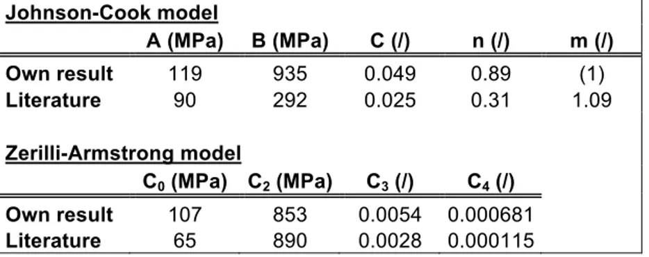
TABLE III. PARAMETERS DETERMINED FOR THE JOHNSON-COOK AND ZERILLI-ARMSTRONG STRENGTH MODELS.

Johnson-Cook model A (MPa) B (MPa) C (/) n (/) m (/) Own result 119 935 0.049 0.89 (1) Literature 90 292 0.025 0.31 1.09 Zerilli-Armstrong model C0 (MPa) C2 (MPa) C3 (/) C4 (/) Own result 107 853 0.0054 0.000681 Literature 65 890 0.0028 0.000115 NUMERICAL MODELING Introduction

As the experimental ballistic testing had shown that the piezoelectric transducer systematically gave larger values for the peak pressures than the crusher method, concerns were raised on the validity of the conversion table for the copper crushers used to convert the final length of the copper crusher into a peak pressure reached inside the chamber. More specifically, the question was raised if a supposedly quasi-static calibration of the conversion table could lead to the observed difference between the Kistler transducer and the crusher method by neglecting the strain rate sensitivity of the crusher material.

In order to evaluate this possible default in the conversion table, a numerical reverse engineering experiment was designed where in a finite element model the pressure impulse measured by the Kistler transducer was applied to a copper crusher. The as such in the numerical experiment obtained permanent deformation of the crusher Δlsim could then be compared to the reference permanent deformation Δlref corresponding to the initially applied peak pressure Ppeak (using the conversion table), and to the experimentally obtained average residual deformation Δlexp. If the simulated permanent deformation corresponded to the reference permanent deformation, the conversion table could assumed to be correct; if on the other hand it corresponded to the experimentally obtained permanent deformation (using the crusher method), the conversion table had not been calibrated correctly.

This reverse engineering experiment was done for all three powder masses used for the experimental ballistic testing of the second series (12 g, 14 g, 16 g).

Numerical setup

All finite element modeling was done in the explicit ANSYS Autodyn code [14]. Although originally the idea was to model both the piston and the crusher, and to apply the experimentally measured pressure curve (obtained with the Kistler transducer) to the free end of the piston, the following problems were encountered:

• Autodyn did not permit to introduce the measured pressure curve as an externally applied pressure, but only as an internally applied pressure. Applying the measured curve in this way to the piston however lead to

numerical inconsistencies. This problem was circumvented by applying the pressure directly onto the free end of the crusher (and hence discarding the piston from the finite element model), taking into account the relative contact surfaces of the piston and the sample (pressure acting on the free end of the crusher Pcrusher versus the peak pressure Ppeak acting on the free end of the piston).

• Autodyn did not allow introducing the real measured curve, but only allowed for either a rectangular pulse or a triangular pulse to be applied to the free end of the crusher. This problem was solved by applying a triangular pulse to the crusher with a maximum pressure corresponding to the experimentally measured peak pressure, and by adapting the length of the pulse Δt to have the same impulse in the numerical case as in the experimental case.

The different values for Pcrusher and Δt are given in Table IV.

The crusher was modeled using a Lagrangian mesh and implementing the previously fitted Johnson-Cook model as the strength model. The equation of state and failure model (although no failure was assumed to occur based on the experimental observations) were obtained from the material models for OFHC copper, as available in the Autodyn material library. The nominal dimensions of the crusher were used in the numerical model (height 4.9 mm and diameter 3 mm). A mesh sensitivity analysis was also performed in order to validate that the chosen spatial resolution gave satisfactory results.

Results and discussion

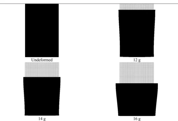
Figure 5 shows the final deformation of the copper crusher as a function of the powder mass. With increasing powder mass, the residual deformation increases as well, as expected. Similar to the real deformed samples, the copper crushers are deformed more on the side where the pressure was applied.

From Table IV it is clear that the simulated residual deformations correspond better to the reference deformations than to the average experimental deformations. This shows that the conversion table is valid for dynamic compression and that the aforementioned hypothesis that the conversion table was at the origin of the observed differences between the transducer and crusher measurements is not valid. As to obtain further proof for this, the simulations were repeated with an adapted Johnson-Cook model (with the C parameter equal to zero) corresponding to a rate-insensitive model fitted for quasi-static deformation. The hence obtained shapes of the deformed crusher as a function of powder mass were quasi-identical to the shapes shown in Figure 5. The calculated permanent deformations were also very similar to the deformations obtained with the rate-sensitive model, as illustrated in Table V, further strengthening the proof that the conversion table for this particular crusher material, even if possibly calibrated using quasi-static loadings, has been correctly calibrated.

TABLE IV. COMPARISON BETWEEN REFERENCE, SIMULATED AND EXPERIMENTAL PERMANENT DEFORMATION.

Powder mass (g) Ppeak (MPa) Pcrusher (MPa) Δt (µs) Δlref (mm) Δlsim (mm) Δlexp (mm)

12 159.2 270.4 991 0.69 0.56 0.49

14 251.5 427.2 709 1.35 1.35 1.12

16 319.6 542.9 678 1.80 1.92 1.59

Undeformed 12 g

14 g 16 g

Figure 5. Simulation results of the deformation of the copper crusher as a function of powder mass.

TABLE V. COMPARISON SIMULATED PERMANENT DEFORMATION BETWEEN RATE-SENSITIVE AND RATE-INSENSITIVE MODEL.

Powder mass (g) Δlsim,rate-sensitive (mm) Δlsim,rate-insensitive (mm) Relative difference (%)

12 0.56 0.55 2

14 1.35 1.29 4

16 1.92 1.86 3

COMPARISON AND DISCUSSION

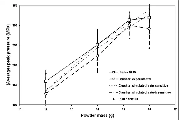
Figure 6 shows an overview of all the experimental data and simulated results. Error bars were added to the experimental data corresponding to twice the standard deviation, as is custom in error analysis. It is clear that statistically none of the three experimental techniques gives a statistically significant different result. As such, no definitive decision can be made on what technique (C.I.P., SAAMI or crusher) is the most or the least accurate.

The simulated crusher results neither permit to invalidate the experimental crusher results, as the conversion table used to convert the permanent deformation into peak pressure seems to be correct, independently of the fact if it was calibrated using dynamic or quasi-static loadings.

However, an important simplification that has been made in the numerical modeling is the discarding of the steel piston. If the rise time to reach peak pressure of the pressure wave send into the piston due to the deflagration of the powder inside the chamber would be sufficiently short, equilibrium conditions might not be reached in the piston. In that case, uniform acceleration of the piston can no longer be assumed and the transfer of the pressure wave from the steel piston to the copper crusher might be a wave propagation phenomenon. Partial reflection of the incoming pressure wave on the steel-copper interface (due to the differences in acoustic impedances) might then explain the lower stress experienced by the copper crusher. Additional numerical modeling has been started to elucidate on this possible wave phenomenon, but has so far not given any conclusive results.

Figure 6. Comparison of all experimental and simulation data.

CONCLUSIONS

The aim of this study was to compare copper crusher measurements with the C.I.P. and SAAMI piezoelectric measurements in order to elucidate on the typical measurement differences one can find between the results of not only crusher and piezoelectric measurements, but also between the different piezoelectric measurement techniques.

The copper crusher results were firstly compared to the piezoelectric transducers pressure measurements. Results of the study showed that although there was an

agreement in the pressure-time curves given by the two ballistic transducers, there were nevertheless some significant differences in the peak pressures measured with the three techniques.

In the case of the copper crusher, this difference might have been related to the dynamic behavior of the copper crusher gauge. The dynamic behavior of the copper crusher was hence measured for different dynamic strain rates using the Split Hopkinson Pressure bars setup (SHPB). The Johnson-Cook model was preferred to the Zerilli-Armstrong model as a strength model for the copper crusher material. However, comparison of the results of the following finite element modeling with the calibration table and the measured values permitted to conclude that the results of the crusher gauge were almost independent of the dynamic properties of the crusher material. When compared to the values obtained by the numerical model, the conversion table values given by the supplier can be considered as sufficiently accurate.

Taking into account the dispersion on the experimental data obtained with the three different measurement techniques, the copper crusher measurements and simulations did not permit to judge the accuracy of the different measurement techniques, nor to explain the typical differences in results obtained with the different methods.

Further numerical modeling is currently being carried out in order to evaluate the influence of the steel piston on the copper crusher response.

REFERENCES

1. 2005, “Pressure Measurement By Crusher Gauges Nato Approved Tests For Crusher Gauges”, AEP-23 Ed. 2, NATO Standardization Agency, NATO.

2. 1997, “NATO Piezo Gauge Replacement Programme”, AC/225(LG/3-SG/1)D/3(Rev.), NATO. 3. 2004, “COMBINATION ELECTRONIC PRESSURE, VELOCITY AND ACTION TIME

(EPVAT) TEST PROCEDURE”, PFP(NAAG-LG/3-SG/1)D1 Ch. 12, NATO.

4. 2011, “Edition Synthétique des decisions C.I.P. en vigueur”, Bureau Permanent C.I.P., Brussels, Belgium.

5. SAAMI/ANSI standards, SAAMI Technical Committee, available at http://www.saami.org, last accessed 30 November 2012.

6. National Instruments LabVIEW, http://www.ni.com/labview/, last accessed 30 November 2012. 7. Zerilli, F., and Armstrong, R., 1990, “Description of tantalum deformation behavior by dislocation

mechanics based constitutive relations”, J. Appl. Phys., 68, pp. 1580-1591.

8. Johnson, G. R., and Cook, W. H., 1983, “A Constitutive Model and Data for Metals Subjected to Large Strains, High Strain Rates and High Temperatures”, Proceedings of the 7th International Symposium on Ballistics, The Hague, The Netherlands, pp. 541-547.

9. Kolsky, H., 1949, “An Investigation of the Mechanical Properties of Materials at Very High Loading Rates”, Proc. Phys. Soc. London, B62, pp. 676.

10. Hopkinson, B., 1914, “A Method of Measuring the Pressure Produced in the Detonation of High Explosives or by the Impact of Bullets”, Roy. Soc. Phil. Trans., A213, pp. 437-456.

11. Meyers, M., 1994, “Dynamic Behavior of Materials”, John Wiley & Sons Inc, New York, USA. 12. Bai, Y., and Dodd, B., 1992, “Adiabatic Shear Localization”, Pergamon Press, UK.

13. Banerjee, B., 2005, “An evaluation of plastic flow stress models for the simulation of high-temperature and high-strain-rate deformation of metals”, Dept. of Mechanical Engineering, University of Utah, USA.