A
COMPARISON OF WITHIN
-
SEASON YIELD PREDICTION ALGORITHMS
1
BASED ON CROP MODEL BEHAVIOUR ANALYSIS
2 3
Dumont B.1*, Basso B.2, Leemans V.1, Bodson B.3, Destain J.-P.3, Destain M.-F.1
4 5
1, ULg Gembloux Agro-Bio Tech, Dept. Environmental Sciences and Technologies, 5030 Gembloux, Belgium 6
2, Dept. Geological Sciences, Michigan State University, East Lansing, MI, USA 7
3, ULg Gembloux Agro-Bio Tech, Dept. Agronomical Sciences, 5030 Gembloux, Belgium 8
* Corresponding author: 2 Passage des Déportés, 5030 Gembloux, Belgium 9 Email: [email protected], 10 Tel: +32(0)81/62.21.63, fax: +32(0)81/62.21.67 11 12
Keywords: STICS crop model, Climate variability, LARS-WG, Yield prediction, Log-normal 13
distribution, Convergence in Law Theorem, Central Limit Theorem.
14 15
Abstract 16
The development of methodologies for predicting crop yield, in real-time and in 17
response to different agro-climatic conditions, could help to improve the farm management 18
decision process by providing an analysis of expected yields in relation to the costs of 19
investment in particular practices. Based on the use of crop models, this paper compares the 20
ability of two methodologies to predict wheat yield (Triticum aestivum L.), one based on 21
stochastically generated climatic data and the other on mean climate data. 22
It was shown that the numerical-experimental yield distribution could be considered as 23
a log-normal distribution. This function is representative of the overall model behaviour. The 24
lack of statistical differences between the numerical realisations and the logistic curve showed 25
in turn that the Generalised Central Limit Theorem (GCLT) was applicable to our case study. 26
In addition, the predictions obtained using both climatic inputs were found to be 27
similar at the inter- and intra-annual time-steps, with the root mean square and normalised 28
deviation values below an acceptable level of 10% in 90% of the climatic situations. The 29
predictive observed lead-times were also similar for both approaches. Given (i) the 30
mathematical formulation of crop models, (ii) the applicability of the CLT and GLTC to the 31
climatic inputs and model outputs, respectively, and (iii) the equivalence of the predictive 32
abilities, it could be concluded that the two methodologies were equally valid in terms of 33
yield prediction. These observations indicated that the Convergence in Law Theorem was 34
applicable in this case study. 35
For purely predictive purposes, the findings favoured an algorithm based on a mean 36
climate approach, which needed far less time (by 300-fold) to run and converge on same 37
predictive lead-time than the stochastic approach. 38
A
COMPARISON OF WITHIN
-
SEASON YIELD PREDICTION ALGORITHMS
39
BASED ON CROP MODEL BEHAVIOUR ANALYSIS
40 41
1.
Introduction
42
Agricultural production is greatly affected by variability in weather (Semenov et al., 43
2009; Supit et al., 2012). Providing an opportunity to study the effects of variable inputs (such 44
as weather events) on harvestable crop parts, crop models have been used successfully to 45
support the decision-making process in agriculture (Basso et al., 2011; Ewert et al., 2011; 46
Thorp et al., 2008). The development of methodologies for predicting grain yield, in real time 47
and in response to different agro-climatic conditions (Dumont et al., 2014b; Lawless and 48
Semenov, 2005), would further improve farm management decisions by providing an analysis 49
of the trade-off between the value of expected crop yields and the cost of inputs. 50
Plant growth and development can be seen as systems linked to the environment in 51
linear and non-linear ways (Campbell and Norman, 1989; Semenov and Porter, 1995). Many 52
of the links between crop dynamics and atmospheric variables are non-linear and 53
interdependent. Crop models were developed about 40 years ago as an effective substitute for 54
ambiguous and cumbersome field experimentation (Sinclair and Seligman, 1996). The greater 55
expectations from modelling rapidly led to increasingly detailed descriptions of the 56
functioning of the biotic and abiotic components of cropping systems, leading to an increase 57
in complexity and computer sophistication. Crop models provide the best-known approach for 58
improving our understanding of complex plant processes as influenced by pedo-climatic and 59
management conditions (Semenov et al., 2007), and they have proved to be more heuristic 60
tools than simply a substitute for reality (Sinclair and Seligman, 1996). Most physically based 61
soil-crop models operate on a daily time basis and simulate the evolution of variables of 62
interest through daily dynamic accumulation. 63
In crop models, weather conditions need to be described as accurately as possible. 64
Weather data are the input data that drive the model and daily crop growth. It has been shown 65
that weather data have a greater effect on yield than technical data and soil parameterisation 66
(Nonhebel, 1994). In addition, crop model predictions (such as phenological development, 67
biomass growth, or yield elaboration) are affected by temporal fluctuations in temperature 68
and/or precipitation, even when the mean values remain similar (Semenov and Porter, 1995). 69
It has been demonstrated that historical mean weather data might be inappropriate for 70
predicting crop growth because of the non-linear response of crops to agro-environmental 71
conditions (Porter and Semenov, 1999, 2005; Semenov and Porter, 1995). The sequencing of 72
weather events greatly affects dynamic crop simulations; interactive stresses might have a 73
greater impact on the final value of crop characteristics of interest (such as grain yield) than 74
individual stresses (Riha et al., 1996). 75
Important research has been done on estimating the form of historical crop yield 76
distributions. Day (1965) analysed crop yield distributions using the Pearson System and 77
found that: (i) crop yield distribution is generally non-normal and non-log-normal, whereas 78
(ii) the skewness and kurtosis of yield distribution (the mathematical third and fourth central 79
moment, respectively) depend on the specific crop and the amount of available nutrients. His 80
conclusions were corroborated by Du et al. (2012), who considered that the development of a 81
complete theory on the effect of input constraints on yield skewness required empirical 82
studies on diverse crops grown in different production environments. Several authors (Just 83
and Weninger, 1999; Ramirez et al., 2001) have tried to assess the normality of crop yield 84
distribution, but have not been able to do so. Just and Weninger (1999) identified three 85
specific reasons for this: (i) the misspecification of the non-random components of yield 86
distributions, (ii) the misreporting of statistical significance, and (iii) the use of aggregate 87
time-series data to represent farm-level yield distributions. Numerous works have referred to 88
the ‘usual left-tail problem’, which deals with the low probability of occurrence of some very 89
low yields, characterised by particularly poor climate conditions (Hennessy, 2009a). More 90
recently, Hennessy (2009a, b, 2011) analysed crop yield expectations with reference to the 91
Law of the Minimum Technology and the Law of Large Number. 92
Within the context of yield prediction, there is a distinction between statistical models 93
and process-based models. In the early 1960s the National Agricultural Statistics Service 94
(NASS) of the United States Department of Agriculture (USDA) developed a method for 95
assessing crop yield based on several sources of information, including various types of 96
surveys and field-level measurements. These yield forecasting models are based on analysing 97
relationships of samples at the same stage of maturity in comparable months over the 98
preceding 4 years (Allen et al., 1994; Keller and Wigton, 2003). More recently, the statistical 99
models have been coupled with remote data and recorded climatic measurements covering a 100
preliminary period of a few months (Doraiswamy et al., 2007). As the yield prediction model 101
is empirical and not physically based, this approach has serious limitations: (i) the future 102
impact of past stress effects is not integrated into the physiological plant growth and (ii) the 103
compensation mechanisms of crop management are not fully considered. 104
Process-based crop model approaches appear to be better alternatives for yield 105
prediction, but crop models should rely on data that reflect hypothetical future scenarios. An 106
appropriate and sophisticated approach for predicting grain yield with incomplete weather 107
data was described by Lawless and Semenov (2005). It is based on the use of the Sirius crop 108
simulation model (Jamieson et al., 1998; Semenov et al., 2007; Semenov et al., 2009) and the 109
LARS-WG stochastic weather generator (WG) (Racsko et al., 1991; Semenov and Barrow, 110
1997). The methodology for predicting grain yield with incomplete weather data was related 111
to the crop’s life cycle: based on observed weather for the first part of the growing season, the 112
authors used a stochastic WG to produce a probabilistic ensemble of synthetic weather time-113
series for the remainder of the season. WGs can be used to generate multiple stochastic 114
realizations of extended sequences of real historical weather data (Lawless and Semenov, 115
2005; Mavromatis and Hansen, 2001; Mavromatis and Jones, 1998; Singh and Thornton, 116
1992), allowing risk assessment studies to be performed. The weather time-series built in this 117
way were then used as an input in a crop simulation model to generate distributions of crop 118
characteristics (such as phenological stages, end-season grain yields). As the season 119
progressed, the uncertainty of the crop simulations decreased. This approach is interesting, but 120
time-consuming and machine intensive. 121
Another method would involve replacing future data by forecasted weather. The initial 122
problems here, though, are that forecasting has a time limit and that forecast accuracy 123
diminishes with the long-time predictions. An added problem is the need to downscale data 124
from a Global or Regional Climate Model (GCM/RCM) to local conditions at a resolution 125
suitable for crop simulation models. The EU-funded DEMETER and ENSEMBLES projects 126
are probably the two most representative examples of this application in Europe (Cantelaube 127
and Terres, 2005; Challinor et al., 2005; Hewitt, 2004; Palmer et al., 2005). It is worth 128
mentioning that GCM/RCM downscaling can be achieved by linking a seasonal forecast with 129
a WG (Semenov and Doblas-Reyes, 2007), which allows yield prediction to be performed. It 130
has been shown, however, that this approach is not any better at yield prediction than the 131
approach based on historical climatology (Semenov and Doblas-Reyes, 2007). 132
Dumont et al. (2014b) have developed a similar approach. They assessed the potential 133
of overcoming the lack of future weather data by using seasonal averages. For each of the 134
climatic variables necessary to run the crop model (temperature, precipitation, solar radiation, 135
vapour pressure, wind speed), they computed the seasonal averages as the daily mean values 136
calculated from a 30-year historical weather database. Being based on only one future 137
projection, it was very light in terms of computational requirement. 138
The aim of our study was to compare the efficiency of two crop yield prediction 139
methodologies that are based only on historical records. To make the yield predictions, the 140
Lawless and Semenov (2005) approach, based on using a high number of stochastically 141
generated climate data, and the Dumont et al. (2014b) methodology, based on using seasonal 142
averages, were selected. Both approaches benefit from the same amount of realized 143
information. In each of the studies, relevant yield predictions could be made only at a late 144
stage, but no research had ever compared the methodologies in an identical case study or 145
using the same crop model. Comparing the efficiency of the two methodologies relied on an 146
in-depth analysis of crop model behaviour based on a sound statistical foundation. The 147
research findings reported by Day (1965) and Hennessy (2009a, 2009b, 2011) were applied to 148
our study of crop model behaviour and the mathematical nature of the computed weather 149
time-series is discussed in relation to the Convergence in Law Theorem and Central Limit 150
Theorem (CLT). 151
2.
Material and methods
152
2.1
Overview of the procedure
153
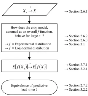
To answer the question of whether the predictive approaches have equal potential in 154
terms of their ability to predict yield with the same accuracy and lead-time, we developed a 155
four-step procedure (see Figure 1). The first step focused on the applicability of the CLT to 156
the weather input generation. In other words, it has to be verified that the stochastically 157
generated climates used by Lawless and Semenov (2005), denoted Xn, converged on the mean
158
climate computed by Dumont et al. (2014b), denoted as X. This was ensured by the properties 159
of the LARS-WG, and was thus only reminded in the material and method section. 160
The second step sought to determine if the crop model answers (i.e., in this case, the 161
simulated end-season grain yields) could be approximated by a general function ‘f’ being 162
representative of the whole model and linking the climatic inputs and the simulated variable 163
output. The numerical-experimental crop yield distributions obtained with stochastically 164
generated climate data were analysed. In compliance with the Generalised Central Limit 165
Theorem (GCLT), the approximation of the simulated yield distribution by a log-normal 166
distribution was assessed. 167
In the third step, which was divided into two successive phases, the simulations 168
obtained using both sets of climatic data were compared. In the first phase, the within-season 169
yield predictions were compared on an annual basis. In the second phase, the corresponding 170
predictive lead-times were compared. If the two approaches were found to be equivalent (i.e., 171
if the mathematical expectation of the Lawless and Semenov [2005] approach, denoted as 172
E[f(Xn)], did not differ significantly from the other approach, where the mathematical
173
expectation of the outcomes was denoted E[f(X)]) this would validate the applicability of the 174
Convergence in Law Theorem. 175
2.2
Case study
176
The data used in this paper are derived from an experiment conducted to study the 177
growth response of wheat (Triticum aestivum L., cultivar Julius) in the agro-environmental 178
conditions of the Hesbaye region in Belgium. The soil at the experimental site was a classic 179
loam type. 180
Biomass growth was monitored over 3 years (crop seasons 2008-09, 2009-10 and 181
2010-11). In 2008-09, the yields were fairly high under adequate nitrogen fertiliser rates, due 182
mainly to good weather conditions. In the 2009-10 and 2010-11 seasons, there was severe 183
water stress, resulting in yield losses. In 2009-10 the water stress occurred in early spring and 184
early June; in 2010-11 it occurred from February to the beginning of June. In the summer 185
rainfall returned, ensuring a normal growth rate for the last part of the season. Reasonable 186
grain yield levels were achieved, but the straw yield remained low, giving a high harvest 187
index. 188
The current practice in Belgium is to apply a total of 180 kgN.ha-1 in three equal 189
fractions (60 kgN.ha-1) at the tiller, stem extension and flag-leaf stages, which is known to be 190
close to the optimum nitrogen rate for crop growth under the climatic conditions prevalent in 191
the country (Dumont et al., 2014a). Over the 3-year experiment, at this fertilisation level, the 192
grain yields reached 12.6, 7.8 and 7.1 ton.ha-1 of dry matter, respectively Among the 193
replicates, the highest yield was 14.0 ton.ha-1 in 2009 and the lowest was 5.8 ton.ha-1 in 2011. 194
2.3
Modelling crop growth
195
2.3.1
The STICS crop model
196
The STICS crop growth model (Brisson et al., 2003; Brisson et al., 2009; Brisson et 197
al., 1998) was used to simulate the end-season grain yields (expressed in tons of dry matter 198
per hectare [ton.ha-1]) that were the focus of the study. In this model, dry matter is related to 199
absorbed radiation according to the radiation-use efficiency (RUE) concept (Monteith and 200
Moss, 1977). STICS allows the effect of water and nutrient stress on development rate 201
(Palosuo et al., 2011) to be taken into account The actual and potential evapotranspiration 202
were computed using the Penman formalism (Penman, 1948). The STICS model requires 203
daily weather inputs (i.e., minimum and maximum temperatures, total radiation and total 204
rainfall, vapour pressure and wind speed). 205
The STICS model parameterisation, calibration and validation were performed on the 206
3-year database used for the case study. For the calibration process, the DREAM(-ZS) 207
algorithm (Dumont et al., 2014c; Vrugt et al., 2009) was used. The highly contrasting climatic 208
data in the 3-year database were used to parameterise crop water, thermal and nitrogen stress 209
dependence. Times-series of leaf area index (LAI) measurements (once a month), biomass 210
and grain yield estimates (once a fortnight and at the time of final grain yield), soil N-NO3 -211
and N-NH4+ (once a fortnight) and plant N uptake (once a month) were used to parameterize 212
the various aspects of plant development (i.e., grain yield components, plant growth rate, soil 213
water and nitrogen uptake). There is more detail on the model calibration process and the 214
accuracy of the model in Dumont et al. (2014c). 215
2.3.2
The simulation process
216
It was assumed that cultivar, soil and management remained the same for all 217
simulations, and therefore that the simulations differed only in terms of weather inputs. In 218
order to ensure that the simulated plant growth would be limited only by climatic factors, 219
simulations were conducted with adequate nitrogen fertilisation levels. The simulated 220
fertiliser rate used for the study was a total of 180 kgN.ha-1 applied in three equivalent 221
fractions (60 kgN.ha-1) at the tiller, stem extension and flag-leaf stages. 222
In order to simplify the simulation process, the same management techniques were 223
applied to each simulation, following the 2008-09 itinerary. The sowing date was in late 224
October, on 10/25.. Each simulation was run with the sowing date as the starting point. The 225
same soil description was used for all simulations. The soil-water content was initialized at 226
field capacity, and the soil initial inorganic N content corresponded to real measurements 227
taken in the first year of the experiments. The three 60 kgN.ha-1 nitrogen fertilizer doses were 228
applied at fixed dates (i.e., at the tillering, stem extension and flag-leaf stages in 2008-09) on 229
on the 03/23, 04/16 and 05/25, respectively. 230
2.4
Weather database generation
231
2.4.1
Historical climatic database
232The complete 30-year (1980-2009) Ernage weather database (WDB) was used in this 233
study to generate the crop model inputs. Part of Belgium’s Royal Meteorological Institute 234
(RMI), the Ernage weather station is 2 km from the experimental field. The measurements 235
carried out by the station involved all the climatic variables required to run a crop model. 236
2.4.2
Generating a probabilistic ensemble of synthetic weather data
237
The first approach used for within-season yield predictions was based on the work of 238
Lawless and Semenov (2005). In essence, the 30-year Ernage WDB was analysed using the 239
LARS-WG, which computed a set of parameters representing the experimental site (daily 240
mean values, daily standard deviations, daily maxima and minima, successive wet and dry 241
series and frequency of rainfall events). They the LARS-WG can be used to generate a set of 242
stochastic synthetic weather time-series representative of the climatic conditions in the area. 243
According to Lawless and Semenov (2005), and for reasons detailed at section 2.6.1, 300 244
time-series were generated and then input into the model. 245
Using a WG is an appropriate way of simulating yields under new combinations of 246
probable weather scenarios. If the crop model is correctly calibrated and validated, this would 247
lead to a simulation of stress conditions not observed during the limited time of a field 248
experiment. 249
2.4.3
Generating the mean climate data
250
The second approach, based on the work of Dumont et al. (2014b), used a daily mean 251
climate dataset. The dataset was drawn from the Ernage WDB, and the daily mean data for 252
each climate variable was computed. In other words, for each variable and day, each element 253
of the mean climate matrix was computed as the mean of the corresponding 30 values of the 254
same day over the 30 years. 255
This approach relies on the strong assumption that climate conditions are very close to 256
the seasonal norms. This is particularly the case with precipitation, for which a minimum 257
value is thus available each day, ensuring reduced water stress. As discussed by Dumont et al. 258
(2014b), such an assumption leads to simulations that, at any time of the year, show the 259
remaining yield potential. Other assumptions and limitations of this approach are described by 260
Dumont et al. (2014b). 261
2.4.4
Within-season prediction
262
These two types of synthetic weather data were used to perform within-season yield 263
prediction. Climate series were generated from recorded historical climatic data. At a pre-264
determined rate (e.g., every 10 days), the observed weather sequences were replaced by either 265
the probabilistic ensemble of synthetic climatic time-series or the mean climatic data. The 266
climatic matrix ensembles of data thus generated could then be used as inputs for the crop 267
growth model. The effect of such probable climatic conditions could be studied for the 268
various yield components. With this methodology, the proportion of the hypothetical future 269
data diminished as the growing season progressed, as did the uncertainty about the 270
corresponding simulated yield. 271
2.5
Statistical considerations
272
2.5.1
The Convergence in Law Theorem
273
The convergence in law (→L) or in distribution (→d) is considered to be one of the
274
weaker laws of convergence, but underpins the demonstration of many theorems and is key to 275
our analysis of crop model behaviour. It can be enunciated as follows: Let {Xn} be a sequence
276
of n random variables x and let X be a random variable. Denote by Fn(x) the distribution
277
function of Xn for all real x. The convergence in law theorem then states that {Xn} converges in
278
distribution to X ( Xn →d X) as n→∞, if there is a function f, which extends over the real space
279
(R→R), continuous and bounded such that: 280
( )
[
f X]
E[
f( )
X]
E n → (Eq. 1) 281 2822.5.2
The Central Limit Theorem and the log-normal distribution
283
The Central Limit Theorem (CLT) (de Moivre, 1976) can be enunciated as follows: 284
Let {Yn} be independent random variables, of the same law (i.e., identically distributed), of
285
integrable square. We denote µ its expectation and σ² its finite variance; here we assume that 286 σ²>0. Then: 287 , Y n S n L n → −µ σ as n→∞ (Eq. 2) 288
where Sn is the sum of the Yn values. Y follows a Gaussian distribution, centred in zero, with
variance one: Y~
N
N
N
N
(0,1). In practical terms, the CLT implies that for ‘large’ n, the distribution 290of Yn may be approximated by a Normal distribution with mean µ and variance σ²/n.
291
The CLT allows for different generalisations in order to ensure the convergence of a 292
sum of random variables under a weaker hypothesis (particularly with regard to the 293
distribution from which they originated), but relies on conditions that ensure that no variable 294
has significantly greater influence than any other variable. In particular, the CLT has been 295
extended to the product of functions, the logarithm of a product being the sum of the 296
logarithms of each factor. This extension is known as the Generalised Central Limit Theorem 297
(GCLT). 298
Day (1965) suggested assessing the following generalised log-normal transformation 299
of data in order to determine if crop yields Yn responded to a log-normal distribution:
300
(
max)
maxlog lnY Y , Y Y
Yn− = − n n < (Eq. 3)
301
where Ymax corresponded to a theoretical maximal threshold and Yi, i ϵ {1,...,n} corresponded to
302
the observed yield under given climate Xi, in other words Yi=f(Xi).
303
An easy way to assess the log-normal behaviour of a yield sampling Yn is to evaluate
304
the normality of the corresponding normalised and zero-centred log-transform vector YNorm
305
(computed according to Eq. 3). Such an evaluation relies on the use of the Kolmogorov-306
Smirnov test (Dagnelie, 2011; Feller, 1948). The vector of observations Yn could therefore be
307
transformed according to Eqs. 2 and 3, leading to Eq. 4 where the corresponding distribution 308
(Eq. 5) is assumed to follow the log-normal distribution. 309
(
)
( ) ( n) n Y Y Y Y n Norm Y Y Y − − − − = max max ln ln max lnσ
µ
(Eq. 4) 310(
)
( )(
)
( ) ( ) − − − − = − − − 2 ln ln max ln max max max max ln . 2 1 exp . . ln . 2 1 ) ( y Y y Y y Y y Y y Y y pσ
µ
σ
π
(Eq. 5) 311 3122.6
Practical implementation of the statistical basis of general model behaviour
313
assessment
314
2.6.1
LARS-WG and mean climate data
315
The LARS-WG was specifically designed “to generate synthetic data which have the 316
same statistical characteristics as the observed weather data” (Semenov and Barrow, 2002). It 317
is therefore clear that the CLT applies to the inputs, ensuring that the stochastically generated 318
climatic time-series (Xn) used in the Lawless and Semenov (2005) methodology converge in
319
law with the mean climatic data (X) proposed by Dumont et al. (2014b). The statement Xn →L
320
X, however, does not say how large n must be for the approximation to be practically useful. 321
Lawless and Semenov (2005) demonstrated that a set of 60 synthetic weather time-series was 322
enough to achieve a stationary prediction of mean grain yield. As the stochastic component of 323
LARS-WG is driven by a random seed number, however, Lawless and Semenov (2005) 324
recommended using at least 300 stochastically generated weather time-series, which latter 325
was therefore the number of time-series used to conduct this research. 326
2.6.2
Hypothesis underlying the GCLT
327
Crop models are known to have a non-linear response to weather conditions. They also 328
have limitation factors affecting yield components, attributable mainly to genetic 329
specification, such as a maximum number of grains in place or a maximal weight of 330
individual grains. A third feature of crop models is that, within them, growth is simulated as a 331
differential daily increment (Eq. 6) and that most of the increment (f(Y(t), X(t), θ)) is 332
determined by functions that are themselves either multiplicative (e.g., growth function x 333
stress function) or hierarchical (e.g,. biomass growth being exponentially connected to LAI 334 value). 335
(
t t) ( )
Y t f(
Y( ) ( )
t ,X t ,θ
)
Y +∆ = + (Eq. 6) 336where Y(t) and Y(t+∆t) are the outputs simulated at the daily ∆t time step, X(t) is the vector of 337
input variables, θ is the vector of model parameters and f accounts for the simulated model 338
processes. 339
We can reasonably assume that each simulated end-season yield (i.e., Yn) is the result
340
of a unique combination of climatic variables Xn: different combinations of variables (e.g.,
341
temperature, vapour pressure); different dynamics over the seasons for each individual 342
variable (stochastic generation of values such as X(t), X(t+1), X(t+2) and so on); and different 343
dynamics of interacting variables (successive dry and wet series). To some extent, this ensures 344
that the simulated yields are independent random variables, which is a necessary condition for 345
assessing CLT applicability. 346
The second assumption is that the output variables have the same law. The objective of 347
the second step of the procedure is to find this general law and validate the CLT applicability 348
to the model outputs. Some discussions, however, have to be made at this stage. Each input 349
variable Xn (known to comply with the CLT) is used to pilot the simulations through the same
350
complex model summarized as Eq. 6. The sum term in Eq. 6, which constitutes the daily 351
increment, is therefore also consistent with the CLT. On the other hand, due to the structure of 352
a crop model, it is known that under the f(Y(t), X(t), θ) term there are hidden hierarchical (Y = 353
f (X) ≡ g(h(X)) and multiplicative (Y = f(X) ≡ g(X)×h(X)) functions. The model f(Y(t), X(t), θ) 354
remains the same for all assessed input variables. Provided that none of the climatic variables 355
has a significantly greater influence than others, the main objective is therefore to determine if 356
the generated outputs respond to a unique distribution law compliant with the CLT. 357
2.6.3
The log-transformation of simulated outputs to assess the GCLT
358
Among the generalisations of log-transformation proposed by Day (1965), the one 359
proposed at Eq. 3 appeared suitable for the observed yield distributions and the ‘left-tail’ 360
problem. Day (1965) stated, however, that it would be difficult to find the threshold Ymax (Eq.
361
3)that would correspond to the potential maximal yield of the crop, for which the probability 362
of occurrence should be zero. 363
An easy, yet relevant, way to find the potential yield Ymax in Eqs. 3 to 5 would be to
364
consider that the maximal yield obtained under n climatic scenarios generated with LARS-365
WG was the upper limit of the distribution. The probability that such an optimal climatic 366
scenario had occurred would be quite low (close to zero) and due exclusively to a particular 367
combination of climatic variables resulting from the stochastic generation performed using 368
LARS-WG. 369
2.7
Comparisons of model output distributions and yield prediction abilities
370
The third and fourth steps of the procedure focus on comparing the distribution of the 371
simulated grain yields obtained using the Lawless and Semenov (2005) methodology with the 372
results obtained using the Dumont et al. (2014b) approach. As a high number of synthetic 373
climate data was used, and provided that a general law f can be highlighted, the mathematical 374
expectation of the end-season yields (i.e., E[f(Xn)]) could be computed as its empirical mean.
375
It could then be compared with the unique yield value simulated, using mean climate as the 376
climatic projection (i.e., E[f(X)]). 377
There were three levels of comparison. First, the model was run on inputs consisting 378
only of stochastic climate data on the one hand and only of daily mean data on the other. The 379
end-season yield value obtained from the second dataset was positioned within the yield 380
distribution obtained from the first dataset. As the main aim of the study was to compare the 381
two within-season yield prediction algorithms, the equivalence of the yields simulated using 382
the two approaches would then be evaluated throughout the season (2.7.1). Finally, the 383
predictive lead-time for both approaches would then be compared (2.7.2). 384
2.7.1
Single year analysis and model output distributions
385In order to see if the two methodologies led to same output simulations, two statistical 386
criteria were used: relative root mean square error (RRMSE) and normalised deviation (ND) 387
(Eqs. 7 and 8). The two approaches would be considered as equivalent if the value of both 388
criteria was less than 10%. The 10% threshold was seen as appropriate for two reasons. First, 389
an ND value less than 10% is usually thought to validate model simulations (Beaudoin et al., 390
2008; Brisson et al., 2002). Second, the within-season predictive ability would be assessed 391
considering a plus or less 10% error around the final simulated grain yield (cfr 2.6.4 - 392 Analysed data). 393
(
)
( )
∑
∑
= = − = k i i k i i i Y k Y Y k RRMSE 1 1 2 1 ˆ 1, with expected RRMSE < 0.1 (Eq. 7)
394
( )
( )
( )
∑
∑
∑
= = = − = k i i k i i k i i Y k Y Y ND 1 1 1 1 ˆ, with expected ND < 0.1 (Eq. 8)
395
where Y and Ŷ refer to the end-season yields simulated using the two approaches and i refers 396
to the ith simulation of end-season yields performed during the season. 397
2.7.2
Inter-year analysis and prediction ability of the approaches
398The ability of both approaches to predict yield was assessed finally by comparing the 399
predictive lead-time curves observed for the original 30-years Ernage weather database. The 400
computation of the curves followed the process proposed by Lawless and Semenov (2005) 401
and consisted of plotting the cumulative probability distribution of the first day for which the 402
yield could have been predicted. There is more detail on how this distribution is computed in 403
Lawless and Semenov (2005) and Dumont et al (2014b). 404
With regard to the predictive ability of the model, the within-season predictive 405
simulations were compared to the simulated final grain yield, with an error of plus or minus 406
10% considered as an acceptable predictive value. There is more detail on this in the work 407
reported by Lawless and Semenov (2005) or Dumont et al. (2014b), 408
3.
Results
409
3.1
Assessing the crop model behaviour
410
3.1.1
Analysis of the experimental probability density function for purely
411synthetic climate data
412Figure 2 shows the probability density function and cumulative distribution function 413
of grain yield simulations conducted on purely synthetic climate data generated using the 414
LARS-WG. The simulated outputs were subjected to the log-normal distribution. The 415
log-normal distribution was not fitted to the data, but the theoretical distribution was 416
computed on the basis of the characteristic values of the simulated output that were the mean 417
and standard deviation of the log-transformed values (Eq. 5). The computed theoretical 418
function (solid black lines) matched the numerical-experimental distribution (solid grey line 419
or grey histogram) fairly well. The log-normal distribution therefore seemed particularly 420
suitable for representing the crop model answer. 421
Using this approach, it was possible to compute the mean (vertical black line in Fig. 422
2B) or median of the experimental distribution, intercepted at the 50th percentile (horizontal 423
black line in Fig. 2B), which was 11.25 ton.ha-1 and 11.82 ton.ha-1, respectively. From a 424
probabilistic point of view, at sowing there was a 50% chance of achieving at least 11.82 425
ton.ha-1, without any prior knowledge of the forthcoming weather. In comparison, the mean of 426
the distribution occurred at a probability level of 40%. The simulated yields accorded with the 427
observations performed during the original 3-year experiments, the values of which were 428
presented at section 2.2. 429
The yield simulated using the pure mean dataset was 12.14 ton.ha-1. In the previous 430
distribution this would have occurred at a probability level of 56%, implying that, if mean 431
climate data were used instead of stochastic data, there was a 16% chance of overestimating 432
the yields by about 7.5%. This latter value was computed as the relative difference between 433
the yield prediction obtained via the mean climatic projections (i.e., E[f(X)]) and that obtained 434
via the stochastic simulations (i.e., E[f(Xn)]).
435
With regard to the theoretical computed log-distribution, the cumulative distribution 436
function curve showed a left-tail, with a theoretical minimum value fixed at -∞, whereas the 437
minimum simulated grain yield was 3.4 ton.ha-1. The maximum simulated Ymax value was14.9
438
ton.ha-1. 439
Finally, the YNorm vector was computed according to Eq. 4 and its normality was
440
evaluated using the Kolmogorov-Smirnov test. The p-value was 0.837, far higher than the 441
expected value of 0.025 (= α/2). This led to the conclusion that the experimental distribution 442
could not be considered as differing from a log-normal function, and confirmed the validation 443
of the GCLT and its applicability to the crop model. In other words, the STICS crop model 444
could be considered as a global f-function that links the X(t) random climatic inputs and the 445
Y(t) simulated grain yield outputs. 446
3.1.2
Climate data combination and the log-normal behaviour
447
When performing within-season yield prediction using the Lawless and Semenov 448
(2005) approach, the stochastic projections were coupled with observed time-series. The issue 449
then was to determine to what extent (i.e., till which amount of observed weather data) the 450
crop model could exhibit a log-normal behaviour ? An example of the simulated grain yields 451
based on combined synthetic and observed data, and drawn from 300-year weather 452
simulations, was computed for the 1981-1982 crop season (see Fig. 3). Progressing through 453
the crop lifecycle, the uncertainty about the weather data lessened as the amount of observed 454
time-series increased. The surrounding bounds on corresponding yield predictions therefore 455
gradually tightened until a final value (11.6 t.ha-1) was reached with purely observed time-456
series. 457
For each section of data that could be extracted from this figure, an analysis conducted 458
as described in the previous section was performed. Table 1 shows the p-value resulting from 459
the Kolmogorov-Smirnov test, applied on the normalised vector of data (Eq. 4). The 30 years 460
of the database were studied individually, as year 1981-82 (Fig. 3), using a 10-day 461
replacement rate of the observed time-series. The p-value under the acceptable 0.025 (α/2, α = 462
5%) expected criteria are underlined in grey. Until the day of the year (DOY) 06/15, our 463
analyses showed that in almost 95% of cases the model could be considered as having log-464
normal behaviour. The test generally failed later in the season (between 06/15 and 08/24), 465
whatever the year. For example, the 1981-82 crop season (Fig. 3) failed the Kolmogorov-466
Smirnov test for DOY 06/15, when the p-value was 0.01, below the acceptable value of 0.025. 467
Figure 4 presents same results as Figure 2, but for 1981-82 and taking account of real 468
time-series observed until 06/15. The corresponding simulations (Fig. 3) showed that the 469
period between DOY 05/16 and 06/15 corresponded to a transient period where simulation 470
distribution evolved from widely spread to closely tightened around the final simulation 471
obtained only for real climate. At DOY 06/25 (Fig. 4), a p-value of 0.02 was obtained. The 472
distribution seemed closer than a normal/symmetric distribution, as confirmed by the 473
proximity of the mean and median of the distribution (Fig. 4B) 474
In conclusion, for most of the season (from sowing until DOY 06/15), the log-normal 475
distribution seemed able to account for crop yield distribution. This confirmed the 476
applicability of the GCLT. Later in the season, as the part represented by the observed time-477
series became dominant within the model inputs (at DOY 06/15, 230 days of real weather had 478
been observed), the log-normal behaviour disappeared. At that point, on one hand there was 479
no longer any independence of the climate series, and on the other hand the number of grains 480
was fixed. 481
3.2
Assessing the potential of yield prediction
482
3.2.1
Single-year analysis of model outputs
483The follow-up to the research focused on determining if the Converge in Law theorem 484
could be applied to STICS model simulations. Thus, the mathematical expectation of the 485
simulation conducted on 300 stochastic climate data (E(f[Xn])) was compared with the
486
simulation conducted using the mean climate data E(f[X]). 487
Figure 5 presents the variation in predicted model output during within-season 488
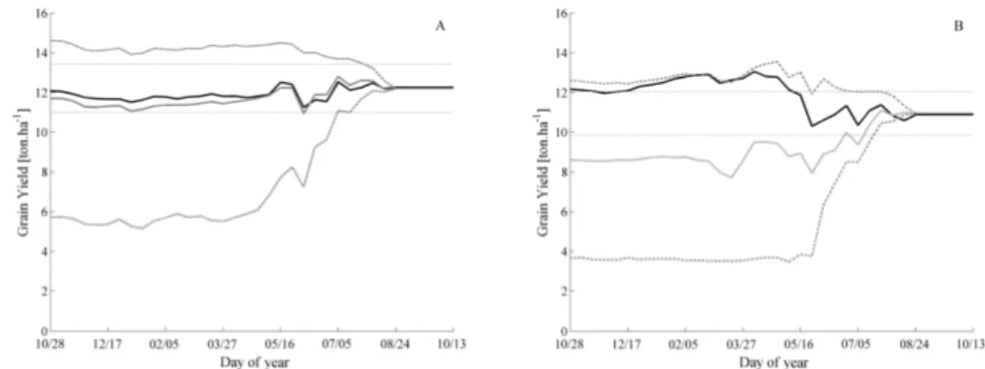
simulation, using the both Lawless and Semenov (2005) and Dumont et al. (2014b) 489
approaches. In terms of the outputs of the methodologies, there were contrasting results in the 490
1991-92 (Fig. 5A) and 2007-08 (Fig. 5B) seasons. Figure 5 is based on Figure 3, which 491
summarised the information using three characteristic values: the average and the percentile 492
2.5 and 97.5 of the 300 simulations. 493
For the 1991-92 season, the mean values of the 300 simulations (solid grey line) were 494
very close to the results generated using the Dumont et al. (2014b) approach (solid black 495
line). The RRMSE and ND values were 0.026 and -0.015, respectively. 496
This was not the case for the 2007-08 season. The main differences between the two 497
seasons could be explained by the first 10 days of the observed time-series (drastic autumn 498
conditions) for the crop seasons from 2005 to 2008. For these years, there was a significant 499
reduction in the predicted final grain yield values because the sowing for the simulations was 500
based on stochastic climate assumptions. It is likely that the first 10 days of the observed 501
time-series had such an impact on the simulations that only very good climatic conditions, 502
such as the mean climate assumption, could have compensated for this. This effect had 503
repercussions for each simulation out of 300 climate ensembles and over the main part of the 504
season. After DOY 07/15, the simulations based on both projective assumptions (mean and 505
stochastic climate) were very close, which indicates the importance of the observed time-506
series in the crop model inputs. 507
When comparing the two crop seasons, the projected mean climate assumptions (solid 508
black line) also led to more constant yield simulations over the years (about 12t.ha-1), at least 509
for the first part of the season. 510
The final aim of this section is to determine if the mean yield of the 300 stochastic 511
climate inputs is equivalent to the yield predictive curve obtained using the Dumont et al 512
(2014b) methodology. In other words, the equivalence between the expectations E[f(Xn)] and
513
E[f(X)] needs to be assessed. 514
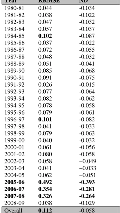
Table 2 summarizes the criteria (RRMSE and ND) computed on the basis of the 515
outputs from the two methodologies where data were replaced every 10 days for each 516
individual year (lines 1981 to 2009 in Table 2) and when the data originating from all the 517
simulations were aggregated (line ‘Overall’ in Table 2). In 90% of cases, ND values were 518
below the expected 10%, whereas RRMSE values were above the threshold in only 5 years 519
out of 29. In general, both approaches gave very close results. To a lower extend, the two 520
approaches were also equivalent for the 1984-85 and 1996-97 crop seasons, with the RRMSE 521
very close to the imposed thresholds (0.102 and 0.101, respectively). As illustrated by Figure 522
5, the 2007-08 crop season exhibited bad RRMSE and ND criteria when comparing the two 523
approaches, which was also the case for the 2005-06 and 2006-07 seasons. 524
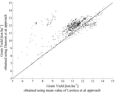
Figure 6 presents the graphical comparison of the two approaches resulting from the 525
concatenated data. The RRMSE and ND values were also computed with these data 526
(corresponding to the last ‘overall’ row in Table 2). The overall ND value revealed a slight 527
overestimation (-5.8%) using the Dumont et al. (2014b) methodology compared with the 528
Lawless and Semenov (2005) methodology. The overall RRMSE was close to the acceptable 529
value (0.112). This was due mainly to the crop seasons from 2005 to 2008; which simulations 530
are shown by the cloud of small dots in the upper left of the graph (Fig. 6) 531
The close simulations seemed qualitative enough to be able to conclude that there was 532
equivalence between the two approaches, supporting the validity of applying the Convergence 533
in Law theorem to the use of crop model. 534
3.2.2
Multiple-year analysis and prediction ability
535Finally, the statistical predictive ability of both predictive methods was compared (Fig. 536
7) using the Lawless and Semenov (2005) approach. This approach is based on determining 537
the cumulative probability function associated with the first days for which the predictions 538
would have been possible, given an error level around the final simulated value (10% in this 539
case, represented by the horizontal light dotted grey lines in Fig. 5). 540
The 2-sample Kolmogorov-Smirnov test was applied to these distributions, enabling 541
the equivalence of both distributions (p-value = 0.31) to be validated. The RMSE between the 542
two approaches was evaluated at 9 days, which is less than the rate of data replacement (10 543
days). Both approaches produced yield predictions with an equivalent lead-time. 544
4.
Discussion
545
When developing decision-support systems, crop modellers are faced with antagonist 546
decisions. On one hand, it is very important to build models and systems that can compute a 547
reasonable and reliable answer as fast as possible. At critical moments, when important 548
management decisions have to be made, farmers, who are the users of the information 549
produced, are not concerned about the time a model needs to run – they just want clear, rapid 550
answers to their questions. On the other hand, with regard to statistics, a modeller needs to 551
characterise the quality and certainty of a simulation, which makes it essential to perform 552
multi-simulations from which statistical values can be computed, to give a mean accompanied 553
by a confidence interval (e.g., 95% uncertainty limit). In addition, both practical approaches 554
need to be implemented in the spirit of the philosophy of the methodologies developed by 555
Dumont et al. (2014b) and Lawless and Semenov (2005). 556
It is worth mentioning that, although the two methodologies are generic, the results 557
presented here are site-specific. The model was parameterised and calibrated on a specific soil 558
type and for a specific crop culture. The 30-year WDB was also representative of the climatic 559
conditions of a specific area. Although generic, however, the procedure could be applied to 560
other models or model outputs. 561
4.1
Crop model behaviour analysis
562
Crop yields have finite lower and upper ranges, even under favourable climatic 563
conditions (Day, 1965), and this is especially true for crops that have a determinate growth, 564
such as wheat. Day (1965) observed, however, that determinate-growth crops skewed the 565
probability function under random weather effects, particularly when nitrogen was fertilised. 566
Our analysis confirms the observation by Day (1965) of a left-tail dissymmetry under 567
different climates. 568
It was therefore necessary to find a distribution that could account for these 569
behaviourial traits of dissymmetry and upper limitations. Our study showed that the behaviour 570
of the model could usually be correctly approximated by a log-normal distribution. This was 571
so for the stochastic climate approach and at the early stages of the within-season yield 572
prediction, i.e., provided (i) that the observed time-series were not predominant in the climatic 573
combinations or (ii) that, in the early season, observed time-series did not have a significant 574
effect on the end-season simulated yield (as illustrated in the years from 2005 to 2008). 575
With a few exceptions, the properties of the GCLT could be used to account for the 576
whole model behaviour. By extension, in this case, it is reasonable to assume that the STICS 577
model could be considered to operate as a product of functions that are themselves dependent 578
on random climatic variables. 579
4.2
Grain yield results
580
The results analysis showed a systematic and important tightening of the 95% 581
confidence curves between DOY 05/16 and 07/05. At this level, the crop had been sown about 582
200-250 days earlier. This transient period corresponds to the stages between flag-leaf 583
emergence and anthesis, the exact date being determined by the climatic conditions of the 584
relevant year. In real life, over its whole life cycle, wheat is able to compensate in order to 585
optimise its reproduction abilities. Once the number of grains is established, however, the 586
yield result depends entirely on grain filling, no matter it is driven by climatic condition 587
(linked to future data) or biomass reallocation (linked to past growing conditions). 588
Therefore, according to the simulation processes and the within-season prediction 589
methodology, as the season progresses and the hypothetical projective climatic conditions are 590
replaced by observed time-series, the number of grains is progressively fixed for each 591
simulation at a time and according to the different scenarios. Once the real weather has been 592
monitored up to the day when the number of grains has been fixed for all simulations, 593
however, the confidence boundaries become very close. From that time, as in real life, the 594
simulated yield depends entirely on grain filling and exhibits normal behaviour. During this 595
period, an observed normal distribution of grain yields would argue in favour of the 596
applicability of the CLT, instead of GCLT. Further research is needed to validate this 597
statement. 598
4.3
Predictive ability of the two approaches
599
As Dumont et al. (2014b) discussed in their work, the mean climate hypothesis is a 600
strong assumption. Seeing the climatic conditions as the mean data over the studied period is 601
equivalent to make crop growth predictions in almost non-limiting growing conditions. Under 602
such conditions, the plant will grow with little or no stress because a minimum amount of 603
water, solar radiation energy and sum of temperature are provided each day to the crop. These 604
assumptions imply that the simulated yield will correspond to the remaining yield potential of 605
the crop. This answers the question: “At a given point in the season, what could I still expect 606
at harvest if the climate tends to come back closer to the seasonal norms ?” This also implies 607
that the simulated yield could often be slightly overestimated, as confirmed by the observed 608
overall ND value (+5.8 %). 609
The conclusion that emerges from our analysis, however, is that from a strictly 610
predictive point of view the Dumont et al. (2014b) approach is equivalent to the Lawless and 611
Semenov (2005) approach (2005). In addition, during the single-year analysis the RRMSE 612
and ND criteria were close to or lower than the 10% threshold in 90% of the cases. Finally, 613
when no climatic data replacements were performed (i.e., when the yields were simulated 614
based only on pure projective stochastic climatic data or pure mean data), the difference was 615
about 7.5%. This clearly shows that the Convergence in Law theorem is applicable. 616
This fact is very important because the Dumont et al. (2014b) approach needs less 617
time (by 300-fold) to run and reach the same conclusions as the Lawless and Semenov (2005) 618
approach. The Lawless and Semenov (2005) approach is very important, however, because it 619
allows prediction uncertainty to be characterised, which is not possible with the Dumont et al. 620
(2014b) approach. When analysing climate variability or climate changes, this issue of 621
uncertainty associated with the simulations is significant. When predicting yield, however, 622
running time is a crucial factor in terms of building decision-support systems. 623
4.4
Further discussion on climatic assumption and yield distribution analysis
624
There is clear evidence that yield simulated using mean climatic data is close to the 625
yield mean obtained under stochastically generated climatic data. An overestimation has been 626
observed, though. Ongoing research (Dumont et al., 2014a ; Dumont et al., 2013) has 627
suggested that under the specific agro-pedo-climatic conditions of this case study, greater 628
skewness occurred under a fertilisation level corresponding to three applications of 60 629
kgN.ha-1 at the tillering, stem extension and flag-leaf stages, which is the fertilisation regime 630
simulated in this study. A higher degree of asymmetry leads to greater differences between the 631
mean, the median and the mode of the yield distribution. 632
This raises other discussions. First, the applicability of the Convergence in Law 633
Theorem is attractive and is compatible with the mathematical nature of crop models. As the 634
level of asymmetry is likely to decrease with other practices, the legitimacy of applying the 635
Convergence in Law Theorem should be easier to demonstrate. 636
Second, Day (1965) suggested that mode or median estimates of yield might be 637
preferred to the mean estimates, both for forecasting and prescription purposes. Our study 638
seemed to confirm this statement. The median value of yield distribution obtained using only 639
stochastic climate data (11.82 ton.ha-1) was much closer to that for yield simulated with mean 640
climate data (12.14 ton.ha-1). The analysis described in this paper should be performed using 641
the median value instead of the mean value. 642
Third, mean climate data was used as a model input. It is fairly evident that some 643
weather variables, such as temperature and solar radiation, show normal daily distributions, 644
suggesting an equivalence of the mean and median of these distributions. For some other 645
climatic data, however, daily distribution is itself asymmetric. In Belgium, rain records exhibit 646
a right-tail dissymmetry, with a high frequency of low rainfall, and low return times of 647
substantial rain. It would be interesting to assess the impact of median climatic data on the 648
corresponding simulated yield, and compare it with the yield distribution obtained 649
stochastically. 650
Finally, it is worth commenting on the generic nature of the results presented in this 651
paper. With regard to the statistical references, it could be concluded that using a model that 652
relies on similar formalisms as those of STICS models should not contradict our conclusions 653
and the GCLT would still be applicable. With regard to the crop, wheat has a determinate 654
growth and therefore it is likely that the conclusions we reached could be extended to any 655
other crop with determinate growth. Further research needs to be conducted on tuberous 656
crops, by example, such as potatoes and sugar beet, because the factors involved in tuberous 657
yield elaboration differ greatly from those in grain yield elaboration. Finally, the main 658
question to address was whether or not the Convergence in Law theorem could apply in other 659
contexts, particularly in other climatic conditions (e.g., southern Europe Mediterranean 660
weather, as in Italy or Spain) or under climatic changes. Our research suggested that if 661
climatic-induced stress remains limited in intensity or length, the GCLT would be applicable 662
to crop modelling. More work needs to be done, however, to determine the extent to which 663
this would apply given greater climatic-induced stress levels. 664
5.
Conclusion
665
In this paper, two validated methodologies for within-season wheat yield prediction, 666
one proposed by Dumont et al. (2014b) and the other by Lawless and Semenov (2005), were 667
compared. Both approaches offer the main advantage of being able to use historical data, the 668
first based on the computed mean climate and the second on using stochastically derived 669
time-series. The comparison was made using sound statistical procedures to study crop model 670
behaviour. Based on the Convergence in Law Theorem and the CLT (as well as GCLT), we 671
developed a procedure that shows how the two approaches, relying on the same weather input 672
database, could be used to make yield predictions and how close the predictions thus obtained 673
could be. 674
The generalised log-normal distribution was seen as a good way of assessing model 675
behaviour, especially when the model was run on a high number of stochastic climate inputs. 676
This is attractive because it means the model can be seen as a product of variables, which is 677
consistent with the mathematical nature of the model. It also validated the applicability of the 678
GCLT, which was a requirement in assessing the applicability of the Convergence in Law 679
Theorem. 680
Once the model behaviour had been characterised, the comparison of the yield 681
prediction ability of the two methodologies was investigated. On a year-to-year basis, the 682
analysis showed that some climatic combinations of variables could induce a bias from the 683
beginning of the season, leading to a divergence at an early stage of the predictive curves. In 684
90% of the cases, however, the differences between the two methodologies were close enough 685
to consider them as equivalent (RRMSE and ND < 10%). The inter-year analysis, which 686
related to the statistical ability of yield prediction, led to the conclusion that the two 687
methodologies had equivalent lead-time. These observations suggest that the Convergence in 688
Law theorem was validated by our case study. 689
It is important to note, however, that our work was carried out under temperate 690
Belgian weather conditions, simulating the development of a determinate wheat crop and 691
using the STICS model and the formalisms inherent in it. The procedure we designed, 692
however, is generic and should be tested on other models, under other climatic conditions and 693
with other crops before any generalisations can be made. Some generalised model behaviour 694
was highlighted, though. Crop models have been built to match reality, but contrary to real-695
life, they operate entirely according to their mathematical construction. Under fixed agro-696
pedological conditions, it should thus be possible to summarize the crop model behaviour 697
under a wide variety of climate conditions and put it in relation to a specific but relevant 698
distribution. The methodology described in this paper constituted an attempt to achieve this. 699
700
Acknowledgements
701The authors wish to thank the SPW (DGARNE - DGO-3) for its financial support for the 702
project entitled ‘Suivi en temps réel de l'environnement d'une parcelle agricole par un réseau 703
de microcapteurs en vue d’optimiser l’apport en engrais azotés’. They would also like to 704
thank the OptimiSTICS team for allowing them to re-use the Matlab running code of the 705
STICS model. The authors are very grateful to CRA-w, especially the ‘Agriculture et milieu 706
naturel’ unit, for providing them with the Ernage station climatic database. Finally, they wish 707
to thank Robert Oger for his useful help and comments on the article, as well as the two 708
anonymous reviewers for their careful review of the paper. 709