Spin-orbit angle measurements for six southern transiting planets
?
New insights into the dynamical origins of hot Jupiters
Amaury H.M.J. Triaud
1, Andrew Collier Cameron
2, Didier Queloz
1, David R. Anderson
3, Micha¨el Gillon
4, Leslie
Hebb
5, Coel Hellier
3, Benoˆıt Loeillet
6, Pierre F. L. Maxted
3, Michel Mayor
1, Francesco Pepe
1, Don Pollacco
7, Damien
S´egransan
1, Barry Smalley
3, St´ephane Udry
1, Richard G. West
8, and Peter J. Wheatley
91 Observatoire Astronomique de l’Universit´e de Gen`eve, Chemin des Maillettes 51, CH-1290 Sauverny, Switzerland 2 School of Physics & Astronomy, University of St Andrews, North Haugh, St Andrews KY16 9SS, Fife, Scotland, UK 3 Astrophysics Group, Keele University, Staffordshire ST55BG, UK
4 Institut d’Astrophysique et de G´eophysique, Universit´e de Li`ege, All´ee du 6 Aoˆut, 17, Bat. B5C, Li`ege 1, Belgium 5 Department of Physics and Astronomy, Vanderbilt University, Nashville, TN37235, USA
6 Laboratoire d’Astrophysique de Marseille, BP 8, 13376 Marseille Cedex 12, France
7 Astrophysics Research Centre, School of Mathematics & Physics, Queens University, University Road, Belfast BT71NN, UK 8 Department of Physics and Astronomy, University of Leicester, Leicester LE17RH, UK
9 Department of Physics, University of Warwick, Coventry CV4 7AL, UK Received date/ accepted date
ABSTRACT
Context.There are competing scenarii for planetary systems formation and evolution trying to explain how hot Jupiters came to be
so close to their parent star. Most planetary parameters evolve with time, making distinction between models hard to do. It is thought the obliquity of an orbit with respect to the stellar rotation is more stable than other parameters such as eccentricity. Most planets, to date, appear aligned with the stellar rotation axis; the few misaligned planets so far detected are massive ( > 2 MJ).
Aims.Our goal is to measure the degree of alignment between planetary orbits and stellar spin axes, to detect potential correlation
with eccentricity or other planetary parameters and to measure long term radial velocity variability indicating the presence of other bodies in the system.
Methods.For transiting planets, the Rossiter-McLaughlin effect allows the measurement of the sky-projected angle β between the
stellar rotation axis and a planet’s orbital axis. Using the HARPS spectrograph, we observed the Rossiter-McLaughlin effect for six transiting hot Jupiters found by the WASP consortium. We combine these with long term radial velocity measurements obtained with CORALIE. We used a combined analysis of photometry and radial velocities, fitting models with a Markov Chain Monte Carlo. After obtaining β we attempt to statistically determine the distribution of the real spin-orbit angle ψ.
Results.We found that three of our targets have β above 90◦
: WASP-2b: β= 153◦+11
−15, WASP-15b: β= 139.6 ◦+5.2
−4.3and WASP-17b: β = 148.5◦+5.1
−4.2; the other three (WASP-4b, WASP-5b and WASP-18b) have angles compatible with 0 ◦
. There is no dependence between the misaligned angle and planet mass nor with any other planetary parameter. All orbits are close to circular, with only one firm detection of eccentricity on WASP-18b with e = 0.00848+0.00085−0.00095. No long term radial acceleration was detected for any of the targets. Combining all previous 20 measurements of β and our six and transforming them into a distribution of ψ we find that between about 45 and 85 % of hot Jupiters have ψ > 30◦
.
Conclusions.Most hot Jupiters are misaligned, with a large variety of spin-orbit angles. We find observations and predictions using
the Kozai mechanism match well. If these observational facts are confirmed in the future, we may then conclude that most hot Jupiters are formed from a dynamical and tidal origin without the necessity to use type I or II migration. At present, standard disc migration cannot explain the observations without invoking at least another additional process.
Key words.binaries: eclipsing – planetary systems – stars: individual: WASP-2, WASP-4, WASP-5, WASP-15, WASP-17, WASP-18
– techniques: spectroscopic
1. Introduction
The formation of close-in gas giant planets, the so-called hot Jupiters, has been in debate since the discovery of the first of them, 51 Peg b, by Mayor & Queloz (1995). The repeated ob-servations of these planets in radial velocity and the discovery
Send offprint requests to: Amaury.Triaud@unige.ch
? using observations with the high resolution ´echelle spectrograph HARPS mounted on the ESO 3.6 m (under proposals 072.C-0488, 082.C-0040 & 283.C-5017), and with the high resolution ´echelle spec-trograph CORALIE on the 1.2 m Euler Swiss Telescope, both installed at the ESO La Silla Observatory in Chile. The data is made publicly available at CDS - Strasbourg
with HD 209548b (Charbonneau et al. 2000; Henry et al. 2000) that some of them transit has produced a large diversity in plane-tary parameters, such as separation, mass, radius (hence density) and eccentricity. Although more than 440 extrasolar planets have been discovered, of which more than 70 are known to transit, we are still increasing the range of parameters that planets occupy; diversity keeps growing.
While it is generally accepted that close-orbiting gas-giant planets do not form in-situ, their previous and subsequent evolu-tion is still mysterious. Several processes can affect the planet’s eccentricity and semi-major axis. Inward migration via angular momentum exchange with a gas disc, first proposed in Lin et al.
(1996) from work by Goldreich & Tremaine (1980), is a natural and widely-accepted explanation for the existence of these hot Jupiters.
Migration alone does not explain the observed distribu-tions in eccentricity and semi-major axis that planets occupy. Alternative mechanisms have therefore been proposed such as the Kozai mechanism (Kozai 1962; Eggleton & Kiseleva-Eggleton 2001; Wu & Murray 2003) and planet scattering (Rasio & Ford 1996). These mechanisms can also cause a planet to migrate inwards, and may therefore have a role to play in the formation and evolution of hot Jupiters. These different mod-els each predict a distribution in semi-major axis and eccentric-ity. Discriminating between various models is done by matching the distributions they produce to observations. Unfortunately this process does not take into account the evolution with time of the distributions and is made hard by the probable combination of a variety of effects.
On transiting planets, a parameter can be measured which might prove a better marker of the past history of planets: β, the projection on the sky of the angle between the star’s rotation axis and the planet’s orbital axis. It is believed that the obliquity (the real spin-orbit angle ψ) of an orbit evolves only slowly and is not as much affected by the proximity of the star as the eccentric-ity (Hut 1981; Winn et al. 2005; Barker & Ogilvie 2009). Disc migration is expected to leave planets orbiting close to the stel-lar equatorial plane. Kozai cycles and planet scattering should excite the obliquity of the planet and should provide us with a planet population on misaligned orbits with respect to their star’s rotation.
As a planet transits a rotating star, it will cause an overall red-shifting of the spectrum if it covers the blue-shifted half of the star and vice-versa on the other side. This is called the Rossiter-McLaughin effect (Rossiter 1924; McLaughlin 1924). It was first observed for a planet by Queloz et al. (2000). Several papers model this effect: Ohta et al. (2005); Gim´enez (2006); Gaudi & Winn (2007).
Among the 70 or so known transiting planets discovered since 2000 by the huge effort sustained by ground-based transit-ing planet searches, the Rossiter-McLaughlin (RM) effects have been measured for 20, starting with observations on HD 209458 by Queloz et al. (2000). This method has proven itself reliable at giving precise and accurate measurement of the projected spin-orbit angle with its best determination done for HD 189733b (Triaud et al. 2009). Basing their analysis on measurements of β in 11 systems, 10 of which are coplanar or nearly so, Fabrycky & Winn (2009) concluded that the angle distribution is likely to be bimodal with a coplanar population and an isotropically-misaligned population. At that time, the spin-orbit misalignment of XO-3b (H´ebrard et al. 2008) comprised the only evidence of the isotropic population. Since then, the misalignment of XO-3b has been confirmed by Winn et al. (2009c), and significant misalignments have been found for HD 80606b (Moutou et al. 2009) and WASP-14b (Johnson et al. 2009). Moreover, retro-grade orbital motion has been identified in HAT-P-7b (Winn et al. 2009b; Narita et al. 2009). Other systems show indica-tions of misalignment but need confirmation. One such object is WASP-17b (Anderson et al. 2010) which is one of the subjects of the present paper.
The Wide Angle Search for Planets (WASP) project aims at finding transiting gas giants (Pollacco et al. 2006). Observing the northern and southern hemispheres with sixteen 11 cm refractive telescopes, the WASP consortium has published more than 20
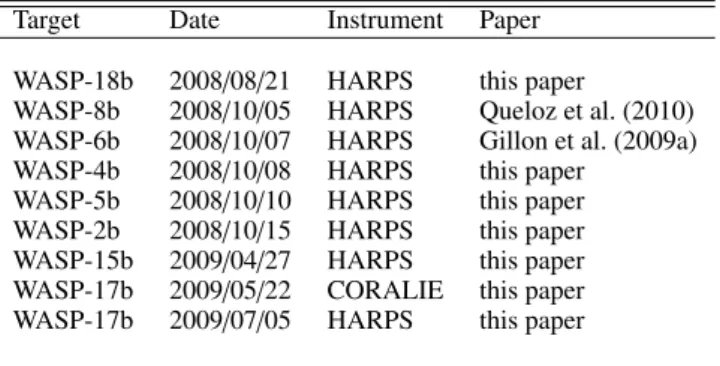
Table 1. List of Observations. The date indicates when the first point of the Rossiter-McLaughlin sequence was taken.
Target Date Instrument Paper WASP-18b 2008/08/21 HARPS this paper
WASP-8b 2008/10/05 HARPS Queloz et al. (2010) WASP-6b 2008/10/07 HARPS Gillon et al. (2009a) WASP-4b 2008/10/08 HARPS this paper
WASP-5b 2008/10/10 HARPS this paper WASP-2b 2008/10/15 HARPS this paper WASP-15b 2009/04/27 HARPS this paper WASP-17b 2009/05/22 CORALIE this paper WASP-17b 2009/07/05 HARPS this paper
transiting planets in a large range of period, mass and radius, around stars with apparent magnitudes between 9 and 13. The planet candidates observable from the South are confirmed by a large radial-velocity follow-up using the CORALIE high reso-lution ´echelle spectrograph, mounted on the 1.2 m Euler Swiss Telescope, at La Silla, Chile. As part of our efforts to understand the planets that have been discovered, we have initiated a sys-tematic program to measure the Rossiter-McLaughlin effect in the planets discovered by the WASP survey, in order to measure their projected spin-orbit misalignment angles β.
In this paper we report the measurement of β in six south-ern transiting planets from the WASP survey, and analyse their long term radial velocity behaviour. In sections 2 and 3 we de-scribe the observations and the methods employed to extract and analyse the data. In section 4 we report in detail on the Rossiter-McLaughlin effects observed during transits of the six systems observed. In sections 5 and 6 we discuss the correlations and trends that emerge from the study and their implications for plan-etary migration models.
2. The Observations
In order to determine precisely and accurately the angle β, we need to obtain radial velocities during planetary transits at a high cadence and high precision. We therefore observed with the high resolution ´echelle spectrograph HARPS, mounted at the La Silla 3.6 m ESO telescope. The magnitude range within which planets are found by the SuperWASP instruments allows us to observe each object in adequate conditions. For the main survey pro-posal 082.C-0040, we selected as targets the entire population of transiting planets known at the time of proposal submission to be observable from La Silla during Period 82, i.e. WASP-2b, 4b, 5b, 6b, 8b and 15b. The results for WASP-6b are presented separately by Gillon et al. (2009a) and for WASP-8b by Queloz et al. (2010). Two targets were added in separate proposals. A transit of WASP-18b was observed during GTO time (072C-0488) of the HARPS consortium allocated to this planet because of its short and eccentric orbit. During the long-term spectro-scopic follow-up of WASP-17b undertaken for the discovery pa-per (Anderson et al. 2010), three CORALIE measurements fell during transit showing a probably retrograde orbit. Observations of the Rossiter-McLaughlin with CORALIE confirmed the con-clusions of Anderson et al. (2010), and a follow-up DDT pro-posal (283.C-5017) was awarded time on HARPS.
The strategy of observations was to take two high precision HARPS points the night before transit and the night after transit. The radial-velocity curve was sampled densely throughout the
are used as priors in the analysis. ξtis the microturbulence. Vmacrois the macrotrubulence.
Parameters units WASP-2 (a,b) WASP-4 (c) WASP-5 (c) WASP-15 (d) WASP-17 (a,e) WASP-18 (f)
Spectral Type K1 G8 G5 F7 F4 F6 Teff K 5150 ± 80 5500 ± 100 5700 ± 100 6300 ± 100 6650 ± 80 6400 ± 100 B − V mag 0.86 ± 0.05 0.73 ± 0.05 0.66 ± 0.05 0.48 ± 0.05 0.38 ± 0.05 0.45 ± 0.05 log g dex 4.40 ± 0.15 4.5 ± 0.2 4.5 ± 0.2 4.35 ± 0.15 4.45 ± 0.15 4.4 ± 0.15 [Fe/H] dex −0.08 ± 0.08 −0.03 ± 0.09 +0.09 ± 0.09 −0.17 ± 0.11 −0.19 ± 0.09 0.00 ± 0.09 log R0 HK dex −4.84 ± 0.10 −4.50 ± 0.06 −4.72 ± 0.07 −4.86 ± 0.05 - −4.85 ± 0.02 ξt km s−1 0.9 ± 0.1 1.1 ± 0.2 1.2 ± 0.2 1.4 ± 0.1 1.7 ± 0.1 1.6 ± 0.1 Vmacro km s−1 1.6 ± 0.3 2.0 ± 0.3 2.0 ± 0.3 4.8 ± 0.3 6.2 ± 0.3 4.8 ± 0.3 vsin I km s−1 1.6 ± 0.7 2.0 ± 1.0 3.5 ± 1.0 4.0 ± 2.0 9.8 ± 0.5 11.0 ± 1.5 M? M 0.84 ± 0.11 0.93 ± 0.05 1.00 ± 0.06 1.18 ± 0.12 1.2 ± 0.12 1.24 ± 0.04
Note 1. references: (a) this paper, (b) Cameron et al. (2007), (c) Gillon et al. (2009c), (d) West et al. (2009), (e) Anderson et al. (2010), (f) Hellier et al. (2009)
transit, beginning 90 minutes before ingress and ending 90 min-utes after egress. The data taken before ingress and after egress allow any activity-related offset in the effective velocity of the system’s centre of mass to be determined for the night of obser-vation. In addition, radial velocity data from the high resolution ´echelle spectrograph CORALIE mounted on the Swiss 1.2 m EulerTelescope, also at La Silla was acquired to help search for a long term variability in the the periodic radial velocity signal.
All our HARPS observations have been conducted in the OBJO mode, without simultaneous Thorium-Argon spectrum. The velocities are estimated by a Thorium-Argon calibration at the start of the night. HARPS is stable within 1 m s−1across a
night. This is lower than our individual error bars and leads to no contamination of the Th-Ar lamp onto the stellar spectrum easing spectral analysis.
3. The Data Analysis
3.1. Radial-velocity extraction
The spectroscopic data were reduced using the online Data Reduction Software (DRS) which comes with HARPS. The ra-dial velocity information was obtained by removing the instru-mental blaze function and cross-correlating each spectrum with one of two masks. This correlation is compared with the Th-Ar spectrum acting as a reference; see Baranne et al. (1996), Pepe et al. (2002) & Mayor et al. (2003) for details. Recently the DRS was shown to achieve remarkable precision (Mayor et al. 2009) thanks to a revision of the reference lines for Thorium and Argon by Lovis & Pepe (2007). Stars with spectral type earlier than G9 were reduced using the G2 mask, while those of K0 or later were cross-correlated with the K5 mask. A similar software package is used for CORALIE data. A resolving power R = 110 000 for HARPS yields a cross-correlation function (CCF) binned in 0.25 km s−1increments, while for CORALIE, with a lower
res-olution of 50 000, we used 0.5 km s−1. The CCF window was adapted to be three times the size of the full width at half maxi-mum (FWHM) of the CCF.
All our past and current CORALIE data on the stars pre-sented here were reprocessed after removal of the instrumen-tal blaze response, thereby changing slightly some radial
veloc-ity values compared to those already published in the literature. Correcting this blaze is important for extracting the correct RVs for the RM effect. The uncorrected blaze created a slight sys-tematic asymmetry in the CCF that was translated into a bias in radial velocities.
1 σ error bars on individual data points were estimated from photon noise alone. HARPS is stable long term within 1 m s−1
and CORALIE at less than 5 m s−1. These are smaller than our individual error bars and thus have not been taken into account.
3.2. Spectral analysis
Spectral analysis is needed to determine the stellar atmospheric parameters from which limb darkening coefficients can be in-ferred. We carried out new analyses for two of the target stars, WASP-2 and WASP-17, whose previously-published spectro-scopic parameters were of low precision. For our other targets, the atmospheric parameters were taken from the literature, no-tably the stellar spectroscopic rotation broadening v sin I1.
The individual HARPS spectra can be co-added to form an overall spectrum above S/N ∼ 1 : 100, suitable for photospheric analysis which was performed using the uclsyn spectral synthe-sis package (Smith 1992; Smalley et al. 2001) and atlas9 mod-els without convective overshooting (Castelli et al. 1997) and the same method as described in many discovery papers published by the WASP consortium (eg: Wilson et al. (2008)).
The stellar rotational v sin I is determined by fitting the pro-files of several unblended Fe i lines. The instrumental FWHM was determined to be 0.065Å from the telluric lines around 6300Å.
For WASP-2, a value for macroturbulence (vmac) of 1.6 ±
0.3 km s−1 was adopted (Gray 2008). A best fitting value of
vsin I = 1.6 ± 0.7 km s−1was obtained. On WASP-17, a value for macroturbulence (vmac) of 6.2 ± 0.3 km s−1was used (Gray
2008). The analysis gives a best fitting value of v sin I= 9.8 ± 1 throughout this paper we use the symbol I to denote the inclination of the stellar rotation axis to the line of sight, while i represents the inclination of the planet’s orbital angular momentum vector to the line of sight
0.5 km s−1. The error on vmacis taken from the scatter around fit
to Gray (2008) and is propagated to the v sin I .
B−Vwere estimated from the effective temperature and used in the calculations of the log R0
HK(Noyes et al. 1984; Santos et al.
2000; Boisse et al. 2009). Errors refer to the photon noise: they do not include systematic effects likely to arise and affect low values of log R0HK due to the low signal to noise in the blue or-ders. WASP-17 does not have a value since this stellar activity indicator is only calibrated for B − V ∈ [0.44, 1.20].
All stellar parameters, used as well as derived, are presented in Table 2.
3.3. Model fitting
The extracted radial velocity data was fitted simultaneously with the transit photometry available at the time of analysis. Three models are adjusted to the data: a Keplerian radial velocity or-bit (Hilditch 2001), a photometric planetary transit (Mandel & Agol 2002), and a spectroscopic transit, also known as Rossiter-McLaughlin effect (Gim´enez 2006). This combined approach is very useful for taking into account all of the possible contribu-tions to the uncertainties due to correlacontribu-tions among all relevant parameters. A single set of parameters describes both the pho-tometry and the radial velocities. We use a Markov Chain Monte Carlo (MCMC) approach to optimize the models and estimate the uncertainties of the fitted parameters. The fit of the model to the data is quantified using the χ2statistic.
The code is described in detail by Triaud et al. (2009), has been used several times (eg: Gillon et al. (2009a)) and is similar to the code described in Cameron et al. (2007).
We fitted up to 10 parameters, namely the depth of the pri-mary transit D, the radial velocity (RV) semi-amplitude K, the impact parameter b, the transit width W, the period P, the epoch of mid-transit T0, e cos ω, e sin ω, V sin I cos β, and V sin I sin β.
Here e is the eccentricity and ω the angle between the line of sight and the periastron, V sin I is the sky-projected rotation ve-locity of the star2while β is the sky-projected angle between the
stellar rotation axis (Hosokawa 1953; Gim´enez 2006) and the planet’s orbital axis3.
These parameters have been chosen to reduce correlations between then. The use of uncorrelated parameters allows to explore parameter space more efficiently since the correlation length between jumps is smaller. Eccentricity and periastron an-gle were paired as were V sin I and β. This breaks a correlation between them (the reader is invited to compare Figs. 2d & 3 for a clear illustration for choosing certain jump parameters as op-posed to others). This way we also explore solutions around zero more easily: e cos ω and e sin ω move in the ]-1,1[ range while e could only be floating in ]0,1[. For exploring particular solutions such as a circular orbit, parameters can be fixed to certain values. We caution that, as noted by Ford (2006) that the choice of e cos ω and e sin ω as jump variables implicitly imposes a prior that is proportional to e. This approach thus has a ten-dency to yield a higher eccentricity than would be obtained with a uniform prior, in cases when e is poorly-constrained by the data. A similar argument applies to the use of V sin I cos β and 2 we make a distinction between v sin I and V sin I: v sin I is the value extracted from the spectral analysis, the stellar spectroscopic rotation broadening, while V sin I denotes the result of a Rossiter-McLaughlin effect fit. Both can at times be different. Each, although caused by the same effect, is independently measured making the distinction worth-while.
3 β = −λ, another notation used in the literature for the same angle.
Vsin I sin β as jump variables, in cases where the impact param-eter is low and there is a strong degeneracy between V sin I and β in modelling the Rossiter-McLaughlin effect. In such cases, however, the tendency to overestimate V sin I from the Rossiter-McLaughlin effect can effectively be curbed by imposing an in-dependent, spectroscopically-determined v sin I prior on V sin I, as we have done here.
In addition to the physical free floating parameters, we need to use one γ velocity for each RV set and one normalisation factor for each lightcurve as adjustment parameters. These are found by using optimal averaging and optimal scaling. γ veloc-ities represent the mean radial velocity of the star in space with respect to the barycentre of the Solar System. Since our analysis had many datasets, the results for these adjustment parameters have been omitted, not adding anything to the discussion.
During these initial analyses we also fitted an additional ac-celeration in the form of an RV drift ˙γ but on no occasion was it significantly different from zero. We therefore assumed there was no drift for any of our objects. We will give upper limits for each star in the following sections.
The MCMC algorithm perturbs the fitting parameters at each step i with a simple formula:
Pi, j= Pi−1, j+ f σPjG(0, 1) (1)
where Pjis a free parameter, G is a Gaussian random number of
unit standard deviation and zero mean (meaning a Gaussian prior on each parameter), while σ is the step size for each parameter. A factor f is used to control the chain and ensures that 25 % of steps are being accepted via a Metropolis-Hastings algorithm, as recommended in Tegmark et al. (2004) to give an optimal exploration of parameter space.
The step size is adapted by doing several initial analyses. They are adjusted to produce as small a correlation length as possible. Once the value is chosen, it remains fixed. Only f fluc-tuates.
A burn-in phase of 50 000 accepted steps is used to make the chain converge. This is detected when the correlation length of each parameter is small and that the average χ2does not
im-prove anymore (Tegmark et al. 2004). Then starts the real chain, of 500 000 accepted steps, from which results will be extracted. This number of steps is used as a compromise between computa-tion time and exploracomputa-tion. Statistical tests, notably by comparing χ2are used to estimate the significance of the results.
Bayesian penalties acting as prior probability distribution can be added to χ2 to account for any prior information that
we might have on any fitted or derived parameter. Stellar mass M?can notably be inserted via a prior in the MCMC in order to propagate its error bars on the planet’s mass. We also inserted the vsin I found by spectral analysis as priors in some of our fits to control how much the fit was dependent on them and the result-ing value of V sin I and whether this influenced the fitted value of β. Because of the random nature of an MCMC, sometimes a step with an impact parameter close to zero is taken. This can cause V sin I to wander to unphysical values because of the de-generacy between V sin I and β at low impact parameters. This is controlled by imposing a prior. The prior values are in Table 2.
We use a quadratic limb-darkening law with fixed values for the two limb darkening coefficients appropriate to the stel-lar effective temperature. They were extracted for the photom-etry from tables published in Claret (2000). For the radial ve-locity (the Rossiter-McLaughlin effect is also dependent on limb darkening) we use values for the V band. Triaud et al. (2009) showed that HARPS is centred on the V band. The coefficients
−60 −40 −20 0 20 40 60 −0.04 −0.02 0.00 0.02 0.04 −20 0 20 Phase Radial Velocities (m.s − 1) Residuals (m.s − 1) . . . . −100 0 100 −0.4 −0.2 0.0 0.2 0.4 −50 0 50 Phase Radial Velocities (m.s − 1) Residuals (m.s − 1) . .
a)
b)
c)
d)
Fig. 1. Fit results for WASP-2b. a) Overall Doppler shift reflex motion of the star due to the planet and residuals. b) Zoom on the Rossiter-McLaughlin effect and residuals. Black inverted triangles are SOPHIE data, black triangles represent CORALIE points, red dots show the HARPS data. The best fit model is also pictured as a plain blue line. In addition to our best model found with V sin I = 0.99 km s−1we also present models with no RM effect plotted as a dotted blue line, RM effect with β = 0 and Vsin I= 0.9 km s−1drawn with a dashed-dotted blue line and RM effect with β = 0 and V sin I = v sin I = 1.6 km s−1pictured with
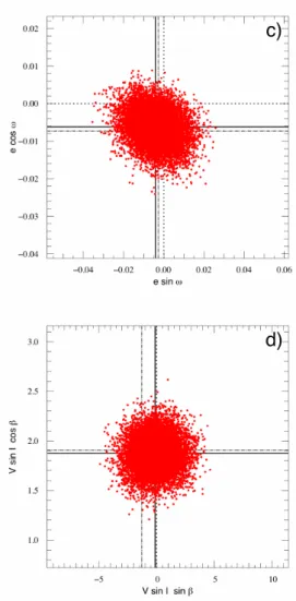
a dashed-double dotted blue line. In the residuals, the open symbols represent in the values with the size of the circle decreasing with the likelyhood of the model. c) Posterior probability distribution issued from the MCMC showing the distribution of points between e cos ω and e sin ω. d) Posterior probability distribution issued from the MCMC showing the distribution of points between Vsin I cos β and V sin I sin β. The black disc shows where the distribution would be centred only changing to β = 0. The dotted line shows where zero is. The straight lines represent the median of the distribution, the dashed lines plot the position of the average values, the dash-dotted lines indicate the values with the lowest χ2(some lines can overlap). The size of boxes c) and d) represents 7 times the 1 σ distance on either side of the median.
were chosen for atmospheric parameters close to those presented in Table 2.
3.4. Extracting the results
For each star, we performed four analyses, each using a MCMC chain with 500 000 accepted steps:
– 1. a prior is imposed on V sin I, eccentricity is fixed to zero; – 2. no prior on V sin I, eccentricity is fixed to zero;
– 3. a prior is imposed on V sin I, eccentricity is let free; – 4. no prior on V sin I, eccentricity is let free.
This is to assess the sensitivity of the model parameters to a small but uncertain orbital eccentricity and to the v sin I value
found by spectral analysis which, as demonstrated in Triaud et al. (2009), can seriously affect the fitting of the Rossiter-McLaughlin effect. The comparative tables holding the results of these various fits are available in the appendices to support the conclusions we reach while allowing readers to form their own opinion. In addition, we also conducted control chains fixing the parameters controlled by the photometry in order to check whether this was a limiting source of errors in the determina-tion of our most important parameter: β. The results from these chains are in the appendices as well. Although different in their starting hypotheses all the chains are also useful at checking their respective convergence. Our final results are presented in Table 3.
The best solution is found in the best of the four fits by com-paring χ2and using Ockham’s principle of minimising the
num-ber of parameters for similar results: for fits with similar χ2reduced we usually choose a circular solution with no prior on V sin I. Results are extracted from the best fit by taking the median of the posterior probability distribution for each parameter, deter-mined from the Markov chain. Errors bars are estimated from looking at the extremes of the distribution comprising the 68.3 % confidence region of the accepted steps. The best solution is not taken from the lowest χ2as it is dependent on the sampling and chance encounter of a - small - local minimum. Scatter plots will be presented with the positions of the best χ2, the average and the median for illustration.
In the following section and in tables, several statistical val-ues are used: χ2 is the value found for all the data, while χ2
RV
gives the value of χ2solely for the radial velocities. The reduced
χ2 for the radial velocities, denoted by χ2
reduced, is used to
esti-mate how well a model fits the data and to compare various fits and their respective significance. In addition we will also use the residuals, denoted as O − C. These estimates are only for radial velocities. The results from photometry are not mentioned since they are not new. They are only here to constrain the shape of the Rossiter-McLaughlin effect.
When giving bounds, for eccentricity and long term radial velocity drift, we quote the 95% confidence interval for exclu-sion.
4. The Survey Results
4.1. WASP-2b
A sequence of 26 RV measurements was taken on WASP-2 us-ing HARPS on 2008 October 15, with additional observations made outside transit as given in the journal of observations pre-sented in the appendices. The cadence during transit was close to a point every 430s. The average photon noise error of that sequence is 5.7 m s−1. We made additional observations with CORALIE to refine the orbital solution obtained by Cameron et al. (2007) using the SOPHIE instrument on the 1.93 m tele-scope at Observatoire de Haute-Provence, and to look for long-term variability of the orbit. 20 measurements were taken with a mean precision of 13.9 m s−1over close to 11 months between 2008 October 25 and 2009 September 23. All the RV data is available in the appendices along with exposure times.
To establish the photometric ephemeris and the transit geom-etry, we fitted the photometric datasets of Cameron et al. (2007) (3 seasons by SuperWASP in the unfiltered WASP bandpass), Charbonneau et al. (2007) (a z band Keplercam lightcurve) and Hrudkov´a et al. (2009) (a William Herschel Telescope AG2 R band transit curve).
WASP-2b’s data were fitted with up to 10 free parameters plus 8 independent adjustment parameters: three γ velocities for the three RV data sets and five normalisation factors for photom-etry. This sums up to 58 RV measurements and 8951 photometric observations.
χ2
reduceddoes not improve significantly between circular and
eccentric models. We therefore impose a circular solution. The presence of a prior on V sin I does not affect the results. We find Vsin I = 0.99+0.27−0.32 km s−1 in accordance with the v sin I value
found in section 3.2. The fit delivers β = 153◦+11
−15. The overall
root-mean-square (RMS) scatter of the spectroscopic residuals about the fitted model is 11.73 m s−1. During the HARPS transit
sequence these residuals are at 6.71 m s−1.
Fig. 3 shows the resulting distribution as V sin I vs. β. We detect V sin I significantly above zero with confidence interval showing that 99.73% (3 σ) of the posterior probability function has V sin I > 0.2 km s−1while β > 77.26◦. We have computed 6
additional chains in order to test the strength of our conclusions. Table A.1 shows the comparison between the various fits; we invite the reader to refer to it as only important results are given in the text.
In all cases, eccentricity is not detected being below a 3 σ significance from circular which is likely affected from the poor coverage of the phase by the HARPS points. Circular solutions are therefore adopted. We fix the eccentricity’s upper limit to e< 0.070. In addition no significant long term drift was detected in the spectroscopy: | ˙γ| < 36 m s−1yr−1.
Using the spectroscopically-determined v sin I value of 1.6 km s−1and forcing β to zero, χ2
reducedchanges from 2.14±0.27
to 3.49 ± 0.39, clearly degrading the solution. We are in fact 7.6 σ away from the best-fitting solution, therefore excluding an aligned system with this large a V sin I. This is also excluded by comparison to a fit with a flat RM effect at the 6.7 σ. Similarly, a fit with an imposed V sin I = 0.9 km s−1 and aligned orbit is found 5.6 σ from our solution. On Fig 1b, we have plotted the various models tested and their residuals so as to give a visual demonstration of the degradation for each of the alternative so-lutions.
4.2. WASP-4b
We obtained a RM sequence of WASP-4b with HARPS on 2008 October 8; other, out of transit, measurements are reported in the journal of observations given in the appendices. The RM sequence comprises 30 data points, 13 of which are in transit, taken at a cadence of 630 s−1with a mean precision of 6.4 m s−1. The spectrograph CORALIE continued monitoring WASP-4 and we add ten radial velocity measurements to the ones published in Wilson et al. (2008). These new data were observed around the time of the HARPS observations, about a year after spectro-scopic follow-up started.
In photometry we gathered 2 timeseries in the WASP band-pass from Wilson et al. (2008) and an R band C2 Euler transit plus a VLT/FORS2 z band lightcurve obtained from Gillon et al. (2009c) to establish the transit shape and timing.
The WASP-4b data were fitted with up to 10 free parameters to which 6 adjustment parameters were added: two γ velocities for RVs and four normalisation factors for the photometry. In to-tal, this represents 56 radial velocity points and 9989 photomet-ric measurements. Gillon et al. (2009c) let combinations of limb darkening coefficients free to fit the high precision VLT curve. We used and fixed our coefficients on their values.
Because the impact parameter is small, a degeneracy be-tween β and V sin I appeared, as expected (see Figs. 2d & 3). The values on stellar rotation for our unconstrained fits reach unphysical values as high as V sin I = 150 km s−1. We imposed
a prior on the stellar rotation to restrict it to values consistent with the spectroscopic analysis.
The reduced χ2 is the same within error bars whether ec-centricity if fitted or fixed to zero. Therefore the current best solution, by minimising the number of parameters, is a circular orbit.
The eccentricity is constrained to e < 0.0182. Thanks to the long time series in spectroscopy we also investigated the pres-ence of a long term radial velocity trend. Nothing was signifi-cantly detected: | ˙γ| < 30 m s−1yr−1.
−100 −50 0 50 100 −0.10 −0.05 0.00 0.05 0.10 −60 −40 −20 0 20 40 60 Phase Radial Velocities (m.s − 1) Residuals (m.s − 1) . . . . −200 −100 0 100 200 −0.4 −0.2 0.0 0.2 0.4 −50 0 50 Phase Radial Velocities (m.s − 1) Residuals (m.s − 1) . .
a)
b)
c)
d)
Fig. 2. Fit results for WASP-4b. Nota Bene: Legend similar to the legend in Fig.1.
Because of the small impact parameter the spin-orbit angle is poorly constrained with β = −4◦+43−34, even when a prior is imposed on V sin I. The high S/N of the Rossiter-McLaughlin effect allows us to exclude a projected retrograde orbit.
4.3. WASP-5b
Using HARPS, we took a series of 28 exposures on WASP-5 at a cadence of roughly 630s with a mean photon noise of 5.5 m s−1 on 2008 October 16. Other measurements were obtained at dates before and after this transit. Five additional CORALIE spectra were acquired the month before the HARPS observations. They were taken about a year after the data published in Anderson et al. (2008). All spectroscopic data is available from the appen-dices.
To help determine transit parameters, published photometry was assembled and comprises three seasons of WASP data, two C2 Eulerlightcurves in R band, and one FTS i0band lightcurve (Anderson et al. 2008).
WASP-5b’s 49 RV measurements and 14 754 photometric points were fitted with up to 10 free parameters to which 8 ad-justment parameters had to be added: two γ velocities and six normalisation factors.
The imposition of a prior on V sin I prior makes little im-pact on the final results (see appendices) and their 1σ error bars but prevents V sin I to go to unphysical values when, through the random process of the MCMC, the impact parameter b gets very close to zero on a few occasions. We choose the solution using a prior. The priorless solution gives a V sin I fully consis-tent with v sin I thereby obtaining an independent measurement of the projected stellar equatorial rotation speed. Allowing ec-centricity to float did not produce a significantly better fit. It has a 99.6 % chance of being different from zero: at 2.9 σ. Thus, minimising the number of parameters for a similar fit, we chose the solution with a circular orbit and simply place an upper limit on the eccentricity: e < 0.0351. No long term RV trend appears at this date: | ˙γ| < 47 m s−1yr−1.
Parameters extracted are similar to those that were pub-lished in Gillon et al. (2009c) & Anderson et al. (2008) and with Southworth et al. (2009) using a independent dataset. The projection of the spin-orbit angle is found to be: β = −12.1◦+10.0
−8.0 and we obtain an independent measurement of
Vsin I = 3.24+0.34−0.35km s−1 fully compatible with the spectral
value that was used as a prior in other fits. Results are presented in Table 3.
The χ2
reducedfor spectroscopy (see Table A.1) is quite large, at
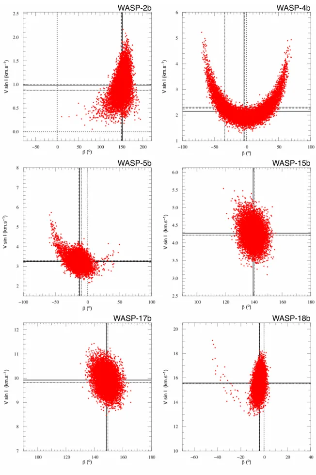
WASP-2b
WASP-4b
WASP-5b
WASP-15b
WASP-18b
WASP-17b
Fig. 3. Posterior probability distribution issued from the MCMC showing the resulting distributions of points between V sin I and β for our six WASP targets. These distributions are issued from the chains that gave our preferred solutions as explained in the text. The dotted lines show where zeros are, the straight lines represent the medians of the distributions, the dashed lines plot the positions of the average values, the dash-dotted lines indicate the values with the lowest χ2(some lines can overlap). The scale of
the boxes was adapted to include the whole distibutions. 8
T able 3. Fitted and ph ysical parameters found after fitting photometric and spectroscopic data of W ASP-4b with a prior on V sin I. The v alue from eccentricity w as found using information from other fits as explained in the te xt. P arameters unit s W ASP-2b W ASP-4b W ASP-5b W ASP-15b W ASP-17b W ASP-18b fitted par ameter s D 0 .01802 + 0 .00027 − 0 .00025 0 .023334 + 0 .000044 − 0 .000072 0 .01223 + 0 .00040 − 0 .00014 0 .00969 + 0 .00013 − 0 .00011 0 .01672 + 0 .00020 − 0 .00016 0 .00916 + 0 .00020 − 0 .00012 K m s − 1 153 .6 + 3 .0 − 3 .1 242 .1 + 2 .8 − 3 .1 268 .7 + 1 .8 − 1 .9 64 .6 + 1 .20 − 1 .25 52 .7 + 3 .0 − 2 .8 1816 .7 + 1 .9 − 1 .9 b R? 0 .737 + 0 .012 − 0 .013 0 .051 + 0 .023 − 0 .049 0 .37 + 0 .11 − 0 .06 0 .525 + 0 .037 − 0 .028 0 .400 + 0 .043 − 0 .040 0 .527 + 0 .052 − 0 .046 W days 0 .07372 + 0 .00065 − 0 .00068 0 .08868 + 0 .00008 − 0 .000014 0 .0988 + 0 .0013 − 0 .0005 0 .1547 + 0 .0012 − 0 .0009 0 .1843 + 0 .0013 − 0 .0010 0 .09089 + 0 .00080 − 0 .00061 P days 2 .1522254 + 0 .0000015 − 0 .0000014 1 .3382299 + 0 .0000023 − 0 .0000021 1 .6284229 + 0 .0000043 − 0 .0000039 3 .752100 + 0 .000009 − 0 .000011 3 .7354330 + 0 .0000076 − 0 .0000075 0 .94145290 + 0 .00000078 − 0 .00000086 T0 bjd 3991 .51428 + 0 .00020 − 0 .00021 4387 .327787 + 0 .000040 − 0 .000039 4373 .99601 + 0 .00014 − 0 .00016 4584 .69819 + 0 .00021 − 0 .00020 4559 .18096 + 0 .00025 − 0 .00021 4664 .90531 + 0 .00016 − 0 .00017 e cos ω -− 0 .00030 + 0 .00071 − 0 .00063 e sin ω -− 0 .00845 + 0 .00092 − 0 .00087 V sin I cos β − 0 .86 + 0 .30 − 0 .32 1 .88 + 0 .18 − 0 .16 3 .10 + 0 .40 − 0 .20 − 3 .24 + 0 .27 − 0 .31 − 8 .43 + 0 .45 − 0 .52 15 .52 + 1 .03 − 0 .67 V sin I sin β 0 .44 + 0 .17 − 0 .18 − 0 .13 + 1 .65 − 1 .33 − 0 .68 + 0 .54 − 0 .48 2 .75 + 0 .34 − 0 .36 5 .17 + 0 .75 − 0 .81 − 1 .10 + 0 .68 − 0 .64 derived par ameter s Rp /R? 0 .1342 + 0 .0010 − 0 .0009 0 .15275 + 0 .00014 − 0 .00024 0 .1106 + 0 .0018 − 0 .0006 0 .09842 + 0 .00067 − 0 .00058 0 .12929 + 0 .00077 − 0 .00061 0 .09576 + 0 .00105 − 0 .00063 R? /a 0 .1248 + 0 .0025 − 0 .0024 0 .18079 + 0 .00037 − 0 .00040 0 .182 + 0 .011 − 0 .004 0 .1342 + 0 .0039 − 0 .0027 0 .1467 + 0 .0033 − 0 .0025 0 .313 + 0 .012 − 0 .009 ρ? ρ 1 .491 + 0 .088 − 0 .85 1 .2667 + 0 .0084 − 0 .0077 0 .84 + 0 .06 − 0 .14 0 .394 + 0 .024 − 0 .032 0 .304 + 0 .016 − 0 .020 0 .493 + 0 .043 − 0 .051 R? R 0 .825 + 0 .042 − 0 .040 0 .903 + 0 .016 − 0 .019 1 .060 + 0 .076 − 0 .028 1 .440 + 0 .064 − 0 .057 1 .579 + 0 .067 − 0 .060 1 .360 + 0 .055 − 0 .041 M ? M 0 .84 + 0 .11 − 0 .12 0 .930 + 0 .054 − 0 .053 1 .000 + 0 .063 − 0 .064 1 .18 + 0 .14 − 0 .12 1 .20 + 0 .12 − 0 .12 1 .24 + 0 .04 − 0 .04 V sin I km s − 1 0 .99 + 0 .27 − 0 .32 2 .14 + 0 .38 − 0 .35 3 .24 + 0 .35 − 0 .27 4 .27 + 0 .26 − 0 .36 9 .92 + 0 .40 − 0 .45 14 .67 + 0 .81 − 0 .57 * Rp /a 0 .01675 + 0 .00045 − 0 .00040 0 .027617 + 0 .000064 − 0 .000083 0 .0201 + 0 .0015 − 0 .0006 0 .01321 + 0 .00047 − 0 .00030 0 .01897 + 0 .00051 − 0 .00040 0 .0299 + 0 .0016 − 0 .0010 Rp RJ 1 .077 + 0 .055 − 0 .058 1 .341 + 0 .023 − 0 .029 1 .14 + 0 .10 − 0 .04 1 .379 + 0 .067 − 0 .058 1 .986 + 0 .089 − 0 .074 1 .267 + 0 .062 − 0 .045 Mp M J 0 .866 + 0 .076 − 0 .084 1 .250 + 0 .050 − 0 .051 1 .555 + 0 .066 − 0 .072 0 .551 + 0 .041 − 0 .038 0 .453 + 0 .043 − 0 .035 10 .11 + 0 .24 − 0 .21 a A U 0 .0307 + 0 .0013 − 0 .0015 0 .02320 + 0 .00044 − 0 .00045 0 .02709 + 0 .00056 − 0 .00059 0 .0499 + 0 .0019 − 0 .0017 0 .0500 + 0 .0017 − 0 .0017 0 .02020 + 0 .00024 − 0 .00021 i ◦ 84 .73 + 0 .18 − 0 .19 89 .47 + 0 .51 − 0 .24 86 .1 + 0 .7 − 1 .5 85 .96 + 0 .29 − 0 .41 86 .63 + 0 .39 − 0 .45 80 .6 + 1 .1 − 1 .3 e < 0 .070 < 0 .0182 < 0 .0351 < 0 .087 < 0 .110 0 .00848 + 0 .00085 − 0 .00095 ω ◦ -− 92 .1 + 4 .9 − 4 .3 β ◦ 153 + 11 −15 − 4 + 43 − 34 − 12 .1 + 10 .0 − 8 .0 139 .6 + 5 .2 − 4 .3 148 .5 + 5 .1 − 4 .2 − 4 .0 + 5 .0 − 5 .0 |˙γ | (m s − 1yr − 1) < 36 < 30 < 47 < 11 < 18 < 43 O-C R V m s − 1 11.73 15.16 12.63 10.89 31.32 13.70 O-C RM m s − 1 6.71 6.71 7.72 7.35 31.87; 30.57 15.02 Note 2. * this v alue is not really a V sin I b ut more an amplitude parameter for fitting the Rossiter -McLaughlin eff ect. Please refer to section 4.6 treating W ASP-18b
−100 −50 0 50 100 −0.10 −0.05 0.00 0.05 0.10 −60 −40 −20 0 20 40 60 Phase Radial Velocities (m.s − 1) Residuals (m.s − 1) . . . . −300 −200 −100 0 100 200 300 −0.4 −0.2 0.0 0.2 0.4 −50 0 50 Phase Radial Velocities (m.s − 1) Residuals (m.s − 1) . . . .
a)
b)
c)
d)
Fig. 4. Fit results for WASP-5b. Nota Bene: Legend similar to the legend in Fig.1.
be compared with an average error bar of 18.13 m s−1. The bad-ness of fit therefore comes from the HARPS sequence which has a dispersion of 8.98 m s−1for an average error bar of 5.49 m s−1.
From Fig. 4b we can see that residuals are quite important during the transit; Fig. 4d also shows that the MCMC does not produce a clean posterior distribution. This is mostly caused by impact parameter values nearing zero during parameter exploration and causing a degeneracy between V sin I & β. This can be observed on Figure 3 with similitude to what occurs to WASP-4.
No better solution can be adjusted to the data: we remind that the RM effect is fitted in combination with six photomet-ric sets which strongly constrain the impact parameter, depth and width of the Rossiter-McLaughlin effect. The V sin I cos β vs V sin I sin β distribution is not centred on zero but close to it. This may come from the intrinsic dispersion in the data. Among the six data points which are spread over the rest of the phase, we have a dispersion of 11.92 m s−1. A likely cause to explain the data dispersion is stellar activity. Table 2 indicates that this star is moderately active. A longer discussion on χ2reduced > 1. is presented in section 5.3. Santos et al. (2000) show that for the log R0HKthat we find, we can expect a variation in velocities of the order of 7 to 12 m s−1.
4.4. WASP-15b
Observations were conducted using the spectrographs CORALIE and HARPS. 23 new spectra have been ac-quired with CORALIE in addition to the 21 presented in West et al. (2009) and extending the time series from about a year to 500 days. We observed a transit with HARPS on 2009 April 27. 46 spectra were obtained that night, 32 of which are during transits with a cadence of 430s. Additional observations have been taken as noted in the journal of observations.
The photometric sample used for fitting the transit has data from five time-series in the WASP bandpass, as well as one I and one R band transit from C2 Euler (West et al. 2009). The spectral data were partitioned into two sets: CORALIE and HARPS.
7 normalisation factors and 2 γ velocities were added to ten free floating parameters to adjust our models to the data which included a total of 95 spectroscopic observations and 23 089 photometric measurements.
For the various solutions attempted, χ2
reduced are found the
same (Table A.2). We therefore choose the priorless, circular ad-justment as our solution.
Compared to West et al. (2009), parameters have only changed little. Thanks to the higher number of points we give an upper limit on eccentricity: e < 0.087 (Fig. 5c shows re-sults consistent with zero); there is no evident long term
−40 −20 0 20 40 −0.04 −0.02 0.00 0.02 0.04 −40 −20 0 20 40 Phase Radial Velocities (m.s − 1) Residuals (m.s − 1) . . . . −100 −50 0 50 100 −0.4 −0.2 0.0 0.2 0.4 −60 −40 −20 0 20 40 60 Phase Radial Velocities (m.s − 1) Residuals (m.s − 1) . .
a)
b)
c)
d)
Fig. 5. Fit results for WASP-15b. Nota Bene: Legend similar to the legend in Fig.1.
tion in the radial velocities, which is constrained within: | ˙γ| < 11 m s−1yr−1. The projected spin-orbit angle is found rather large with β= 139.6◦+5.2
−4.3making WASP-15b appear as a
retro-grade planet with a very clear detection. V sin I is found within 1 σ of the spectrally analysed value of v sin I from West et al. (2009) at 4.27+0.26−0.36 km s−1 and as such constitutes a precise in-dependent measurement.
χ2
reduced= 1.51 ± 0.19 for the spectroscopy, indicating a good
fit of the Keplerian as well as of the Rossiter-McLaughlin effect, the best fit in this paper. Full results can be seen in Table 3.
4.5. WASP-17b
On 2009 May 22, 11 CORALIE spectra were obtained at a ca-dence of 2030s with an average precision of 33.67 m s−1to
con-firm the detection of retrograde orbital motion announced by Anderson et al. (2010). The sequence was stopped when airmass reached 2. HARPS was subsequently used and on 2009 July 5 a sequence of 42 spectra was acquired with a cadence of 630s during transit. They have a mean precision of 19.02 m s−1. In
ad-dition to these and to data already published 12 CORALIE spec-tra and 15 HARPS specspec-tra were obtained. All the spectroscopic data is presented in the appendices.
Table 4. List of γ velocities for WASP-17’s RV sets. Instrument Dataset γ (m s−1) CORALIE Rossiter-McLaughlin effect −49500.80+2.62−1.57 CORALIE orbital Doppler shift −49513.67+0.46−0.37 HARPS Rossiter-McLaughlin effect −49490.59+2.72−1.64 HARPS orbital Doppler shift −49491.68+0.17−0.17
The photometry includes five timeseries of data in the WASP bandpass, and one C2 Euler I band transit (Anderson et al. 2010).
The model had to adjust up to 10 free floating parameters and 10 adjustment parameters (6 photometric normalisation factors and 4 radial velocity offsets) to 15 690 photometric data points and 124 spectroscopic points.
The RV was separated into four datasets fitted separately as detailed in Table 4. This was done to mitigate the possibility that the RM effect was observed at a particular activity level for the star. Stellar activity adds an additional RV variation. For a set where this data is taken randomly over some time, one ex-pects activity to act like a random scatter around a mean which would be the true γ velocity of the star in space. But for a
se-−150 −100 −50 0 50 100 150 −0.06 −0.04 −0.02 0.00 0.02 0.04 0.06 −100 −50 0 50 100 Phase Radial Velocities (m.s − 1) Residuals (m.s − 1) . . . . −100 0 100 −0.4 −0.2 0.0 0.2 0.4 −150 −100 −50 0 50 100 150 Phase Radial Velocities (m.s − 1) Residuals (m.s − 1) . . . .
a)
b)
c)
d)
Fig. 6. Fit results for WASP-17b. On a) and b) black circles represent the RM effect taken with CORALIE, while black triangles picture the remaining CORALIE measurements; red dots show the HARPS RM data, red triangles are the remained HARPS points. Nota Bene: Legend similar to the legend in Fig.1.
quence such as the RM effect, we expect only a slowly-varying radial-velocity bias caused by the activity level on the star on the night concerned. This analysis method is explained in Triaud et al. (2009) which showed an offset in γ velocities between different Rossiter-McLaughlin sequences of HD 189733 which can only be attributed to stellar variability. The large number of CORALIE and HARPS measurements outside transit and their large temporal span allowed us to separate RV sets for WASP-17 but not for the other targets. Table 4 shows the four values of γ. We remark a difference of 13 m s−1for CORALIE, justifying our
segmentation of the data.
Among the four computed chains, we select the circular so-lution, with prior on V sin I since our results show eccentricity is not significantly detected but that the prior on V sin I prevents the MCMC from wandering to small impact parameters leading to the degeneracy between V sin I and β.
The non significant eccentricity presented by Anderson et al. (2010) was not confirmed, so a circular orbit was adopted. We confine to within e < 0.110. Eccentricity affects the derived value of the stellar density, and thereby also affects the planet’s radius measurement. Our circular solution suggests that WASP-17b’s radius is 1.986+0.089−0.074RJ, making it the largest and least
dense extrasolar planet discovered so far. We looked for an addi-tional long term acceleration but found none: | ˙γ| < 18 m s−1yr−1. The Rossiter-McLaughlin effect is well fitted. The residu-als show some dispersion about the model during the HARPS sequence. At the end of the HARPS transit, the airmass at-tained high values which account for the larger error bars, the sparser sampling and higher dispersion. By comparison the CORALIE sequence appears better: its longer exposures blurred out short-term variability. Both V sin I and β are unambigu-ously detected. WASP-17b is on a severely misaligned orbit: Vsin I = 9.92 km s−1 and β = 148.5◦+5.1−4.2. Full results are dis-played in Table 3.
4.6. WASP-18b
Soon after WASP-18b was confirmed by the spectrograph CORALIE, a Rossiter-McLaughlin effect was observed with HARPS. We obtained 19 measurements at a cadence of 630s on 2008 August 21. The mean photon noise for the transit se-quence is 6.99 m s−1. Seeing and airmass improved during the sequence, increasing the S/N and decreasing the individual error bars. Additional data were also acquired out of transit. Hellier
−500 0 500 −0.10 −0.05 0.00 0.05 0.10 −50 0 50 Phase Radial Velocities (m.s − 1) Residuals (m.s − 1) . . . . −1000 0 1000 −0.4 −0.2 0.0 0.2 0.4 −50 0 50 Phase Radial Velocities (m.s − 1) Residuals (m.s − 1) . .
a)
b)
c)
d)
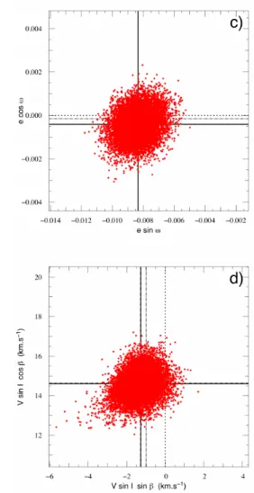
Fig. 7. Fit results for WASP-18b. Nota Bene: Legend similar to the legend in Fig.1.
et al. (2009) presented 9 RV measurements from CORALIE. 28 more have been taken and are presented in this paper. They span over three months. The total data timeseries spans close to 500 days. All RV measurements are presented in the journal of ob-servations at the end of the paper.
Transit timing and geometry were secured by four photomet-ric series: two SuperWASP seasons and two C2 Euler transits in Rband, presented in Hellier et al. (2009).
The fitted data comprises 8593 photometric measurements and 60 radial velocities. Ten free parameters were used, with, in addition, four normalisation constants and two γ velocities.
Eccentricity is clearly detected, improving χ2reduced from 5.58 ± 0.47 to 3.70 ± 0.36 (from 4.31 ± 0.46 to 2.00 ± 0.32 if we remove the RM effect from the calculation). We therefore exclude a circular solution.
The V sin I found in the priorless chain differs from the spec-tral analysis (15.57+1.01−0.69instead of 11 ± 1.5 km s−1), this solution is preferred so as to not produce biased results. For this par-ticular case, we should consider V sin I more like a amplitude parameter in order to fit the Rossiter-McLaughlin effect rather than a bone fide measurement of projected rotation of the star. Therefore, the solution we favour is that of an eccentric orbit, without a prior on the V sin I.
Results are presented in Table. 3, and the best fit is shown in Fig. 7. This Rossiter-McLaughlin effect is one of the largest so
far measured, with an amplitude of nearly 185 m s−1. During the transit sequence O − C = 15.02 m s−1for a mean precision of 6.95 m s−1: the fit is poor; χ2
reduced = 3.70 ± 0.36. This is likely
caused by a misfit of a symmetric Gaussian on a no longer sym-metrical CCF4. We are in fact resolving the planet transit in front
of the star like spots can be detected via Doppler tomography. This has recently been modelled and detected for HD 189733b, as a Doppler shadow by Cameron et al. (2010). The accuracy on the β parameter is not affected by the misfit since it is measured from the asymmetry of the Rossiter-McLaughlin effect. It is in essence estimated from the difference of time spent between the two hemispheres of the star.
Therefore all parameters can be trusted except the V sin I, including the much sought after β angle. We find it to be consis-tent with zero within 1.5 σ: β= −4.0◦+2.5−2.5. The precision on this angle is the best we measured, something that is not reflected in the fit, we therefore doubled error bars to β = −4.0◦+5.0−5.0. This is in part thanks to the brightness of the star, allowing precise measurements of a large amplitude effect. Any departure from the model is quickly penalised in χ2 by the data. Similarly,
ec-centricity is detected above 9 σ with e= 0.00848+0.00085−0.00095thanks 4 this was noted in Triaud et al. (2009) in the case of HD 189733b and CoRoT-3b, but can also be seen on fits of CoRoT-2b (Bouchy et al. 2008), Hat-P-2b (Loeillet et al. 2008) and others.
to the large amplitude of the reflex motion. Note, that fitting ecos ω and e sin ω can correspond to fitting e proportional to e and tending to bias the search for solutions towards higher val-ues. We attempted a few control fits exploring instead √ecos ω & √esin ω. The results showed there is no bias in our analy-sis, so strongly is the eccentricity constrained by the radial ve-locities. The spectroscopic coverage gives us the chance to put some limits on an undetected long term radial velocity drift: | ˙γ| < 43 m s−1yr−1.
The other parameters are consistent with what has been pub-lished by Hellier et al. 2009 and are presented in Table 3.
5. Overall results
Our fits to the Rossiter-McLaughlin effect confirm the presence of planetary spectroscopic transit signatures in all six systems. While three of the six appear closely aligned, the other three exhibit highly-inclined, apparently retrograde orbits. The orbits of all six appear close to circular. Only the massive WASP-18b yields a significant detection of orbital eccentricity.
5.1. Orbital eccentricities
As observed in Gillon et al. (2009b), treating eccentricity as a free fitting parameter increases the error bars on other parame-ters; we are exploring a larger parameter space. One might argue that allowing eccentricity to float is necessary since no orbit is perfectly circular, therefore making an eccentric orbit the sim-plest model available. We argue against this for the simple rea-son that if statistically we cannot make a difference between an eccentric and a circular model then it shows that the eccentric model is not detected. Actually, the mere fact of letting eccen-tricity float biases the result towards a small non zero number, a bias which can be larger than the actual physical value (Lucy & Sweeney 1971). Hence letting eccentricity float when it is not detected is to allow values of parameter space for all parameters to be explored which do not need to be. This is why, unless χ2is
significantly improved by adding two additional parameters to a circular model, we consider the former as preferable. In addition to the risk of biasing, there is a strong assumption that due to tidal effects circularising the planet’s orbit, eccentricities are re-ally small and therefore undetectable for the majority of targets. It is therefore reasonable to assume a value of zero when the data does not contradict it. To facilitate comparison, we also present the results of fits with floating eccentricity. These are given in the appendices; our preferred solutions are described in the text and in table 3.
Only for WASP-18b, have we detected some eccentricity in the orbit, thanks primarily to the high amplitude of the RV signal and the brightness of the target. The amount of RV data taken on WASP-18b is not really more than for the other targets. In addition to a high semi-amplitude, sampling is another key to fixing eccentricity properly. The lack of measured eccentricities on our other targets shows how difficult it is to measure a small eccentricity for these planets as long as no secondary transit is detected to constrain it. Spurious eccentricities tend to appear in fits to data sets where the radial velocities are not sampled uniformly around the orbit, and where the amplitude is small compared to the stellar and instrumental noise levels.
A good example is the case of WASP-17b for which the dou-bling of high precision RV points solely permitted us to place a tighter constraint compared to Anderson et al. (2010).
5.2. Fitting the Rossiter-McLaughlin effect
Our observations yielded results from which five sky-projected spin-orbit angles β have been determined with precision better than 15◦. Three of these angles appear to be retrograde: half our
sample. Adding the two other stars from our original sample that have been published separately (WASP-6b and WASP-8b) we obtain 4 out of 8 angles being not just misaligned but also over 90◦. The precision on the angle depends mostly on the
spec-troscopy as is shown by comparing fits where parameters con-trolled by the photometry are kept fixed (in the appendices).
The error bar on WASP-4b’s β is large. A degeneracy appears when the impact parameter is close to 0 between V sin I and β. The estimate of the spin-orbit angle therefore relies on a good estimate of the stellar rotational velocity as well as with getting a stronger constraint on the shape of the Rossiter-McLaughlin effect. WASP-5b, WASP-17b and WASP-18b are also affected by this degeneracy, with much lower consequences, when the MCMC takes a random step in low impact parameters. This is controlled by the use of a prior on V sin I.
When the planet is large compared to the parent star, or the star rotates rapidly, the cross-correlation function develops a significant asymmetry during transit. This happens because the spectral signature of the light blocked by the planet is par-tially resolved. Fitting a Gaussian to such a profile yields a ve-locity estimate that differs systematically from the velocity of the true light centroid. Winn et al. (2005), and later Triaud et al. (2009) and Hirano et al. (2010) showed how this effect can lead to over-estimation of V sin I. Hirano et al. (2010) have devel-oped an analytic method to compensate for this bias. Cameron et al. (2010) circumvent the problem altogether by modelling the CCF directly, decomposing the profile into a stellar rotation profile and a model of the light blocked by the planet.
Only one star in our sample suffers from this misfit: WASP-18b where easily we see that the value the fit issues for the V sin I is above the estimated value taken via spectral analysis. WASP-17b is the second fastest rotating star. If affected, it is not by much: the fitted V sin I is found within 1 σ of the v sin I .
As shown in Fabrycky & Winn (2009), we can get an idea of the real angle ψ from β by using the following equation, coming only from the geometry of the system:
cos ψ= cos I cos i + sin I sin i cos β (2) where I is the inclination of the stellar spin axis and i the incli-nation of the planet’s orbital axis to the line of sight.
Using the reasonable assumption that the stellar spin axis angle I is distributed isotropically, we computed the above equa-tion using a simple Monte-Carlo simulaequa-tion to draw a random uniform distribution in cos I. We also inserted the error bars on i and β, using a Gaussian random number adjusted to the 1 σ error bars printed in table 5. Fig. 8 shows the transformation from β to ψ for our targets, also illustrating the importance of including error bars in the calculation. We computed the lower ψ (at the 3 σ limit) and found that in the stars we surveyed: WASP-15b is > 90.3◦ and WASP-17b > 91.7◦ therefore retrograde, while WASP-2b is > 89.8◦most probably retrograde.
Statistically we will fail to detect a Rossiter-McLaughlin ef-fect (hence β and ψ) on stars nearly pole-on (with a low I). WASP-2b, with its small V sin I could be a close case. It could be one reason why its RM amplitude is so small (or stellar rota-tion so low). We observe that the spread in ψ is larger than for our other targets.
0 20 40 60 80 100 0.00 0.02 0.04 0.06 0.08 0.10 ψ (o) probability density . . 0 50 100 150 0.00 0.01 0.02 0.03 0.04 ψ (o) probability density . . . . a b c d e f
Fig. 8. top Smoothed histogram of the ψ distribution for WASP-5b. The dotted line is when errors on i and β are set to zero. The plain curve shows the same conversion from β to ψ but with all errors accounted for. bottom: 6 smoothed histograms of the distribution in ψ our six targets: a)-WASP-2b b)-WASP-4b c)-WASP-5b d)-WASP-15b e)-WASP-17b f)-WASP-18b. Bins are of 1◦.
5.3.χ2reduced> 1.
It can be remarked from the text or from the appendices that a few of our objects have χ2reduced > 1.; in the case of WASP-5 notably. This shows the models are not adjusted perfectly to the data. As showcased by model fits to WASP-4, 15 and 17 (with χ2
reduced< 2.) and in many publications using the CORALIE and
HARPS spectrographs, produced error bars on individual radial velocity points are well estimated and understood and worth us-ing as they are (Lovis et al. 2006).
An easy way to solve the problem would be to scale error bars so as to achieve an acceptable χ2. But increasing error bars is not making the model more just; rather, it hides that we do not understand everything: that an extra signal is observed by the instruments; there is information in a bad χ2. Error bars can
be scaled with a value of stellar jitter added quadratically to in-dividual errors, but this applies only if one samples randomly over long periods of time an extra stellar signal. In our case, part of our out-of-transit RVs would feel this jitter, but it would not apply in the same way to the Rossiter-McLaughlin sequences during which we are sensitive to a correlated noise of a different frequency. This renders the increase of error bars prone to errors of judgement, thus leading to a wrong computation of the model.
with the way the data is estimated giving the best optimisation of the data that we could produce using known and substantiated physics. We leave to the reader the assessment of where this ex-tra signal originates from.
5.4. Correlations between parameters
We present a compilation of results from all known observations of the Rossiter-McLaughlin effect in transiting exoplanetary sys-tems in Table 5. No clear correlation is evident between impor-tant planetary parameters such as radii, masses, eccentricities, orbital periods, β and V sin I, except that planets with M < 2 MJ
and e > 0.1 are rare among transiting systems (the only two are Neptunes around M dwarfs); this remark is independent from having a Rossiter-McLaughlin measurement or not. It is hard to see if this is really a result, or a bias due to observations (eg: transits harder to extract from the survey photometry, or to con-firm via radial velocity), or a lack of precision during follow-up making eccentricity hard to detect with confidence. WASP-17b, for example, was previously thought to be the most eccentric transiting planet with M < 2 MJbut our analysis yields only an
upper limit e < 0.110. Eccentricities with as great as e = 0.1 have been published for some planets with masses less that 2MJ,
none of these results are significant at more than the ∼ 2 σ level. The current (Mpsin i, e) distribution in radial velocity does
not show this result, but these masses are only minimum masses. Amongst planets where eccentricity is firmly detected, four out of seven are misaligned. Some of the hot Jupiters appear to be in multiple systems but this appears unrelated to other pa-rameters such as eccentricity or misalignment. Examples are: HD 80606 (Naef et al. 2001), HD 189733 (Bakos et al. 2006), P-1 (Bakos et al. 2007), WASP-8 (Queloz et al. 2010), Hat-P-7 (Winn et al. 2009b), WASP-2, TrES-2 and TrES-4 (Daemgen et al. 2009).
6. Discussion
After a long sequence of closely-aligned planets (Fabrycky & Winn 2009), the sudden appearance of so many misaligned plan-ets is somewhat surprising if not unpredicted. In a collapsing gas cloud, conservation of angular momentum will create a disc from which a star can form. Thus it is expected that star and disc rotate in the same direction with parallel spin axes. If plan-ets form in and migrate through the disc, we can extend the idea that planets’ orbital axes and stellar rotation axes ought to be par-allel. Tides alone cannot make a planet retrograde (Hut 1981). Therefore it is expected that the creation of retrograde planets involves another body: planetary or stellar. Several papers (Wu et al. 2007; Fabrycky & Tremaine 2007; Nagasawa et al. 2008; Chatterjee et al. 2008; Juri´c & Tremaine 2008; Bate et al. 2000, 2009) produce via various processes, orbits which are not copla-nar with the host star’s equator. Of these papers Wu et al. (2007), Fabrycky & Tremaine (2007) and Nagasawa et al. (2008) pro-duce the largest range of angles.
When combining the 26 RM effects that have been observed, we now see that eight planets are severely misaligned: XO-3b (H´ebrard et al. 2008; Winn et al. 2009c) , HD 80606b (Moutou et al. 2009; Pont et al. 2009; Winn et al. 2009a), WASP-14b (Johnson et al. 2009), Hat-P-7b (Winn et al. 2009b; Narita et al. 2009), 8b (Queloz et al. 2010) and 2b, WASP-15b and WASP17b. Of these eight, five have been found to be in retrograde orbits, four from our survey.
0 50 100 150 0 5 10 15 β (o) number . . . . 0 50 100 150 0.0 0.2 0.4 0.6 0.8 1.0 β (o) cumulative probability . . . .
Fig. 9. top: Histogram of all the β measured, binned by 20◦. bot-tom: Cumulative probability function for models by Fabrycky & Tremaine (2007) (blued dashed) and Nagasawa et al. (2008) (red dotted) converted from ψ to β, compared with current obser-vations of β (plain black). The vertical black dotted line shows β = 30◦. Above that, planets are considered misaligned.
Three additional targets may be misaligned: Kepler-8b (Jenkins et al. 2010), 1b (Pont et al. 2010) and CoRoT-3b (Triaud et al. 2009). All three are around faint stars and fairly fast rotators making it hard to determine the angle. All β surements have been plotted in Fig. 9a. Because we only mea-sure the sky-projection of the angle, the planets can in fact be in a variety of configurations. What is their real angle ψ distribution? Deconvolving the whole β distribution into ψ is hypothesis dependent. Hence, to compare the observational data and theo-retical predictions we chose to produce cumulative histograms of observational and theoretical β angles in Fig. 9b. We transformed predictions from Fabrycky & Tremaine (2007) and Nagasawa et al. (2008), by taking their ψ histograms and transforming them geometrically into observable β, with the assumption that I is isotropic. For a fixed ψ, we define an azimuthal angle α mea-sured from a zero point where the star’s north pole is tilted to-wards the observer. If we precess the star for α ∈ [0, 2π[ we obtain β via a Monte Carlo simulation from solving:
tan β ' tan ψ sin α (3)
using the conservative assumption that i = 90◦since these
sys-tems are transiting.
Results from this transform are in Fig. 9b. The observational data has been overplotted. Both observations and models by Fabrycky & Tremaine (2007) agree that about 55 % of planets should appear with β < 30◦5. Overall the theoretical distribution
is a little steeper than the observations. We clearly remark that predictions by Nagasawa et al. (2008) agree in range but not in the shape of distribution of observed β, notably, it lacks enough aligned systems. This model is handy to illustrate the difference between the observations and a distribution isotropic in ψ.
Disc migration models would only produce a steep distribu-tion reaching unity before 30◦. A combination of several models is not attempted here because of the vast amount of possibilities and the likelihood that models will evolve.
The theoretical ψ distribution published by Fabrycky & Tremaine (2007), transformed into β, shown along the angle dis-tribution obtained from observations, in Fig. 9b gives a remark-ably close match. If the form of this distribution is borne out by future observations, we may then conclude that hot Jupiters are formed by this very mechanism. Wu et al. (2007) predictions are essentially the same as those from Fabrycky & Tremaine (2007). We also attempted to generalise the method explained in sec-tion 5.2 to all objects presented in table 5: we are going to as-sume two distributions for the stellar spin axis in order to derive a distribution of real obliquity ψ. Two hypotheses were checked. The first was to assume an isotropy of the stellar axis angle I by taking a uniform distribution in cos I from 0 to 1; the second was to assume stellar axes are aligned with the plane of the sky. For this last hypothesis we assumed all cos I followed a Gaussian distribution centred on 0 with a variance of 0.1, an error bar cor-responding to the best of what observations can give us at the moment to constrain the stellar I. Taking these hypotheses al-lows to test for extremes and get an idea of the true proportion of misaligned planetary systems.
The first hypothesis is shown on Fig. 10 plotted in compar-ison with the theoretical predictions by Fabrycky & Tremaine (2007). Inferring an isotropic distribution in stellar axes gives us as an upper bound that 86.2 % of the probability density dis-tribution is at ψ > 30◦. The other hypothesis gives a
propor-tion of 43.6 % of misaligned systems. The effect of constrain-ing the stellar I makes every individual contribution narrower in range. Taking a stricter constraint does not change this propor-tion much.
Both hypotheses are at the extremes of what the real distri-bution of I is. We interpret these results as showing that between 45 and 85 % of systems are misaligned with ψ > 30◦. Aligned systems are no longer the norm, radically altering our view on how these hot Jupiters formed.
Fabrycky & Tremaine (2007) and Wu et al. (2007) use the Kozai mechanism (Kozai 1962; Wu & Murray 2003) induced by an outer binary companion to the inner planet, to move the planet from the ice line where it is thought to form, to the in-ner stellar system. As the planet gets closer to the primary, tidal friction helps to break the Kozai cycles and finalise the planet’s orbital parameters. Their equations are extracted from work by Eggleton & Kiseleva-Eggleton (2001). The resulting ψ distribu-tion extends from 0◦up to 150◦away from the primary’s rotation axis (see Fig. 10). In this scenario, the planet can be created in a binary star system, or around a single star which acquired a
5 this criterion of misalignement of β > 30◦
, is a limit where, with current error bars on β, one can generally have a significant detection of a misalignement.