Lisbon, Portugal, 5–9 June 2006
STRESS CONSTRAINED OPTIMIZATION USING X-FEM AND LEVEL
SET DESCRIPTION
L. Van Miegroet1, T. Jacobs1−2, E. Lemaire1and P. Duysinx1
1University of Li`ege
Automotive Engineering / Multidisciplinary Optimization LTAS Aerospace and Mechanics Department
Chemin des Chevreuils, 1, building B52, 4000 Li`ege, Belgium e-mail:{L.VanMiegroet, E.Lemaire, P.Duysinx}@ulg.ac.be
1−2Formerly 1, currently 2 Universit´e Laval Qu´ebec D´epartement de G´enie civil
Pavillon Adrien-Pouliot Universit´e Laval (Qu´ebec) Canada e-mail: [email protected]
Keywords: Shape optimization, X-FEM, Level Set.
Abstract. This paper presents and describes an intermediate approach which takes its place
between the two classical methods of shape and topology optimization. It is based on using the recent Level Set description of the geometry and the novel eXtended Finite Element Method (X-FEM). The method benefits from the fixed mesh work using X-FEM and from the curves smoothness of the Level Set description. Design variables are shape parameters of basic ge-ometric features. The number of design variables of this formulation remains small whereas various global and local constraints can be considered. A key problem which is investigated here is the sensitivity analysis and the way it can be carried out precisely and efficiently. Nu-merical applications revisit some classical 2D (academic) benchmarks from shape optimization and illustrate the great interest of using X-FEM and Level Set description together. The paper presents the results of stress constrained problems using the proposed X-FEM and Level Set based formulation. A central issue is the sensitivity analysis (related to the compliance and/or the stresses) and the way it can be carried out efficiently. A special attention is also paid to stress constrained problems which are often neglected in other Level Set Methods works.
1 INTRODUCTION
Topology optimization has experienced an incredible soar since the seminal work of Bendsøe and Kikuchi [2] and is now available within several commercial packages and finite element codes. It is used with great success in industrial applications. Practically, one major advantage of the optimal material distribution formulation is to be able to work on a fixed regular mesh. The drawback is that this formulation comes to very large scale optimization problems, so that one generally considers very simple design problems as the minimum compliance problem with a single volume constraint. Introducing local constraints can lead to problems that are hugely difficult to handle, whereas controlling geometrical constraints, which are mainly related to manufacturing considerations, requires some sophistications. Finally the optimal structure picture needs to be interpreted to construct a parametric CAD model.
Meanwhile, shape optimization had received attention since the beginning of the eighties, but remain quite unsuccessful in industrial applications. Nevertheless, shape optimization of internal and external boundaries is of great interest to improve the detailed design of structures against many criteria as restricted displacements or stress criteria. The shape optimization in-troduces a few design variables since the design problem is formulated on the parameterized CAD model level. The major difficulty is related to the mesh management problems coming from the large shape modifications. Mesh distorsions and Finite Element errors can be reduced using remeshing between two iterations and mesh adaptation tools. However a major technical problem also stems from the sensitivity analysis that requires the calculation of the so-called ve-locity field because of the moving mesh. It turns out that shape optimization remains generally quite fragile and delicate to use in industrial context.
In order to circumvent the technical difficulties of the moving mesh problems, a couple of researches have tried to formulate shape optimization with fixed mesh analyses using fictitious domains as in Ref. [6], based on fixed grid finite elements in Ref. [8] or more recently using projection methods as in Ref. [9]. The present work relies on the novel eXtended Finite
El-ement Method (X-FEM) that has been proposed as an alternative to remeshing methods (see
Ref. [3] or [4] for instance). The X-FEM method is naturally associated with the Level Set [11] description of the geometry to provide a very efficient treatment of difficult problems involving discontinuities and propagations. Up to now the X-FEM method has been mostly developed for crack propagation problems [3], but the potential interest of the X-FEM and the Level Set de-scription for other problems like topology optimization was identified very early in Belytschko et al. [5], while the advantages of the Level Set method in structural optimization was clearly demonstrated by Wang et al. [14] or Allaire et al. [1].
The authors see the X-FEM and the Level Set description as an elegant way to fill the gap between topology and shape optimization. The method can be qualified as generalized shape
optimization as it has smooth boundary descriptions while allowing topology modifications as
holes can merge and disappear. X-FEM enables working on a fixed mesh, as in topology op-timization, circumventing the technical difficulties of shape optimization. The structural shape description uses basic Level Set features (circles, rectangles, etc.) that can be freely combined to generate any shapes. The design variables are parameters of the Level Set features, while constraints can be either global (compliance, volume) or local (stresses) responses as in shape optimization. A key issue for this problem is the sensitivity analysis. A semi analytical ap-proach has been developed for the compliance, the displacements and the stresses. The work presents clearly validated solutions and still open questions and difficulties. For the numerical applications a complete solution of shape optimization using Level Set description and X-FEM
has been implemented in the object oriented software, OOFELIE (Open Object Finite Element Lead by Interactive User) [10].
The layout of the paper is thus the following. The Extended Finite Element Method, the Level Set representation and the interaction between these two methods are reminded in sections 2 and 3. Section 4 states the formulation of optimization problem and difficulties introduced by the X-FEM and the Level Set description. Sensitivity analysis is addressed in section 5. Finally in section 6 the applications are presented to illustrate the proposed extended finite elements and their application to generalized shape optimization.
2 THE EXTENDED FINITE ELEMENT METHOD
Up to now the eXtended Finite Element Method [3, 4] has been mainly developed for crack propagation problems, but the interest of the X-FEM and Level Set methods possess large
po-tential for further application fields. Hence, Belytschkoet al (see [5]) identified very early the
potential of these methods for shape and topology optimization.
The main strength of the X-FEM method is its capability to allow discontinuities inside the finite elements. Hence, this one enables to include geometric boundaries, cracks, material or phase changes that are not coincident with the mesh and avoid the expensive mesh regeneration for crack evolution problems.
2.1 The basis of the method
In the classical Finite Element Method, it is not possible to model a discontinuity inside an
element because the trial shape functions used are required to be at leastC1. Then, in order to
model a type of discontinuities inside the elements and therefore to be able to represent discon-tinuities in the physics fields, it is necessary to add special shape functions to the finite element approximation. Hence, in the case of cracked structures, the displacement is the discontinuous field and the modelisation of this field needs therefore to possess discontinuous shape func-tions in order to represent it precisely. The classical finite element approximation used is then extended to embed the discontinuous shape function as in the following equation:
u(x) =X i uiNi(x) + X j ajNj(x)H(x) (1)
in this expression,Ni(x) are the classical shape functions associated to degrees of freedom ui.
The Nj(x)H(x) are the discontinuous shape functions constructed by multiplying a classical
Nj(x) shape function with a Heaviside function H(x) (presenting a switch value where the
discontinuity lies). Note that this set of extended shape functions are only supported by the
enriched degrees of freedomaj. Morevover, only the elements near the discontinuity usually
support extended shape functions whereas the other elements remain unchanged (i.e. classical FE). The modification of the displacement field approximation does not introduce a new form of the discretised finite element equilibrium equation but leads to an enlarged problem to solve (see Ref. [4] for details):
K· q = g ⇔ " Kuu Kua Kau Kaa # " u a # = " fext u fext a # (2) As the elements can now present discontinuous shape functions, the numerical integration scheme has to be modified in order to take care of the discontinuity. In our implementation, the elements embedding a singularity are divided into sub-triangular elements aligned with this
2.2 Representing holes
The modeling of material-void interfaces with X-FEM [12] differs only marginaly from the cracked structure case. Hence, for void inclusions and holes, the displacement field is now approximated by: u(x) =X i uiNi(x)V (x) (3) where V (x) = ( 1 if x ∈ material zone 0 if x ∈ void zone ) (4)
One can note that this functionV models perfectly the singularity presented inside the
displace-ment field as this function imposes a value zero when oustide the material (see Fig. 1).
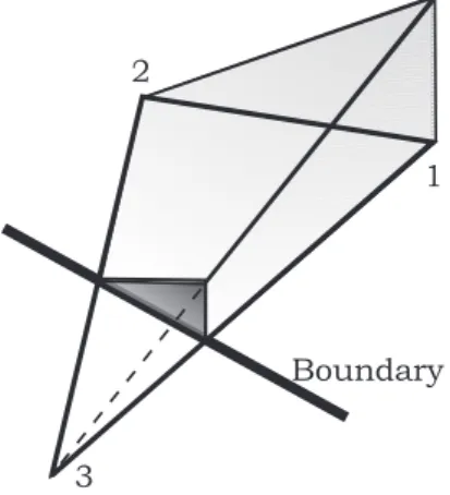
Boundary
3 2
1
Figure 1: Representation of the shape function of node 1 on a cut element
The elements lying fully outside the material are removed from the system of equations, whereas the partially filled elements are integrated using the X-FEM integration procedure over solid sub-domain (see Fig. 2). Consequently, the size of the problem is not augmented regard-ing to a finite element model.
void
solid Boundary
Figure 2: Sub-division of a quadrangular element and Gauss points
Modeling holes with the X-FEM is a very appealing method for the shape optimization but also for the topology optimization as no remeshing is needed and no approximation is done on the nature of the voids in opposition to the power penalization of intermediate densities method used in topology optimization (SIMP). However, the X-FEM method needs more complicated integration procedure and elements.
3 THE LEVEL SET DESCRIPTION
The explicit representation of the structural shape of parametric CAD representation forbids deep boundary or topological changes such as creation or fusion of holes. This limitation is one of the main reasons of the low performance generally associated to the shape optimization. Conversely, the Level Set method developed by Sethian [11] which consists of representing the boundary of the structure with an implicit method allows this kind of deep changes.
The Level Set method is a numerical technique first developed to track moving interfaces. It is based upon the idea of implicitly representing the interfaces as a Level Set curve of a higher
dimension functionψ(x, t). The boundaries of the structure is then conventionally represented
by the zero level i.e. ψ(x, t)=0 of this function ψ, whereas the filled region is attached to the
positive part of theψ function. In practice, this function is approximated on a fixed mesh by a
discrete function which is usually the signed distance function to the curveΓ:
ψ(x, t) = ± min
xΓ∈Γ(t)
kx − xΓk (5)
ψ(x, t) > 0 ⇔ Solid
ψ(x, t) < 0 ⇔ V oid (6)
The sign is positive (negative) if x is inside (outside) the boundary defined byΓ(t). Applied
to the X-FEM framework, the Level Set is defined on the structural mesh and a geometrical degree of freedom representing its Level Set function value is associated at each element node. The Level Set is then interpolated on the whole design domain with the classical shape function of the finite element approximation:
ψ(x, t) =X
i
ψiNi(x) (7)
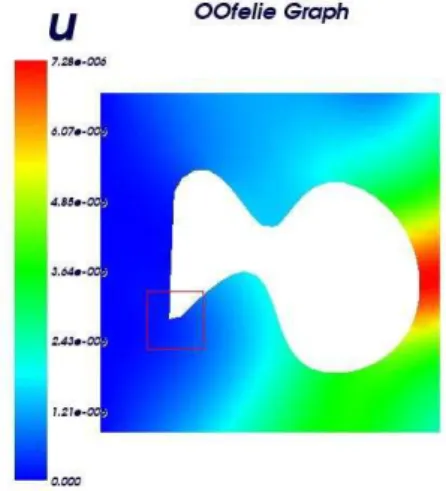
The combination of different Level Sets is also one of the appealing characteristic of this method. This property allows easy treatment of merging interfaces and connectivity modifica-tions. However one drawback of the Level Set description lies in the difficulties encountered in representing sharp corners with a rather coarse mesh as shown on the figure 4 (b). This one also illustrates the use of a Level Set for the description of the internal boundaries of an X-FEM model.
0.361 0.361 0.264 0.264 0.168 0.168 0.07120.0712 -0.0252-0.0252 -0.122-0.122 -0.218-0.218 Level Set Level Set OOfelie Graph OOfelie Graph
(a) Level Set representation of NURBS curve (b) Displacement of the X-FEM model
Figure 4: Geometric representation and X-FEM displacement result
To deal with this inherent problem, two solutions exist:
1/ increase the refinement of the mesh, which can be very expensive in terms of CPU cost for the X-FEM resolution.
2/ use a higher order of shape functions in order to interpolate the Level Set boundary with more accuracy inside the elements.
Inside the cut elements, the Level Set is interpolated linearly when first order finite element are used. As a consequence, the representation of the boudaries can overestimate or underesti-mate the surface (volume) of the structure. Hence, the estimation of the surface depends on the number of cut elements, on the position of the inteface inside the element and of course on the mesh refinement. To illustrate this phenomenon, we have computed the variation of the surface with respect to the position of a hole on a square plate (Fig. 5). This error can causes some ”zigzagging” problems during optimization if one uses a very coarse mesh and a constraint or objective function related to the area (volume).
(a) Surface of the plate (b) Isovalue of the surface
4 FORMULATION OF OPTIMIZATION PROBLEM
The formulation of the considered optimization problem is similar to that of a shape opti-mization problem, but its solution is greatly simplified thanks to the use of the X-FEM and Level Set description as no velocity field and mesh perturbation are needed.
The geometry and the material repartition are specified using Level Sets representations. The positive part of the Level Set represents the region where lies the material and the negative part the void. The user has a library of basic geometric features (in Level Sets) that can be combined to create almost any structural geometry. The available geometric features are circles, ellipses and all polygons. The design variables are chosen among the geometric parameters of these features.
The optimization problem aims at finding the best shape for minimizing a given objective function while satisfying mechanical and geometrical design restrictions. The mechanical con-straints can either be global responses (e.g. compliance, volume) or local ones such as displace-ments or stress constraints.
The number of design variables is generally small as in shape optimization. However the number of constraints may be large if many local stress restrictions (e.g. stress constraints) are considered. Nonetheless, large scale problems as in topology optimization are avoided.
The design problem is stated as a general constrained optimization problem: min x g0(x) s.t.: gj(x) ≤ gjmax j = 1 . . . m xi ≤ xi ≤ xi i = 1 . . . n (8)
The solution to this problem is obtained using the so-called sequential convex programming. At each iteration, the X-FEM analysis problem is solved and a sensitivity analysis is performed. The solution of the optimization problem is then found by using a CONvex LINearization ap-proximation scheme of each constraint functions (CONLIN [7]). The solution becomes the new design and the procedure is repeated until convergence.
Because of the X-FEM characteristics, the geometry has not to coincide with the mesh and the shape optimization problem is carried out on a fixed mesh. One works here in an eulerian approach and not in a lagrangian approach. This circumvents the mesh perturbation problems of classical shape optimization. Sensitivity analysis does not require the velocity field anymore. The present formulation is then, up to a certain point, simpler. However, some technical difficul-ties can be encountered if a finite difference or a semi-analytical scheme is used for sensitivity analysis as explained in the next section. Basically, the problem is that the perturbation must not change the number of degrees of freedom of the X-FEM stiffness matrix.
The Level Set approach is very convenient to modify the geometry because the Level Sets (and so the holes) can penetrate each other or disappear. Creation of new holes is more prob-lematic since it leads to a non smooth problem. Topological derivatives have then to be used for a rigorous treatment of the problem. This capability has not been implemented in this study.
5 THE SENSITIVITY ANALYSIS METHOD
As in classical shape optimization, the sensitivity analysis of mechanical responses (such
as compliance, displacement, stress,. . .) is carried out using a semi-analytic approach. In this
differences with respect to a small perturbationδx of Level Set parameters: ∂K ∂x ≃ K(x + δx) − K(x) δx (9) ∂f ∂x ≃ f(x + δx) − f (x) δx (10)
These derivatives are then used to compute the sensitivity of the various objective functions. To illustrate the procedure, consider the discretized equilibrium equation and the expression of the
complianceC: C = 1 2u TKu (11) Ku = f (12)
In the case of invariant loading forces, the expression of the generalized displacements
sensitiv-ity allows the derivative of the complianceC to be expressed as a function of the siffness matrix
derivative: ∂u ∂x = K −1(−∂K ∂xu) (13) ∂C ∂x = − 1 2u T∂K ∂xu (14)
Now, if the objective function or constraint involves the stresses of the problem, the sensitivity of this response is needed. Two basic methods are available to get the derivative of the stresses. The first one, which has the drawback of being very arduous, consist in derivating the expression of the stresses (σ) in all the elements:
σ = HBju (15)
where H is the local Hooke’s matrix and Bj the matrix of the derivated shape functions of
the element j. The second method is based on the computation of the stresses related to the
perturbated state by using the expression of the displacement sensitivities:
σ(x) = HBju(x) (16) σ(x + δx) ≃ HBju(x + δx) (17) ∂σ ∂x ≃ σ(x + dx) − σ(x) ∂x (18)
This procedure reduces the sensitivity of the stresses as a function of the displacement deriva-tive. In the present paper, it is this second method which has been implemented.
In the classical shape optimization, the computing complexity of the stiffness matrix
sensitiv-ity is due to the modifications of the mesh associated to the perturbationδx and to the velocity
field calculation. In the present X-FEM based approach, one has not to deal with the mesh perturbations as one works on a fixed grid. However, this method exhibits a different draw-back with respect to the general shape optimization as the number of elements may change. The critical situation happens when the Level Set is very close to a node (see Fig. 6). Thus,
during the perturbationδx of the Level Set, there is a possibility of previously empty element
introduce some new nodes and their unknown displacements. Therefore, the number of degrees of freedom change and the dimension of the stiffness matrix is modified between the Level Set perturbation. However, this situation is extremely unusual for free mesh used in practice but the problem deserves our attention to be treated correctly.
The strategy that is implemented presently to circumvent the difficulty is the following. As
one has only the displacement (ui) for the elements that are present in the reference
configura-tion, only these elements are taken into account while the contributions coming from the new partly filled elements are ignored. Hence, no new elements are introduced and the size of the stiffness matrix remains unchanged. Of course, the ultimate solution to the problem should resort to a fully analytical sensitivity of the stiffness matrix. However, this would be rather restrictive for industrial applications.
(a) Reference Level Set and mesh (b) Perturbated level set
Figure 6: Sensitivity difficulty with semi-analytic approach
An error is obviously introduced by this strategy because the contributions related to new created elements are ignored. However, in practice, the contribution of these elements would remains so small that the neglected contribution to the stiffness matrix would not have any sig-nificant effects on the accuracy of the sensitivity. The quality of the approximation is illustrated in the application section with the elliptical hole problem.
On-going work has already singled out three further strategies to reduce the error of the semi-analytic approach:
1/ One can keep a narrow band (boundary layer) of elements with very soft mechanical
properties around the Level Set ψ = 0 in order to prevent the variation of the total number of
degrees of freedom.
2/ One could define a tolerance zone around the Level Set. If the discontinuity in an element lies inside this zone, add the connected elements to the set of cut ones.
3/ One could remark that when one element is created, in fact only one node is added to the formulation as depicted on the figure 7 (e.g. the node 4). Hence, one could take into account a part of the contribution of this new element by only reporting to the global stiffness matrix the terms involving the nodes already present.
(a) Initial geometry (b) Final geometry Figure 7: Node added to the formulation
The elementary stiffness matrix of triangle 1 and 2 are defined by:
K∆1 = k∆1 11 k12∆1 k13∆1 k∆1 21 k22∆1 k23∆1 k∆1 31 k32∆1 k33∆1 K∆2 = k∆2 22 k∆232 k∆242 k∆2 32 k∆332 k∆342 k∆2 42 k∆432 k∆442 (19) wherek∆k
ij is a component of the stiffness matrix modelling the link between nodei and j in
trianglek. The global matrix of the whole problem is for the initial step:
Kglobal∆1 = k∆1 11 k12∆1 k13∆1 k15 k∆1 21 k22∆1 k23∆1 k25 k∆1 31 k32∆1 k33∆1 k35 k51 k52 k53 k55 . .. (20) (21) and, for the perturbated step:
Kglobal∆1+∆2 ≃ k∆1 11 k12∆1 k13∆1 k15 k∆1 21 k∆221 + k∆222 k∆231 + k∆232 k25 k∆1 31 k∆321 + k∆322 k∆331 + k∆332 k35 k51 k52 k53 k55 . .. (22)
The terms related to the node 4 are then missing in the perturbated stiffness matrix but a part of the triangle 2 stiffness is however taken into account by the terms related to node 3 and 2. Moreover, one can also note that these terms should be more important than the terms involving the node 4 as the element is filled in the region surrounding node 2 and 3.
The first two alternative methods have the advantages of keeping the number of degrees of freedom constant and forbid the creation of elements during the perturbation step. Hence, the computation of the sensitivity would lead to a more accurate result as all elements are taken into account in the perturbated stiffness matrix. However, the presence of these elements is expected to introduce a dependency upon the mechanical properties associated to the narrow softening
elements band like in topology optimization with the power p coefficient in the SIM P law.
Moreover, using these methods does not take fully advantage of the X-FEM as we re-introduce an approximation of the void as a weak material. The last method seems to be very attractive as this advantage is kept for the modelisation of the void. However, a very small error will remain but is believed not to affect the problem description and can therefore be neglected.
6 APPLICATIONS
The X-FEM method for the modelisation of material-void discontinuity and its Level Set description have been implemented in an object oriented (C++) multiphysics finite element code, OOFELIE that is commercialized by Open Engineering [10].
In OOFELIE, any mechanical result can be chosen as objective functions and constraints that is: compliance and potential energy, all stress components, displacements and geometric results. Presently, implementation of the X-FEM method is available in 2-D problems with a library of both quadrangle and triangle elements. The Level Set description can be defined different ways. They can be constructed classicaly from functions or from a set of points which are interpolated by a NURBS curve. However in this study, solely parameters of the functions can be used as optimization variable. Further work is needed in order to test optimization with the control points of the NURBS. The CONLIN optimizer by C. Fleury [7] has also been coupled in the OOFELIE environment and an optimization framework has been created.
6.1 Plate with an elliptical hole
The plate with a hole is a classical benchmark from shape optimization. To remind the reader, a large plate with a hole in the middle is subjected to a biaxial stress field. The goal of the optimization problem is to find the optimal shape to minimize the compliance of the structure with a constraint on the total surface of the hole. From the analytical solution, we know that the solution is an elliptical hole aligned with the principal stresses.
OOfelie Graph
OOfelie Graph
(a) Initial geometry
OOfelie Graph
OOfelie Graph
(b) Final geometry Figure 8: Plate with an elliptical hole
Here particular values are considered. The dimensions of the plate are 2× 2 × 1 m. The domain
is covered with a transfinite mesh with 30 nodes on each side. The applied biaxial stress field
is σx=2σ0 andσy=σ0. The material properties associated are: Young modulus E = 1 N/m2,
Poisson’s rationν=0.3. The plane stress state is assumed. The variables are the angle θ and
the long axis a. Figure 8 left shows the initial design domain, an elliptic hole with a 45◦
orientation. Three iterations with CONLIN optimizer are necessary to come to the solution, an ellipse aligned with the principle stresses (see Fig. 8(b)).
Let’s remark the discretization of the geometry using the level set. The boundaries are rep-resented using the linear finite element shape functions, so that the boundary is approximated using piecewise linear segments. This can lead to discretization errors of the geometry as noted in [13] and in section 3.
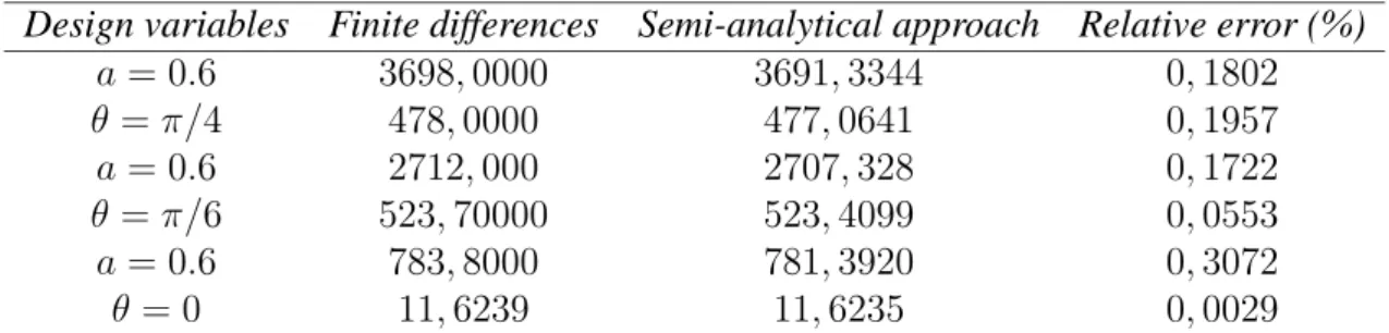
Design variables Finite differences Semi-analytical approach Relative error (%)
a = 0.6 3698, 0000 3691, 3344 0, 1802 θ = π/4 478, 0000 477, 0641 0, 1957 a = 0.6 2712, 000 2707, 328 0, 1722 θ = π/6 523, 70000 523, 4099 0, 0553 a = 0.6 783, 8000 781, 3920 0, 3072 θ = 0 11, 6239 11, 6235 0, 0029
Table 1: Validation of semi-analytical sensitivity analysis approximation.
The elliptical hole also serves as a tool for the validation of the approximated semi-analytical sensitivity analysis that has been proposed in section 5. Table 1 gives the sensitivities of com-pliance calculated by finite differences and semi-analytical approach for different combinations
of the design variables a and θ. The results were obtained with a relative perturbation of the
design variables ofδ = 10−4. The table presents the quality of the proposed semi-analytical
approximation.
6.2 Plate with a generalized superelliptical hole
Several works have also been devoted to shape optimization of more complicated kind of holes (see Ref. [15]). One of these is the superellipse which is a generalization of the classical
ellipse. The generalized superellipse is a superellipse for which the two exponentα and η can
be different and has following expression: ¯ ¯ ¯ ¯ x a ¯ ¯ ¯ ¯ α + ¯ ¯ ¯ ¯ y b ¯ ¯ ¯ ¯ η = 1 (23)
Figure 9 presents some superellipses for the case ofα=η.
−5 −4 −3 −2 −1 0 1 2 3 4 5 −3 −2 −1 0 1 2 3 η=α=0.7 η=α=1 η=α=2 η=α=4 η=α=8
The second application presented is also a plate with a hole, but in this case, a superelliptical
hole. Figure 10 right shows the initial quarter design domain, a superellipse with valuesα=β=4,
a=6, b=4 and an orientation angle equal to zero.
OOfelie Graph
OOfelie Graph
(a) Initial configuration of the superellipse
OOfelie Graph
OOfelie Graph
(b) Final configuration Figure 10: Superellise initial and final design
Here the particular values are considered. The dimensions of the plate are 8× 8 × 1 m. The
domain is covered with a delaunay mesh with 26 nodes on each side. The applied biaxial
stress field is σx=σ0 and σy=σ0 and the material properties associated are: Young modulus
E = 2.1e11 N/m2, Poisson’s rationν=0.3. The plane stress state is assumed. The variables are
the two exponentsα, β and the long and small axis a, b. The exponents are restricted to values
between 2 and 8 whilea and b are constrained between 2 and 8. The objective function consists
in minimizing the compliance with an upper bound on the volumeV .
OOfelie Graph OOfelie Graph Iteration nb Iteration nb 0.000 0.000 3.00 3.00 6.00 6.00 9.00 9.00 12.0 12.0 15.0 15.0 Obj Fct Obj Fct 193. 193. 173. 173. 153. 153. 133. 133. 113. 113. 93.0 93.0
Figure 11: Evolution of the objective function for the superellipse case
Fourteen iterations were necessary with CONLIN optimizer to reach the solution (see Fig
mainly due to the form of the volume constraint which significantly reduces the advancing step of the optimization due to the approximation of the constraint.
6.3 Stress constrained optimization
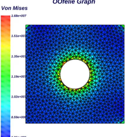
The third application presented is similar to first one as we also use an ellipse. The right hand side of figure 12 shows the initial design domain.
OOfelie Graph OOfelie Graph Von Mises Von Mises 6.92e+006 6.92e+006 9.37e+006 9.37e+006 1.18e+007 1.18e+007 1.43e+007 1.43e+007 1.67e+007 1.67e+007 1.92e+007 1.92e+007 2.16e+007 2.16e+007
(a) Initial geometry
OOfelie Graph OOfelie Graph Von Mises Von Mises 6.96e+006 6.96e+006 8.59e+006 8.59e+006 1.02e+007 1.02e+007 1.19e+007 1.19e+007 1.35e+007 1.35e+007 1.51e+007 1.51e+007 1.68e+007 1.68e+007 (b) Final design Figure 12: Evolution of the geometry
In a similar fashion to that of the previous two applications, the problem is defined by the
following characteristics : plate dimensions (1× 1 × 1 m), delaunay mesh with 28 nodes on
each side, biaxial stress fieldσx=σ0 andσy=σ0, E=2.1e11 N/m2,ν=0.3. The plane stress state
is assumed. The variables are the axis a and b and the value of the angle θ related to the axis
x. The objective function consist in minimizing the compliance with a maximum value for the
volumeV and an upper bound of 80% on the inital maximum Von-Mises stress.
OOfelie Graph OOfelie Graph Iteration nb Iteration nb 0.000 0.000 3.00 3.00 6.00 6.00 9.00 9.00 12.0 12.0 15.0 15.0 Obj Fct Obj Fct 1.74e+003 1.74e+003 1.71e+003 1.71e+003 1.68e+003 1.68e+003 1.65e+003 1.65e+003 1.62e+003 1.62e+003 1.59e+003 1.59e+003
Figure 13: Geometric representation and X-FEM displacement result
configuration is presented on the figure 12(b). As one can notice, the final solution respects the constraint imposed on the initial maximum Von-Mises Stress reduction even if the initial model was considered as infeasible by the optimizer because of the constraint violation.
7 CONCLUSIONS
In this paper, an novel approach based on the Level Set description and the X-FEM for the mechanical optimization of structures has been presented. This new method takes place between shape and topology optimization as it possesses the main advantages of this two ones. The X-FEM method has proven to be very useful as it easily takes advantage of the fixed mesh work approach of topology optimization whereas the smooth curve description from the shape optimization is kept. Moreover, void is not approximated as a smooth material in opposition to the SIMP method. Finally, no remeshing process is needed in our applications contrary to shape optimization.
The investigation of a semi-analytic sensitivity analysis with X-FEM and Level Set is an original contribution to the paper as is the use of stress constraints. Up to now, a sensitivity analysis procedure has been developed for the displacements, the compliance and the stresses. The problem of elements becoming partially filled has been identified and a first strategy to cir-cumvent the problem has been validated. On-going work explores other alternative approaches. The solution of 2-D problems is presently available. Future work is devoted to attack 3-D problems, dynamic problems, and multiphysic (electro-mechanical) problems.
8 ACKNOWLEDGMENTS
The authors gratefully acknowledge the support of project ARC MEMS, Action de recherche concert´ee 03/08-298 funded by the Communaute Francaise de Belgique and by project RW 02/1/5183, MOMIOP funded by the Walloon Region of Belgium for this research.
REFERENCES
[1] Allaire G. Jouve F. and Toader A.M. (2004) Structural optimization using sensitivity anal-ysis and a level-set method. Journal of Computational Physics. Vol. 194, Issue 1, pp 363-393.
[2] Bendsøe M. P. and Kikuchi N. (1988). Generating Optimal Topologies in Structural De-sign Using a Homogenization Method, Computer Methods in Applied Mechanics and
En-gineering, 1988, 71, 197-224.
[3] Moes N., Dolbow J., Sukumar N. and Belytschko T. (1999) A finite element method for crack growth without remeshing. International journal for numerical methods in
engi-neering 1999, no. 46, 131-150.
[4] Belytschko. T. Parimi C. , Moes N. , Sukumar N. and Usui. S. (2003). Structured extended finite element methods for solids defined by implicit surfaces. Int. J. Numer. Meth. in
Engng 2003; 56 : 609-635.
[5] Belytschko T., Xiao S. and Parimi C. (2003). Topology optimization with implicit func-tions and regularization. Int. J. Num. Meth. in Engng 2003; 57 : 1177-1196.
[6] Dankova J. and Haslinger J. (1996) Numerical realization of a fictitious domain approach used in shape optimization. Part I Distributed controls. Applications of Mathematics 1996, 41(2): 123-147.
[7] Fleury C. (1989) CONLIN: an efficient dual optimizer based on convex approximation concepts. Structural Optimization. Vol. 1, pp 81-89.
[8] Garcia-Ruiz M.J. and Steven G.P. (1999) Fixed grid finite element in elasticity optimiza-tion. Engineering Computations 1999, 16(2): 145-164.
[9] Norato J., Haber R., Tortorelli D. and Bendsøe M.P. (2004) A geometry projection method for shape optimization. Int. J. Num. Meth. in Engng 1999, 60(14): 2289-2312.
[10] OOFELIE, an Object Oriented Finite Element Code Led by Interactive Execution. Internet resources: www.open-engineering.com.
[11] Sethian J. (1999) Level Set Methods and Fast Marching Methods: Evolving Interfaces
in Computational Geometry, Fluid Mechanics, Computer Vision and Materials Science,
Cambridge University Press, 1999.
[12] Sukumar N., Chopp D. L., No¨es N. and Belytschko T. (2001) Modelling holes and inclu-sions by Level Set in the extended finite element method. Comput. Methods Appl. Mech.
Engrg. 2001, 190, pp 6183-6200
[13] Van Miegroet L., Moes N., Fleury C. and Duysinx P. (2005). Generalized shape optimiza-tion based on the Level Set method. Proceedings of the 6th World Congress of Structural and Multidisciplinary Optimization (J. Herskowitz ed.), Rio de Janeiro, Brazil, May 30 -June 3 2005.
[14] Wang M., Wang X. and Guo D. (2003). A Level Set method structural topology optimiza-tion. Comp. Methods in Appl. Mech Engng. 2003; 191:227-246.
[15] Pedersen P. (1991). Optimal shape design with anisotropic materials. NATO/DFG ASI Proceeding of vol. 1 Optimization of Large Structural Systems (Dir. G. Rozvany), Bercht-esgaden, Germany, Sept. 23 - Oct.4 1991.