1
The semantic map model
State of the art and future avenues for linguistic
research
Abstract. The semantic map model is relatively new in linguistic research, but it has been intensively used during the past three decades for studying both cross-linguistic and language-specific questions. The goal of the present contribution is to give a comprehensive overview of the model. After introducing the different types of semantic maps, we present the steps involved for building the maps and discuss in more detail the different types of maps and their respective advantages and disadvantages, focusing on the kinds of linguistic generalizations captured. Finally, we provide a thorough survey of the literature on the topic and we sketch future avenues for research in the field.
1
| INTRODUCTION: WHAT IS A SEMANTIC MAP?
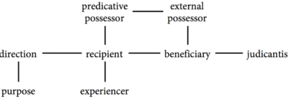
This paper provides an overview of the semantic map model, a relatively new approach in linguistic research. The model has been intensively used during the past three decades for studying both cross-linguistic and language-specific questions. A semantic map is a way to visually represent the interrelationships between meanings1 expressed in languages. One can distinguish two types of semantic maps: classical maps and proximity maps (van der Auwera, 2013; see Sections 4 and 5 respectively for alternative labels). Classical semantic maps typically take the form of a graph —with nodes standing for meanings and edges between nodes standing for relationships between meanings. Figure 1a is a textbook example of a classical semantic map for dative functions.
FIGURE 1a Semantic map of dative functions (adapted from Haspelmath, 2003: 213)
In such maps, two meanings are connected if they are expressed by the same linguistic item in at least one language. These maps are inferred from typological 1 Throughout this paper, we use the neutral term ‘meaning,’ rather than the technical ‘signified,’ or the less appropriate label ‘concept’ sometimes found in the literature in order to refer to the nodes of the map. This term can refer to both coded and contextually inferred meanings (Ariel, 2008), and as such covers also ‘functions’ and ‘uses’.
2
data, based on the hypothesis that language-specific patterns of polysemy2 point to recurrent relationships between meanings across languages. Figure 1a shows, for instance, that the meanings ‘purpose’ and ‘direction’ are closely associated, and predicts that, if a linguistic item expresses these two meanings and an additional one, it should necessarily be ‘recipient,’ because it is the only meaning directly connected to ‘purpose-direction.’ The cross-linguistic regularities in semantic structure represented by semantic maps can be tested empirically and falsified by additional evidence (Cysouw, Haspelmath, & Malchukov, 2010: 1; Haspelmath, 2003).
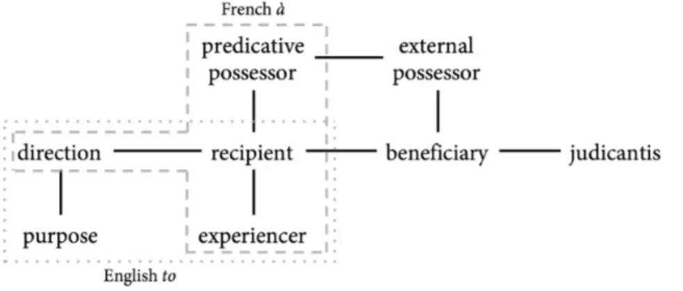
FIGURE 1b Semantic map of dative functions,
with the areas covered by English to and French à (adapted from Haspelmath, 2003: 213, 215)
In order to visualize the meanings of language-specific items, one simply has to map them onto the graph. Figure 1b illustrates how this mapping works by including the boundaries of the English preposition to and the French preposition à: the two items share the meanings ‘direction,’ ‘recipient,’ and ‘experiencer,’ but ‘purpose’ is only expressed by to and ‘predicative possessor’ by
à. Furthermore, one can notice that they cover connected regions of the graph
(see Section 2b).
Proximity maps, on the other hand, are not graphs: the meanings or uses, represented by points, are distributed on a two-dimensional space using multivariate statistical techniques (usually Multi-Dimensional Scaling, MDS in short). The distance between the points of the map is indicative of their (dis)similarity, hence the label ‘proximity map.’ Like classical semantic maps, proximity maps can be construed based on a semantic analysis of cross-linguistic data, but they may also be plotted on the basis of data alone (Narrog & van der Auwera, 2011: 320–321). As such, they are a way to do ‘typology without types.’
2 Polysemy refers to the phenomenon, whereby two or more related meanings are associated
with a single lexical, grammatical or even constructional item. In the literature, the terms ‘multifunctionality’ or ‘polyfunctionality’ are also used to refer to polysemous grammatical items (see, e.g., the use of the term ‘multifunctionality’ by Haspelmath 2003 in the context of semantic maps). For lexical items, François (2008) coined the term ‘colexification’ to refer to “the capacity, for two senses, to be lexified by the same lexeme in synchrony” (François, 2008: 171).
3 FIGURE 1c Spatial model of tense and aspect with Dahl’s prototypes (Croft & Poole, 2008: 26) Figure 1c, for instance, is based on a large dataset of tense-aspect constructions (Dahl, 1985). The points on the map are contexts of occurrence of prototypical tense-aspect clusters (e.g., H = Habitual; S = Habitual Past; O = Progressive; U = Future; V = Perfective), and the distance between any pair of dots reflects the probability that two contexts will be expressed by the same form in the languages of the sample. As can been observed, the points cluster rather well from a semantic point of view, and can subsequently be analyzed along two axes: imperfective–perfective and future–past.
Details about the two different types of maps, their premises, and the generalizations that emerge from each of them will be given in several parts of the paper. The paper is structured as follows. Section 2 discusses the basic principles underpinning the construction of classical semantic maps. Section 3 examines the usefulness of this approach for both typological and language-specific linguistic studies. Section 4 presents the different kind of representation techniques used in the literature for classical semantic maps, and the types of knowledge that these representations capture. Based on a critical evaluation of the classical model, Section 5 introduces the proximity maps, which are based on an alternative plotting method and visualization technique. An overview of the literature on semantic maps is provided in Section 6, and we describe future avenues for the field in Section 7, focusing on the tools that allow an automatic plotting of classical semantic maps based on cross-linguistic polysemy data.
2 | HOW IS A CLASSICAL SEMANTIC MAP BUILT?
In order to describe the steps involved for building a classical semantic map, we take as point of departure Hjelmslev’s (1961: 54) famous example regarding the linguistic expressions of meanings belonging to the semantic field TREE-WOOD -FOREST, as articulated in Haspelmath (2003: 237). Looking at four languages,4
namely Danish, French, German, and Spanish, the lexemes in this semantic field compare as follows:
TABLE 1 Lexemes for TREE/WOOD/FOREST in four languages
Lexical items
Danish French German Spanish
Trӕ
Arbre Baum árbol
Bois Holz
madera
leña
Skov Forêt Wald bosque selva
Table 1 shows that each language lays down its own boundaries at the semantic level (the content-form in Hjelmslev’s terminology). To put it otherwise, one observes a specific partitioning of the semantic domain by language-specific forms. The challenge for the semantic map method is to turn Table 1 into an informative map, which will reflect the regular cross-linguistic relations between the meanings of these language-specific lexical items. From Hjelmslev’s relativism to the kind of universalism postulated by the semantic map model (see Section 3), there are just two steps, which should be taken in the strict following order.
(a) Identifying the meanings (nodes of the map). The individual nodes (or vertices) of a semantic map are inferred from empirical evidence. Meaning identification is based on the analytical primitive principle (Cysouw, 2007, 2010a) According to this, a node N is an analytical primitive, if it cannot be subdivided into two (or more) meanings that are expressed by separate linguistic items in a given language. In practical terms, this means that a new node can be added to the map if and only if there is at least one language with a dedicated linguistic form for this node (Haspelmath, 2003; see further François, 2008). This principle therefore ensures that distinctive meanings will be as
linguistically relevant as possible and will not just rely on linguists’ idiosyncratic
analyses. In Table 2, for instance, in the absence of Spanish a distinction between the meaning WOOD (material) and FIREWOOD would not be justified. It is indeed the
sole language in this table with a specific linguistic form for these two meanings, while Danish, French and German have a single lexical item to express both meanings.
TABLE 2 Partitioning of the TREE–WOOD–FOREST semantic domain
Lexical items
Danish French German Spanish
AN AL YTI CAL PRI M IT IV ES TREE Trӕ
arbre Baum árbol
WOOD (mat.)
bois Holz
madera
FIREWOOD leña
FOREST (small) Skov Wald bosque
FOREST (large) Forêt selva
In accordance with the analytical primitive principle, five nodes can be identified based on the small language sample in Table 1. We use English as metalanguage
5
and label these nodes: TREE, WOOD (material), FIREWOOD, FOREST (small), and FOREST
(large). The semantic map method is neutral as regards the interpretation of these nodes or meanings. Some linguists see them as cognitively salient (Croft, 2001; but see Cristofaro, 2010 for a critique of this position), while other consider them to be merely comparative concepts (Haspelmath, 2010; 2016), specifically created by linguists for the purpose of comparing language specific categorizations in the semantic domain (see Section 7).
It is worth noticing that, when building a semantic map, both the onomasiological and the semasiological approaches can be used independently or combined (de Haan, 2010; Zwarts, 2010b: 124): with a top-down (onomasiological) approach, a given semantic/functional domain is investigated and the relevant linguistic expressions are listed (and subsequently structured) for each language; with a bottom-up (or semasiological) approach, language specific grams, lexemes or constructions and their multiple meanings are the starting point.
Most studies first proceed onomasiologically: they pick a particular domain, identify the core meanings in this domain, and search for the individual forms that express these meanings in different languages. In a second step, the semasiological dimension usually kicks in: one lists in a lexical matrix (Table 3) all the meanings attested for each form of the language sample. In such lexical matrices, if there are two or more √ in the same row, it means that the linguistic form is polysemous, while if there are two or more √ in the same column, the related linguistic forms are translational equivalents.
TABLE 3 Lexical matrix for TREE/WOOD/FOREST in four languages
MEANINGS
TREE (mat.) WOOD FIREWOOD (small) FOREST (large) FOREST
Danish Trӕ √ √ √ – – Skov – – – √ √ French Arbre √ – – – – Bois – √ √ √ (√) Forêt – – – (√) √ German Baum √ – – – – Holz – √ √ – – Wald – – – √ √ Instead of picking one whole domain, other studies choose a single meaning as a pivot of the map. Taking as a point of departure the intra-linguistic onomasiological perspective, these studies first ask what are the words that express the meaning in question in a particular language. In the subsequent semasiological analysis, they list the different meanings of the relevant linguistic items in a language. The final step includes repeating this two-step process in the whole language sample chosen (see François, 2008; Rice & Kabata, 2007; Georgakopoulos et al., 2016). An illustration of the result of such an approach is provided in Figure 2.
6
FIGURE 2 A (partial) semantic map for BREATHE combining both
the onomasiological and the semasiological approach (François, 2008: 185)
This semantic map resembles a language-specific polysemy network, one of the differences being that the pivot (the notion BREATHE in Figure 2) is not similar to
the prototypical meaning (see François, 2008: 181).
(b) Linking the meanings (edges of the graph). In the semantic map model,
the process of linking nodes follows a principal constraint known as the connec-tivity hypothesis: “any relevant language-specific and construction-specific
category should map onto a CONNECTED REGION in conceptual space” (Croft, 2001:
96), “more precisely, a connected subgraph” (Croft & Poole, 2008: 4). As Andrason (2016: 2) puts it, the meanings
“are connected because they arise due to human cognitive mechanisms, being derived by means of metaphor, image-schema process, metonymy, analogy or abduction [… and o]n the other hand, they constitute a temporally sequential chain of predecessor and successors”.
As such, conceptual and historical factors support the connectivity hypothesis. In practical terms, this means that polysemous linguistic items are decisive when plotting a map. Indeed, they are the ones that will be mapped onto two (or more) nodes, and they indicate thereby which nodes should be connected: by virtue of the connectivity hypothesis, they must cover a connected region in the semantic map. Based on the data in Table 2, one can induce the following edges (Figure 3): the meanings TREE and WOOD can be connected, because they are expressed by a
single word in Danish, the polysemous item træ (edge 1); the same applies to the meanings WOOD and FOREST (small), which can be linked because of the French
polysemous item bois (edge 2), and to the meaning FOREST (small) and FOREST
(large), because of the Danish and German lexemes skov and Wald (edge 3).
7
FIGURE 3 A semantic map inferred from the data in Table 2
The boundaries delimited by particular linguistic items in a language are conventionally represented by closed curved lines. For example, the boundaries of the German lexical items Baum, Holz, and Wald are shown in Figure 4. As expected, they do cover strictly connected regions of the map.
FIGURE 4 A semantic map inferred from the data of Table 2, with the German lexemes mapped onto the nodes
A second principle at work when plotting semantic maps is what we call the
economy principle: given three meanings (Meaning1, Meaning2, Meaning3), if the linguistic items expressing Meaning1 and Meaning3 always express Meaning2, there is no need to draw an edge between Meaning1 and Meaning3 (the resulting map will be linear, Meaning1—Meaning2—Meaning3, and not triangular, with all the meanings connected). For example, even if Danish trӕ would allow us to directly connect the nodes FIREWOOD to TREE, and although French bois could lead
to linking FIREWOOD to FOREST (small), a single edge between FIREWOOD and WOOD
(edge 4) is actually enough in order for the connectivity hypothesis to be respected. Then, the only reason to draw an edge between the meanings
FIREWOOD and TREE, or between FIREWOOD and FOREST (small), would be to identify
a language in which these two meanings are expressed by a specific lexeme, which would crucially not express the meaning WOOD (that acts presently as an
intermediate node between these two meanings).
The semantic map in Figure 3 was plotted in a strictly inductive fashion (which is called the “matrix-driven” approach in Zwarts, 2010a: 378–379). In practice, however, one can observe “a combination of deductive semantic analysis and inductive generalizations on a sufficiently large sample of languages” (van der Auwera & Temürcü, 2006: 132). Some semantic map-like networks were even entirely developed following a deductive method (which is called the space-driven approach in Zwarts, 2010a: 379–382): they are either based on extra-linguistic data (e.g., the organization of color chips into a color space according to physical features of hue, saturation, and brightness; e.g., Regier, Kay, & Khetarpal, 2007) or are the product of pre-empirical conceptual analysis (e.g., Lakoff, 1987, on the English preposition over). They can be considered as a good starting point for plotting actual semantic maps, but should
8 be tested against cross-linguistic data in order to assess the empirical validity of their claims regarding the organization of the semantic level.
3 | WHAT ARE THE ADVANTAGES OF
THE SEMANTIC MAP MODEL?
The semantic map model is not a theory of grammar, but as Cysouw (2007) phrased it “a model of attested variation, which might […] be the basis for the formulation of a theory.” It has several significant advantages that make it a useful tool to describe both “language universals and language-specific grammatical knowledge” (Croft, 2003: 133). In what follows, we synthesize its main advantages.
3.1. Advantages of semantic maps as a typological method
A first advantage is that it is neutral with respect to the monosemy/vagueness-polysemy-homonymy distinction (Haspelmath, 2003). A monosemic approach would consider the different meanings of a form as being contextually driven (based on a vague or underspecified meaning); a polysemic account would recognize that different related meanings are associated with each lexical item; a
homonymic position would argue that each meaning of a linguistic item on the
map corresponds to a single form.3 By not taking sides, the semantic map model gives a way out of the problems arising in adopting one of the stances. More specifically, its neutral perspective facilitates cross-linguistic comparison, an area in which the aforementioned approaches have little to offer. The very general meanings identified in monosemic analyses and the more sophisticated (but pertaining to language-specific grammars) networks constructed in studies that favor polysemic analyses, albeit both useful in some contexts, are not well suited for comparing languages (see Haspelmath, 2003: 213–214, 230–232).
An additional advantage stemming from the neutral character of semantic maps is that they can be fruitfully used in various frameworks. Most scholars merely employ them as a tool (a tertium comparationis) for studying cross-linguistic (as well as language specific) patterns of polysemy, while remaining agnostic and refraining from any claim about their cognitive reality or universalism (Cysouw, 2007: 227). Other scholars, on the contrary, . argue that the network of meanings can be envisioned as a universally valid organization of conceptual knowledge across languages, a ‘geography of the human mind,’ as Croft (2001: 139) puts it. Designations such as ‘cognitive map’ (Kortmann, 1997), ‘conceptual space’ (Croft, 2001; 2003), or ‘mental map’ (Anderson, 1986) are representative of this trend. Semantic maps are in this case understood similarly as the ‘networks’ typical of cognitive grammar approaches (e.g., Langacker, 1988; Sandra & Rice, 1995). Yet other scholars are explicitly critical of the position that semantic maps give access to a universal arrangement of different conceptual situations in a speaker's mental representation (Cristofaro, 2010; see
3 We make a distinction here between homonymic interpretations of a map, and the purposeful
integration of homonyms in a single map, which is admittedly a problem since it generates uninformative maps, as discussed by van der Auwera & Temürcü (2006: 133) and van der Auwera, Kehayov, & Vittrant (2009: 297).
9
also Janda, 2009). Despite the disagreements on how far the model can go, semantic maps constitute a suitable model for every approach mentioned.
Furthermore, the meanings or nodes of semantic maps can be of any kind, that is, ‘grammatical,’ ‘lexical’ or ‘constructional’ (see Section 6). Semantic maps can be used for any kind of structured semantic relationships. As a result, any area of the language can be investigated with a single tool, and there is no need to discriminate between the various kinds of meanings, the boundaries of which are not always clear-cur anyway.
Yet another advantage of semantic maps as a typological method is that they are at the same time implicational (Haspelmath, 1997a) and falsifiable (Cysouw, Haspelmath, & Malchukov, 2010: 1). This means that they articulate implicational hypotheses that are deemed to be universally valid as long as they are not falsified, i.e., contradicted by new empirical evidence. For example, based on Figure 2 one can hypothesize that, if a language-specific lexical item expresses both the meaning TREE and the meaning FIREWOOD (like Danish trӕ), then it will
necessarily express the meaning WOOD. If a given language turns out to have a
single form expressing the meanings TREE and FIREWOOD, but not the meaning WOOD, then the map has to be emended4 and new implicational universals can be
formulated.
3.2. Advantages of semantic maps as a semantic method
As shown in Section 2, semantic maps allow one to combine the onomasiological and semasiological perspectives, thus offering a semantically holistic view (see Lehmann, 2004; Geeraerts, 2010: 23; with Gast, 2009: 212–213, specifically about semantic maps). The method proves directly useful both to answer the question of how languages express particular meanings or entire semantic fields (onomasiology) and to chart the different meanings of particular linguistic units in a given language (semasiology). In our example (Tables 1–2, Figure 1), the onomasiological analysis reveals that the meaning WOOD is designated by the
lexical items trӕ (Danish), bois (French), Holz (German), and madera (Spanish). Additionally, it gives intra-linguistic information, in that it indicates, for instance, that bois and forêt in French are near-synonyms for the meaning FOREST
(onomasiological viewpoint). The semasiological analysis, on the other hand, shows that the lexical unit trӕ (Danish) covers three meanings. It also reveals that there are polysemic patterns recurring cross-linguistically, as indicated by the case of the Danish skov and the German Wald covering a similar region of the map. To sum up, with semantic maps, we are able to search for translational equivalents cross-linguistically and designations of a particular meaning intra-linguistically, on the one hand, and for regular and language-specific regular polysemy patterns (Cysouw, 2010b; Perrin, 2010), on the other hand (Table 4).
TABLE 4 The semasiological and onomasiological features of semantic maps
4 The map does not need to be revised, if (a) one is dealing with homonyms, or (b) it can be
shown that this meaning was present in the language at some point in the past, but has been taken over by another form (borrowed or not); see the discussion on Figures 10a–d below.
10
Cross-linguistic Intra-linguistic Onomasiology Translational equivalents near-synonymy Synonymy and
Semasiology Regular polysemy patterns Structured polysemy patterns
Finally, semantic maps have proven to be an efficient tool in historical linguistics, and especially in grammaticalization studies (e.g., Narrog & van der Auwera, 2011). Synchronic semantic maps can indeed be interpreted diachronically, as they make prediction about the meanings to which a given form could extend, and a proper methodology has been elaborated for diachronic semantic maps, which explicitly visualize the attested pathways of evolution. This approach is discussed in Section 4.
4 | LINKING MEANINGS WITH SEMANTIC MAPS:
TYPES OF RELATIONSHIPS, DIACHRONY, AND FREQUENCY
The semantic maps discussed in Sections 2 and 3 are classical semantic maps (also known as ‘traditional’ in Malchukov, 2010, ‘first generation’ in Sansò, 2010, ‘implicational’ in Wächli, 2010, or ‘connectivity maps’ in van der Auwera, 2013). They usually take the form of two-dimensional graphs, with nodes (technically called ‘vertices’) connected by lines (technically called ‘edges’).
FIGURE 5 Semantic map of dative functions (adapted from Haspelmath, 2003: 213)
In the simplest form of classical semantic maps, the nodes are generally displayed with (or as) labels referring to a meaning, their precise position does not matter, and the length of the lines between nodes is irrelevant (Haspelmath, 2003: 216). The graph structure is the only aspect that really matters —formally speaking classical semantic maps are undirected graphs—, which means that the similarity between two meanings depends on the number of intervening nodes (van der Auwera, 2013: 156). Thus, in Figure 1a, which we repeat here as Figure 5 for convenience, the distance between PURPOSE and EXPERIENCER is greater than
the distance between PURPOSE and DIRECTION, because one has to pass two nodes
to reach the former and none to reach the latter. The meanings PURPOSE and DIRECTION can thereby be inferred to be semantically closer than PURPOSE and EXPERIENCER. As stated above, the precise position of the node on the plane is not
meaningful in this mode of representation. In Figure 5, for instance, the spatial distance between PURPOSE and EXPERIENCER is (more or less) the same as the one
11
between PURPOSE and DIRECTION, but this only reflects an arbitrary positioning of
the nodes and cannot be taken as evidence for proximity in meaning: the number of edges between nodes is the only thing that matters.
Several visualization techniques have been used in order to expand this basic type of representation and to capture graphically more information while remaining within the classical semantic maps model. In the literature, these techniques apply to three main kinds of information: (a) information about the types of relationships between the meanings; (b) diachronic information, and (c) information about the frequency of polysemy patterns.
(a) In order to visualize different types of relationships between meanings, van der Auwera and Plungian (1998) represented meanings with elementary set-theoretical means: the inclusion of one oval into another indicates a hyper-/hyponymic relationship, while connecting two ovals with a line points to a metonymical (or metaphorical) link (van der Auwera, 2013: 161–162).
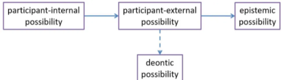
FIGURE 6 A mini-map of modal possibility
(van der Auwera & Plungian, 1998: 87, Fig. 1)
In Figure 6, DEONTIC POSSIBILITY (e.g., “as far as I’m concerned, you may go to the
party tonight”) is defined as a subtype (hyponym) of PARTICIPANT-EXTERNAL POSSIBILITY (e.g., “you may take the bus in front of the train station”), while PARTICIPANT-EXTERNAL POSSIBILITY and EPISTEMIC POSSIBILITY (e.g., “he may be at the
office right now”) are seen as metonymically related. As observed by Zwarts (2010a: 384–385), these types of semantic relationships could be represented as well by different types of lines. Figure 7 is a (visually less expressive) translation of Figure 6. Adhering to this alternative representational mode a dashed line is used for the hyper-/hyponymic relationship, while a solid line is used for the metonymic (or metaphorical) links. Note that this visualization technique is not ideal for unbalanced semantic relations, like the one between a generic term and a more specific one, since one loses information about which node is the hypernym and which node is the hyponym.
FIGURE 7 A mini-map of modal possibility (adapted from Fig. 6)
12
(b) The example of Figure 6 displays another striking feature: the nodes are not connected by mere lines, but by arrows. This graphic device is used to integrate diachronic information about directionalities of change. Adding information about diachrony in a map is known as ‘dynamicizing’ a map (Narrog & van der Auwera, 2011: 323–327). Drawing from the terminology of graph theory, we define a dynamic semantic map (a dysemap) as a set of vertices connected by edges that are allocated a direction. These directed edges are called ‘arcs’ and can represent different types of semantic shifts, such as ‘semantic generalization’ or ‘specialization’ in the case of hyper-/hyponymic relationships, or ‘semantic extension’ when metaphorical and metonymical processes are involved (van der Auwera, 2013; Luraghi, 2014). Ideally, the dysemap would behave like a common directed graph (digraph in graph theory terminology), in that one single direction would be imposed on every edge (cf. Figures 8a–b), which is often the case for the semantic maps about grammaticalization pathways (that are largely unidirectional). FIGURE 8a A simple dysemap (Narrog, 2010: 234) FIGURE 8b A simple digraph (Balakrishnan & Ranganathan, 2012: 40)
However, due to lack of data, it can happen that no directionality can be established between some vertices of a dysemap (in this respect, see the overlooked connections discussed in Narrog, 2010: 242, and Figure 9 below), or that, due to controversial directionalities (e.g., Narrog, 2010) or attested bi-directionalities (e.g., van der Auwera & Plungian, 1998: 100, 111; Luraghi, 2001: 50; van der Auwera, Kehayov, & Vittrant, 2009: Maps 6 and 10), a double-headed arc connects a pair of vertices. FIGURE 9 A semantic map for conjunction and related functions (Haspelmath 2004: 21), with added directionalities (Narrog & van der Auwera, 2011: 326) Even if only a small portion of semantic map research has tried to integrate the diachronic dimension so far (see Section 6), these efforts turn out to be crucial from a methodological point of view (van der Auwera, 2008; van der Auwera, 2013: 164–167), since they allow one to explain exceptions to the connectivity hypothesis (Section 2). Let’s consider an abstract example in order to illustrate
13
this point. In the hypothetical scenario of the synchronic semantic map of Figure 10a, in which meaning A is connected to both meaning B and C, imagine the case of a linguistic item expressing both MEANING B and MEANING C (shaded in
Figure 10a), but not MEANING A. One would have to posit an edge between MEANING B and MEANING C, making the map vacuous (Figure 10b) and much less
informative, since all the meanings are connected. A dysemap approach of the same meanings, however, will allow formulating the hypothesis that both the
MEANING B and MEANING C attested in synchrony for a linguistic item derive from
an earlier meaning A (and not to draw an edge between those meanings, at least provisionally; cf. Figure 10c). Consequently, the strictly inductive, matrix-driven, approach cannot be straightforwardly applied with the dysemaps. FIGURE 10a A simple semantic map FIGURE 10b A vacuous semantic map FIGURE 10c A simple dysemap FIGURE 10d An oriented dysemap
Another advantage of the dysemaps is that, even if all the meanings are connected (Figure 10d), they allow generalizations that would not be possible with vacuous synchronic semantic map (like Figure 10b; cf. Narrog, 2010: 234– 235). Figure 10d, for example, illustrates the fact that MEANING C is a semantic
extension of either MEANING A or B, but makes the prediction that the opposite
semantic shift is not possible.
(c) Besides the representation of different types of semantic relationships and the visualization of dynamic links between nodes, classical semantic maps can also integrate information about the frequency of polysemy patterns. As stressed by Cysouw (2007: 232), in traditional semantic maps, “the boundary between attested and unattested is given a very high prominence,” since the unique attestation of a polysemy pattern will be represented on the map exactly as a very common one, namely with a simple edge between two nodes (see further Croft & Poole, 2008). In order to address this issue, information about the frequency of polysemy patterns can be visualized in three different ways, using the length of the edges (called ‘proximity’ in van der Auwera, 2013: 156–157), the types of the edges, or the thickness of the edges. FIGURE 11 One-dimensional semantic map in which the length of the edges is meaningful (Nikitina, 2009: 1116)
14
Figure 11 illustrates the length strategy: the difference in length of the edges between the nodes captures the cross-linguistic tendency for GOALS and PLACES to
receive identical encoding, which is not so robust for PLACES and SOURCES (see
Nikitina, 2009: 1116–1117). Semantically, the semantic roles GOAL and PLACE will
then be understood as more tied than PLACE and SOURCE.
In Figure 12, one observes different types of edges —solid lines, square dotted lines, round dotted lines, and long dashed lines— in order to represent different degrees of dependency of one meaning to another (Narrog & Ito, 2007: 281–282). The solid lines, for example, indicate that a meaning depends on another one by more than 90 %, with at least ten morphemes for which both meanings are available in a dataset of 200 languages; the square dotted lines, on the other hand, allow visualizing the dependency between three meanings (and not two), available in at least five morphemes (CLAUSAL COORDINATION – NP-COORDINATION – COMITATIVE is an example of such a dependency). As can be
observed, including information about the frequency of different kinds of polysemy patterns leads to the multiplication of the number of edges between nodes.
FIGURE 12 Visualizing different types of frequency
in the semantic map of the Comitative-Instrumental domain (Narrog & Ito, 2007: 283)
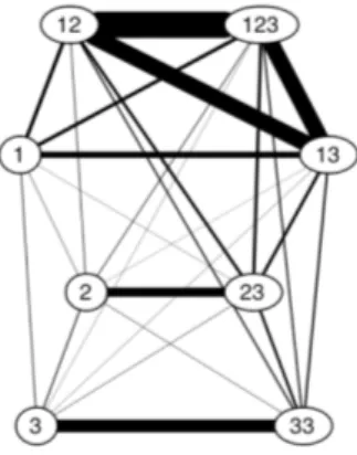
In his map of person marking, Cysouw (2007) provides a third solution for representing frequency, by using weighted edges whose thickness is proportional to the frequency of occurrence of the meaning pairs (see also Forker, 2016: 87). FIGURE 13a A simple semantic map FIGURE 13b A weighted semantic map
15
of person marking of person marking
(Cysouw, 2007: 231, 233)
In the maps of Figures 13a and 13b, the numbers correspond to different primitives, which reflects the linguistic diversity of person marking in the languages of the world. The weighted edges in Figure 13b capture the frequencies of each polysemy pattern. The difference in thickness between the edge that connects node 1 (SPEAKER) to 12 (DUAL INCLUSIVE) and node 12 (DUAL INCLUSIVE) to 123 (PLURAL INCLUSIVE) represents the difference in frequency of
colexification of the two pairs of primitives across languages (see Cysouw, 2007: 232–234). Not only is this kind of weighted classical semantic map much more informative than simple semantic maps, but it also allows one to simplify the map for the sake of generalizations, based on a principled criterion, namely focusing on the more frequent polysemy patterns (see Malchukov, 2010: 177 about data reduction).
The comparison between Figure 13a and 13b further reveals that the two-dimensional semantic maps, which are almost unanimously preferred5 —since they are easier to represent and read on paper (see Haspelmath, 2003: 218; Narrog & Ito, 2007: 273)—, can be hard to interpret when nodes are densely interconnected and edges cross (technically called ‘non-planar graphs’). In this case, the readability of three-dimensional like semantic maps such as Figure 13b is assuredly better.
Strongly connected maps, i.e., maps in which some nodes are connected to many other nodes, can also be difficult to read and interpret. To avoid this state of affairs, which is a frequent and notable problem when studying the sema-siology of a few lexical items in a given semantic field, the related meanings can also be visualized as neighboring meanings, albeit without connecting lines. In Georgakopoulos et al. (2016) visualizations of this type were possible using a semi-automatic process, which included both automatic and manual arrangements of meanings. In this case, the constraint is to arrange the meanings in such a way that it is possible to encircle contingent areas for all individual lexemes.
5 See however the attempts to map in three dimensions of van der Auwera & Van Alsenoy
16
FIGURE 14 The semantic space of EARTH/ SOIL lexemes in Classical Greek
(Georgakopoulos et al., 2016: 440)
The map is valid as long as we are able to draw a closed curved line around all the meanings expressed by the lexemes, as is the case with Figure 14, which shows how Classical Greek lays down its own boundaries in the EARTH/SOIL
domain. The same principle is applied in Tenser (2016: 225–235) when studying the influence of Russian and Polish on the case representation system of Romani.
5 | PROBLEMS WITH CLASSICAL SEMANTIC MAPS
AND ALTERNATIVE MODELS
Starting with Cysouw (2001), the classical semantic map model discussed so far has been questioned and criticized for three main reasons.6 First, “the precise predictions that can be formulated on the basis of [an] implicational map are unclear,” because it “predicts much more than is actually found” (Cysouw, 2001: 609–610). To put it otherwise, the model is too strong for the data on which it is based: it overgenerates constellations, favoring high coverage over high accuracy (Cysouw, 2007: 234–235; Croft & Poole, 2008: 6; Malchukov, 2010: 176). This point is easily illustrated based on the map of Figure 16a below. Theoretically, there are 105 different possibilities for mapping a linguistic form, whereas Haspelmath (2003: 76) states that only 39 different kinds of mapping are actually found in his dataset. Second, “as the amount of data increases, vacuous maps become more and more widespread since frequent, rare and exceptional patterns will all be represented on the map” (Malchukov, 2010: 176). Third, classical semantic maps could not be generated automatically at the time and were considered “not mathematically well-defined or computationally tractable, making it impossible to use with large and highly variable crosslinguistic datasets” (Croft & Poole, 2008: 1).
6 We focus here exclusively on issues that have not been addressed in the previous sections. The
issues connected to the visualization of frequency patterns, for instance, are dealt with in Section 4 (see also the discussion in Malchukov, 2010: 176–177).
17
In order to cope with these issues, statistical scaling techniques — especially MDS—, which are particularly efficient in dealing with big data, were introduced by several scholars as alternative or complementary visualization methods. MDS is basically a means of visualizing spatially similarities and dissimilarities between pairs of items. To paraphrase Cysouw (2007: 236, 241), the general idea behind the mathematical analysis is that the distance between two meanings in a two-dimensional Euclidian plane is iconic to the chance of co-occurrence of these meanings within a single linguistic expression (Schiffman, Reynolds, & Young, 1981; Groenen & van de Velden, 2005: 1280; Croft & Poole, 2008). Maps of this type are called, ‘similarity’ (Malchukov, 2010: 176), ‘second generation’ (Sansò, 2010), ‘statistical’ (Wälchli, 2010), ‘probabilistic’ (Wälchli & Cysouw, 2012), or ‘proximity’ maps (van der Auwera, 2013). FIGURE 15a MDS analysis of Haspelmath’s 1997a data on indefinite pronouns (Croft & Poole, 2008: 15) FIGURE 15b Cutting lines for Romanian indefinite pronouns (Croft & Poole, 2008:16)
Figure 15a, taken from Croft and Poole (2008), exemplifies this visualization technique. It is based on Haspelmath’s (1997a) data used for the study of the semantics of indefinite pronouns. It tells us, among other things, that an indefinite expression occurs more frequently across languages with both the functions SPECIFIC, KNOWN TO THE SPEAKER (spec.know) and SPECIFIC, UNKNOWN TO THE SPEAKER (spec.unkn) than it does with both the function SPECIFIC, KNOWN TO THE SPEAKER (spec.know) and IRREALIS, NON SPECIFIC (irr.nonsp). In this case, the
positioning of the various meanings on the two-dimensional plane is not the only product of MDS. An important aspect here is the addition of cutting lines, which correspond to the boundaries of the language-specific forms: as shown in Figure 15b for Romanian indefinite pronouns, these cutting lines fulfill the same function as the closed curved lines in the classical semantic map model (see Figures 1a, 4, and 14) showing which form expresses which function(s).
However different the classical semantic maps approach and the MDS procedure may seem, they can be thought of as compatible and complementary (van der Auwera, 2008, 2013; Mauri, 2010). In fact, they are able to represent the same structure of the conceptual space when visualizing the same data (Croft & Poole, 2008: 19). This point can be illustrated by comparing Figure 16a, namely Haspelmath’s (1997a) original semantic map of the indefinite pronouns functions, with Figure 16b, the MDS analysis by Croft and Poole (2008) of the
18
same data (cf. Figure 15a), with the superimposed graph structure of the classical semantic map. The curved horse-shoe shape of the arrangement of the points in the two-dimensional MDS visualization is typical, and explained by the fact that a single cutting line needs to be able to delimitate the language specific categories in the Euclidian plane (cf. Figure 15b, with Croft & Poole, 2008: 17– 18). FIGURE 16a Haspelmath’s (1997a: 4) original semantic map of the indefinite pronouns functions Figure 16b MDS analysis of Haspelmath’s 1997a data with the superimposed graph structure (Croft & Poole, 2008: 17, Fig. 6) However, the input for such proximity maps is often of a different nature. In most of the cases, proximity maps are not constructed on the basis of a lexical matrix with identified meanings that result from a preliminary analysis of the crosslinguistic material (like in the example just discussed). Rather, more frequently they are compiled from responses to linguistic (e.g., Croft and Poole, 2008: 22–31, who rely on Dahl’s 1985 database) or non-linguistic materials (see Levinson et al., 2003: 503–513; see also Majid, Boster, & Bowerman, 2008 for a similar semantic map-like approach, which uses correspondence analysis), or directly plotted based on parallel corpora (Wälchli, 2010; 2016; Wälchli & Cysouw, 2012). In this case, what is represented via MDS, i.e., the analytical primitives, is the distribution of the actual coding means in context (and not meanings). This is a method for doing ‘typology without types’ (Wälchli, 2010: 347; Wälchli & Cysouw, 2012: 702–703).
19 FIGURE 17 MDS visualization of the French local phrase markers in the Gospel of Mark (Wälchli, 2010: 348) Figure 17 nicely illustrates this method. The position of the points corresponds to the distribution of 190 motion event clauses from translations of the Gospel of Mark (153 languages from all continents) based on the (dis)similarity between
the local phrase markers (adposition and/or case) used in each clause (i.e., in each specific context). The colors and shapes of the points, on the other hand, correspond to the mapping of the French coding means. Such a map must therefore be analyzed in two different ways. First, one has to explain the clustering of the points (in this case, the motion event clauses). The parameters are not given, but the result of the statistical analysis (Hamming distance as a distance measure, in this case): dimension 1 and dimension 2 need to be interpreted. Having studied the mapping of the local phrase markers on these points, Wälchli (2010: 347–349) concludes that dimension 1 corresponds to
SEMANTIC ROLES variation (as it distinguishes neatly SOURCES and GOALS), while
dimension 2 likely represents the combination of ANIMACY and LOCALIZATION
(i.e., movement ‘to,’ ‘unto,’ ‘into’).7 Figure 17 displays the result of this analysis with labels for the main clusters: COMPANION, (IN)ANIMATE GOAL, PATH, and SOURCE.
In a second step, the mapping of the language-specific local phrase markers can be analyzed. To take a single example, one can observe in Figure 17 some uses of the French preposition de (‘from’) in goal oriented motion events. These outliers can be explained by the occurrence of this preposition in the valency pattern of s’approcher de X ‘to approach X’ and in the compound preposition de
l’autre côté ‘at/to the other side’ (Wälchli, 2010: 147).
As stressed by Grossman and Polis (2012: 185) and exemplified by the discussion of Figure 17, the main difference between the classical semantic maps model and the distance-based representations is that the former is an explanans —being the result of crosslinguistic investigations and implying a semantic analysis that precedes the construction of the map—while the latter is an
7 The MDS visualization tries to show as much as possible of the actual distances, but needs to
convert the many dimensions of the dataset into a two-dimensional plane. Consequently, the dimensions can turn out to be difficult to interpret, and the emerging picture can turn out to be hard to read (cf. Cysouw, 2007: 237).
20
explanandum (cf. van der Auwera, 2008): the maps are plotted directly based on
the data (which are constructed and not given, see Wälchli & Cysouw, 2012) and these represent the point of departure of the analysis. Consequently, distance-based maps are not implicational and cannot be used to constraint the data (Malchukov, 2010: 177)
It should be stressed that the MDS method has been criticized because it cannot take into account diachronic information, if available (van der Auwera, 2008, 2013; Narrog, 2010). For example, there is no way to infer any directionality from Figure 15a. The classical ‘connectivity’ maps on the other hand predict that “a category can acquire a new function only if that function is adjacent on the semantic map to some function that the category already covers” (Haspelmath, 1997a: 129). The arrangement of the same meanings in Figure 16a indeed allows us to predict that, if an originally FREE CHOICE marker extends to
also cover the QUESTION/CONDITIONAL function, then that marker should first
extend to cover the COMPARATIVE function. Thus, interpreted diachronically,
classical semantic maps make predictions similar to the synchronic (implicational) maps. Up until recently (see Section 6), however, the statistical approach was the only way to handle large typological datasets and to generate automatically maps for studying cross-linguistic diversity.
6 | SURVEY OF THE LITERATURE ON SEMANTIC MAPS
Any type of meaning can be integrated in semantic maps, such as the meanings of grammatical morphemes, of entire constructions, or of lexical items. From a methodological point of view, there is no need to distinguish between them, since the method can be used for any kind of structured semantic information.
Grammatical semantic maps cover a wide range of linguistic phenomena (cf. van der Auwera & Temürcü, 2006: 132; Cysouw, Haspelmath, & Malchukov, 2010a; Narrog & van der Auwera, 2011): tense and aspect (Anderson, 1982),
reflexives and middles (Kemmer, 1993), indefinite pronouns (Haspelmath, 1997a), impersonal constructions (Malchukov & Ogawa, 2011; Siewierska & Papastathi,
2011; van der Auwera, Gast, & Vanderbiesen, 2012; Gast & van der Auwera, 2013), modality (van der Auwera & Plungian, 1998; van der Auwera et al., 2009; Simon-Vandenberge & Aijmer, 2007: ch. 10; Boye, 2010), temporal markers (Haspelmath, 1997b), encoding of core arguments (Croft, 2001: 134–147),
semantic roles (Luraghi, 2001; Haspelmath, 2003; Clancy, 2006; Narrog & Ito,
2007; Rice & Kabata, 2007; Malchukov & Narrog, 2009; Luján, 2010; Malchukov, 2010; Wälchli, 2010; Grossman & Polis, 2012; Hartmann, Haspelmath, & Cysouw, 2014; Luraghi, 2014; Mohammadirad & Rasekh-Mahand, 2017), partitive
constructions (Koptjevskaja-Tamm, 2008), the DO/GIVE co-expression (Gil, 2017),
transfer of possession constructions (Collins, 2015), coordination (Haspelmath,
2004: 20–24; Mauri, 2010), complementation (Matras, 2004), adversatives (Malchukov, 2004), intransitive predication (Stassen, 1997), secondary
predication (van der Auwera & Malchukov, 2005; Verkerk, 2009), person-marking (Cysouw, 2007), imperative-hortatives (van der Auwera, Dobrushina, &
Goussev, 2003) negative existentials (Veselinova, 2013), negative polarity items (Hoekstra, 2014), intensifying particles (Forker, 2015), additives (Forker, 2016).
As can be observed, many of the above grammatical semantic maps describe cross-linguistic polysemies of particular constructions rather than of
21
isolated grammatical morphemes. Maps of this type allow one to capture which construction maps onto which category in a given language (see, e.g., Croft, 2001: ch. 2.4). Consider, for example, the semantic map in Figure 18 for depictive adjectival constructions proposed by van der Auwera and Malchukov (2005). FIGURE 18 Semantic map of depictive adjectivals (van der Auwera & Malchukov, 2005: 407) All the constructions visualized in the map belong to the same semantic domain. In compliance with the premises of the semantic map model, (a) the arran-gement of the different types of predication in the graph —namely PRED
(ica-tives), DEP(ictives), COMPL(ementatives), APP(ositives), RESTR(ictives)— reflects
the degree of (dis)similarity among these types; and, (b) certain implicational hypotheses are possible. The map predicts that, if a language uses the same strategy for depictives and restrictives, then it will necessarily use the same strategy for appositives. An example of a language that uses the same adjectival strategy for all three types is English (ex. 1–3) (van der Auwera & Malchukov, 2005). (1) Depictive: George left the party angry (2) Appositive: My father, angry as always, left the party. (3) Restrictive (attributive): The angry young men left the party. In fact, in English all five types receive identical encoding (ex. 4–5). (4) Complementative: I consider John intelligent (5) Predicative: George was angry However, the different types of constructions yield many different permutations. In Russian, for instance, the instrumental forms of the adjective do not distinguish between depictives, predicatives, and complementatives, but they exclude appositives and restrictives (van der Auwera & Malchukov, 2005: 409).
In addition to grammatical and constructional maps, recent research has shown that the semantic map model can fruitfully be extended to lexical items. The starting point of this ‘lexical turn’ can be traced back to François’ (2008) seminal paper, which, building on Haspelmath (2003), provides a blueprint for constructing lexical semantic maps (see Majid et al., 2007 for an early account; cf. Koch, 2001 for an approach similar to semantic maps). François uses semantic atoms or meanings of lexical items in context in order to analyze cross-linguistic patterns of colexification. Other studies that followed focused on polysemic patterns shared by diverse notions in different domains, such as quality expressions (Perrin, 2010; cf. Rakhilina, 2015; Ryzhova & Obiedkov, 2017), notions belonging to the motion domain (Wälchli & Cysouw, 2012) or to the
22
domain of perception (Wälchli, 2016), the notion of emptiness (Rakhilina & Reznikova, 2014; 2016), temperature terms (Koptjevskaja-Tamm, 2015: 17; Liljegren & Haider, 2015: 469; Perrin, 2015), natural and spatial features (Georgakopoulos et al., 2016; Youn et al., 2016), and visual direction (Rakhilina, Vyrenkova, & Plungian, 2017).
It is fair to say that the different types of maps have not received equal attention in the literature. Rather, there is a strong bias towards studies describing cross-linguistic polysemies of grammatical morphemes and constructions. They have occupied a central role within the semantic maps tradition for at least two reasons. First, their study is often considered by linguists to be more interesting and prestigious than the study of the lexicon (Haspelmath, 2003: 211), and consequently data about grammatical functions are more easily collected in the literature than data about polysemic lexical items. Second, the general tendency in the typology was to regard the lexicon as “exuberant and idiosyncratic” (François, 2008: 164). As a result, the lexical domain has generally been neglected, despite the fact that it has always been central for the arguments about cross-linguistic variation at the semantic level.
A common denominator to most of the studies listed above is their synchronic orientation. While it has been claimed that “the best synchronic semantic map is a diachronic one” (van der Auwera, 2008: 43; cf. Section 4 here, with Wälchli & Cysouw, 2012: 703–705), the big bulk of research has been adopting a synchronic perspective, and the limited research that has added the diachronic dimension has focused almost exclusively on the grammatical domain (Lichtenberk, 1991; van der Auwera & Plungian, 1998; Narrog, 2010; Luján, 2010; Eckhoff, 2011; Luraghi, 2014). For lexical typology, semantic maps have been conceptualized explicitly as “a strictly synchronous device,” a stance justified by the complexity of the historical relations between lexical meanings (Rakhilina & Reznikova, 2016: 113; but see Viberg’s 1984 modality hierarchy, which can be seen as a forerunner of lexical diachronic semantic maps). On the other hand, one can notice that the scope of constructional maps has been expanded in order to include the diachronic dimension (Fried, 2007; 2009; Traugott, 2016). Traugott (2016) shows how semantic maps can be used to inform diachronic constructional analyses. For these diachronic constructional maps to work, she argues that two levels are needed: a macro-level, which “represent[s] relationships between abstract, conceptual schemas linked to underspecified form” and a micro-level, “which models relationships among specific micro-constructions” (Traugott, 2016; see also Croft, 2001). These two levels correspond to two kinds of maps each operating at a different level of abstraction: the schema-construction maps and the micro-construction maps, respectively. In incorporating directionality of change, each type makes different generalizations: the former captures tendencies and the latter language-specific paths of change (Traugott, 2016). Figure 19 presents a language-specific path of change in English modals of comparison. Through constructionalization rather extends from the uses ‘instead’ and ‘sooner’ (the [F Adv-er] on the map) to the modal use ‘’d rather’ [F Aux-Adv-er] (a development from non-volitive to volitive; cf. Narrog, 2012). The Figure also captures the association of the RATHER
micro-construction with two larger schema-constructions, the modal schema construction (MODAL.SCXN) and the biclausal comparative schema construction (BCOMP.SCxn), the latter of which is placed outside the modal domain.
23
FIGURE 19 Development of the micro-construction RATHER modeled as a MCM
(Traugott, 2016: 120)
7 | ISSUES, CHALLENGES, AND AVENUES
FOR FUTURE RESEARCH
The great variety of linguistic domains to which the classical semantic map model has been applied highlights its efficiency in capturing regular patterns of semantic structure and cross-linguistic similarities of form-meaning correspondence. In this concluding section, we point out some pending issues, challenges, and promising avenues for future research as regards (1) data collection, (2) the connectivity hypothesis, (3) automatic plotting, and (4) visualization techniques.
7.1. Data collection
One major issue for the semantic map model, which is a recurrent concern in language typology as a whole, is the choice of a good language sample that will allow for valid cross-linguistic generalizations. Haspelmath (2003: 217) argues that a dozen of genealogically unrelated languages usually suffice to arrive at a certain degree of generalization. However, restricting typological research to only a few languages could result in overlooking interesting (even if infrequent) connections between meanings (Narrog & Ito, 2007: 276) or in missing linguistic or culture associations that are specific to geographical regions or areas. Narrog and Ito (2007: 276) suggest that the greater the size of the language sample, the greater the likelihood that the map will be accurate and capture (statistical) universals.8 One important future area of research for the semantic map method would then be to construct and test various areally and genealogically stratified samples (on the language sampling method, see Rijkhoff & Bakker, 1998;
8 In order to construct their map for the COMITATIVE-INSTRUMENTAL area, they relied on a sample of
24
Miestamo, Bakker, & Arppe, 2016, among others; cf. Bickel, 2015 for a caveat on representative samples). One question that will necessarily arise is whether lexical semantic maps should follow the same principles as grammatical semantic maps. In this respect, Rakhilina and Reznikova (2016: 101–102) highlight the fact that some of the restrictions of grammatical typology do not apply to lexical typology. For example, related languages can provide reliable information just as genealogically diverse ones do. Furthermore, despite the increasing availability of resources (such as the Database of Cross-Linguistic
Colexifications [http://clics.lingpy.org], see List et al., 2014), the primary material
for lexico-typological studies is not always sufficient, a factor that may impede large-scale studies. This is one of the main reasons why the number of languages of a typical lexico-typological study ranges from 10 to 50 (see Koptjevskaja-Tamm, Rakhilina, & Vanhove, 2015: 436; cf. Wälchli, 2010; Wälchli & Cysouw, 2012; Östling, 2016, which relied on larger samples thanks to the availability of resources, viz. massively parallel texts).
Besides the quantity of data, the accuracy of a semantic map also depends heavily on the quality of the collected crosslinguistic material, which is best ensured by identifying comparable phenomena across languages. As to what counts as meaning, comparability is reached if the same definition is used, a definition that should ideally be purely descriptive and theory-neutral (see François, 2008: 170; Koptjevskaja-Tamm, 2016: 5). In this respect, the meanings of a map can be seen as comparative concepts (Haspelmath, 2010; see the special issue of Linguistic Typology 20/2 [2016] devoted to this topic), which have to be universally applicable and can be defined based on universal conceptual-semantic concepts, general formal concepts, and other comparative concepts.9
Yet two questions remain to be explored more thoroughly as regards data quality: on the one hand, the level of granularity of the meanings integrated in a semantic map, and on the other hand, the mapping of language-specific forms onto these meanings.
The construction of a semantic map is indeed affected by decisions on the degree of resolution of the semantic distinctions (see Wälchli, 2010: 335). A map of higher resolution means that the analytical primitives used as a basis for plotting it are fine-grained, which leads to more detailed and accurate maps.10 A map of lower resolution helps unravel general tendencies, but will probably fail to capture more infrequent patterns (which however is not always considered as a problem; see François, 2008: 163–164). While it is desirable to combine large crosslinguistic databases and a meticulous semasiological analysis of the selected linguistic items, thus obtaining a higher resolution, this is difficult to put into practice. Furthermore, despite some suggestions for visualizing hyper- and hyponymic relationships (see the discussion of Figure 6 above), the systematic integration of meanings of different degrees of generality within a single semantic map is still to be investigated.
9 For example, a definition of a ‘future tense’ as “[…] a grammatical marker associated with the
verb that has future time reference as one prominent meaning” is based on the conceptual-semantic concept ‘future time reference’ and the comparative concepts ‘verb’ and ‘grammatical marker’ (Haspelmath, 2010: 671).
10 See in this respect Wälchli and Cysouw’s (2012: 680) criticism: “[i]n implicational maps there
are a small number of idealized functions that do not take into account the large amount of domain internal diversity of general abstract labels.”
25
As regards the mapping of language specific forms onto the map, a recurring challenge for the method is that it often attributes meanings to the grammatical or lexical items themselves, despite the fact that we are usually dealing with contextual meanings that are only available for this form in specific constructions (cf. Grossman & Polis, 2012: 197). As Andrason (2016: 7) puts it, “[a] form that is represented by means of semantic maps is typically studied in isolation from the language in which it exists and in which it has been developing. (…) The lack of information concerning environmental factors is particularly suspicious (…).” A solution for integrating information about the construction-specific meanings of the forms that are mapped is yet to be found.
7.2. The connectivity hypothesis
Another pending issue for the semantic map approach is how to account for violations of the connectivity hypothesis (Section 2). These violations can result from three main types of phenomena (e.g., van der Auwera, 2013: 161–162): homonymy, diachrony, and language contact situations.
• Homonyms do not have to cover a connected region of a semantic map. Formal identity does not lead to semantic connectivity in cases such as
lie1 ‘speak falsely’ and lie2 ‘be positioned horizontally’ (van der Auwera, 2013).
• As discussed in Section 4b, dynamicized semantic maps, given their capacity to integrate the diachronic dimension, make it possible to explain the lack of connectedness between the meanings of a given linguistic forms in synchrony if (and only if) these meanings derive from a common ‘ancestor,’ namely a meaning previously expressed by the same form. • In language contact situations, two types of exceptions to the connectivity
hypothesis have been noticed in the literature. First, several scholars observed that areal factors possibly lead to the extension of the meaning of a linguistic form in a given language based on the meaning of a similar expression in a (prestigious) neighboring language (e.g., van der Auwera et al., 2009). This phenomenon, known as ‘polysemy copying,’ has been studied within the classical semantic map method and described with the labels ‘semantic map harmony’ (Tenser, 2008; 2016; see also Matras, 2009: 263–264) and ‘semantic map assimilation’ (Gast & van der Auwera, 2012). Second, in a study about adpositions borrowing between Greek and Coptic, Grossman and Polis (2017) showed that the polysemy network of the adpositions in the donor language is not borrowed as a whole; rather, only some of its meanings are borrowed, which are not necessarily connected on the map.
The clear identification of such exceptions is crucial for the semantic map method, as they directly bear on the automatic inference of semantic maps based on polysemy matrices (see Table 3).
26
As already noted by Narrog and Ito (2007: 280), “ideally (…) it should be possible to generate semantic maps automatically on the basis of a given set of data.” Indeed, it is practically impossible to handle large-scale crosslinguistic datasets manually. However, as noted by Croft and Poole (2008: 7) it was at the time “not clear whether the semantic map model can be automated in a computationally tractable algorithm.” Finding the minimum number of links between nodes for a set of crosslinguistic data is akin to the “traveling salesman problem,” which is known to be NP-hard.11 This potential intractability was considered to be a significant problem for the use of graph-based semantic maps in typology and led to the use of MDS (and similar techniques) for representing similarity between nodes (Section 5).
This state of affairs recently changed, when Regier, Khetarpal, and Majid (2013) showed that the semantic map inference problem is “formally identical to another problem that superficially appears unrelated: inferring a social network from outbreaks of disease in a population” (Regier et al., 2013: 91). This similar inference problem was shown to be indeed computationally intractable, but it was found that “an efficient algorithm exists that approximates the optimal solution nearly as well as is theoretically possible” (Angluin, Aspnes, & Reyzin, 2010). Having tested the algorithm on the crosslinguistic data of Haspelmath (1997a) and Levinson et al. (2003), Regier et al. (2013) concluded that the approximations produced by the algorithm are of high quality, which means that they produce equal or better results than the manually plotted maps. Hence, the graph structure of classical semantic maps can be quite straightforwardly inferred using such an algorithm.
However, very many questions remain to be explored in this highly promising domain. For instance, the algorithm of Regier et al. (2013) produces unweighted and undirected graphs: the automatic addition of weighted edges based on the crosslinguistic frequency of polysemy patterns and the inference of oriented edges based on diachronic information is shown to be both straightforward and highly informative in Georgakopoulos and Polis (2017). Besides, the problem of network inference is a very active research area (especially in biology, where network inference is used for uncovering causal relationships between genotype and phenotype) and the number of available algorithms has grown tremendously during the last decades (e.g., Siegenthaler & Gunawan, 2014). Such algorithms should be tested on large-scale cross-linguistic data in order to evaluate their efficiency in plotting informative maps. 7.4. Visualization techniques As observed in Section 4, different kinds of linguistic information can be visually combined within a single semantic map. Figure 6 illustrated the fact that the types of semantic relationships between the nodes and diachronic data can be represented in the same map (see also van der Auwera, 2008; van der Auwera et al., 2009). Examples of the combination of diachronic and frequency data are not forthcoming. An abstract example is provided by van der Auwera (2008; see
11 NP-Hard stands for “Non-deterministic Polynomial-time Hard” problems, which refers to